Efficient Circuit-based PSI via Cuckoo Hashing
(Full Version)?
Benny Pinkas1, Thomas Schneider2, Christian Weinert2, and Udi Wieder3 1
Bar-Ilan University [email protected]
2
TU Darmstadt
{thomas.schneider,christian.weinert}@crisp-da.de
3
VMware Research [email protected]
Abstract. While there has been a lot of progress in designing efficient custom protocols for computing Private Set Intersection (PSI), there has been less research on using generic Multi-Party Computation (MPC) protocols for this task. However, there are many variants of the set intersection functionality that are not addressed by the existing custom PSI solutions and are easy to compute with generic MPC protocols (e.g., comparing the cardinality of the intersection with a threshold or measuring ad conversion rates).
Generic PSI protocols work over circuits that compute the intersection. For sets of sizen, the best known circuit constructions conductO(nlogn) orO(nlogn/log logn) comparisons (Huang et al., NDSS’12 and Pinkas et al., USENIX Security’15). In this work, we propose new circuit-based protocols for computing
variants of the intersectionwith an almost linear number of comparisons. Our constructions are based on new variants of Cuckoo hashing in two dimensions.
We present an asymptotically efficient protocol as well as a protocol with better concrete efficiency. For the latter protocol, we determine the required sizes of tables and circuits experimentally, and show that the run-time is concretely better than that of existing constructions.
The protocol can be extended to a larger number of parties. The proof technique for analyzing Cuckoo hashing in two dimensions is new and can be generalized to analyzing standard Cuckoo hashing as well as other new variants of it.
Keywords: Private Set Intersection, Secure Computation
1 Introduction
Private Set Intersection (PSI) refers to a protocol which enables two parties, holding respective input setsX andY, to compute the intersectionX∩Y without revealing any information about the items which are not in the intersection. The PSI functionality is useful for applications where parties need to apply a JOIN operation to private datasets. There are multiple constructions of secure protocols for computing PSI, but there is an advantage for computing PSI by applying a generic Multi-Party Computation (MPC) protocol to a circuit computing the intersection (see §1.1). The problem is that a naive circuit computes O(n2) comparisons, and even the most recent circuit-based constructions requireO(nlogn) or O(nlogn/log logn) comparisons (see§1.4).
In this work, we present a new circuit-based protocol for computing PSI variants. In our protocol, each party first inserts its input elements into bins according to a new hashing algorithm, and then the intersection is computed by securely computing a Boolean comparison circuit over the bins. The insertion of the items is based on new Cuckoo hashing variants which guarantee that if the two
?
parties have the same input value, then there is exactly one bin to which both parties map this value. Furthermore, the total number of bins isO(n) and there areO(1) items mapped to each bin, plusω(1) items which are mapped to a special stash. Hence, the circuit that compares (1) for each bin, the items that the two parties mapped to it, and (2) all stash items to all items of the other party, computes only ω(n) comparisons.
1.1 Motivation for Circuit-based PSI
PSI has many applications, as is detailed for example in [PSZ18]. Consequently, there has been a lot of research on efficient secure computation of PSI, as we describe in§1.4. However, most research was focused on computing the intersection itself, while there are interesting applications for the ability to securely compute arbitrary functions of the intersection. We demonstrate the need for efficient computation of PSI using generic protocols through the following arguments:
Adaptability. Assume that you are a cryptographer and were asked to propose and implement a protocol for computing PSI. One approach is to use a specialized protocol for computing PSI. Another possible approach is to use a protocol for generic secure computation, and apply it to a circuit that computes PSI. A trivial circuit performsO(n2) comparisons, while more efficient circuits, described in [HEK12] and [PSSZ15], perform onlyO(nlogn) orO(nlogn/log logn) comparisons, respectively. The most efficient specialized PSI protocols are faster by about two orders of magnitude than circuit-based constructions (see [PSSZ15]), and therefore you will probably choose to use a specialized PSI protocol. However, what happens if you are later asked to change the protocol to compute another function of the intersection? For example, output only the size of the intersection, or output 1 iff the size is greater than some threshold, or output the most “representative” item that occurs in the intersection (according to some metric). Any change to a specialized protocol will require considerable cryptographic know-how, and might not even be possible. On the other hand, the task of writing a new circuit component that computes a different function of the intersection is rather trivial, and can even be performed by undergrad students.
Consider the following function as an example of a variant of the PSI functionality for which we do not know a specialized protocol: Suppose that you want to compute the size of the intersection, but you also wish to preserve the privacy of users by ensuring differential privacy. This is done by adding some noise to the exact count before releasing it. This functionality can easily be computed by a circuit, but it is unclear how to compute it using other PSI protocols. (See [PL15] for constructions that add noise to the results of MPC computation in order to ensure differential privacy.)
Existing code base.Circuit-based protocols benefit from all the work that was invested in recent years in designing, implementing, and optimizing very efficient systems for generic secure computation. Users can download existing secure computation software, e.g., [HEKM11, EFLL12, DSZ15], and only need to design the circuit to be computed and implement the appropriate hashing technique.
customer, and the computation calculates the total revenue from customers who have seen an ad, namely customers in the intersection of the sets known to the advertiser and the merchant. Google reported implementing this computation using a Diffie-Hellman-based PSI cardinality protocol (for computing the cardinality of the intersection) and Paillier encryption (for computing the total revenues) [IKN+17]. This protocol additionally reveals the number of items in the intersection, and seems less efficient than our protocol as it uses public key operations, rather than efficient symmetric cryptographic operations.4
1.2 Our Contributions
This work provides the following contributions:
Circuit-based PSI protocols with almost linear overhead.We show a new circuit-based construction for computing any symmetric function on top of PSI, with an asymptotic overhead of onlyω(n) comparisons. (More accurately, for any functionf ∈ω(n), the overhead of the construction iso(f(n)).) This construction is based on standard Cuckoo hashing.
Small constants. Standard measures of asymptotic security are not always a good reflection of the actual performance on reasonable parameters. Therefore, in addition to the asymptotic improvement, we also show a concrete circuit-based PSI construction. This construction is based on a new variant of Cuckoo hashing, two-dimensional Cuckoo hashing, that we introduce in this work. We carefully handle implementation issues to improve the actual overhead of our protocols, and make sure that all constants are small. In particular, we ran extensive experiments to analyze the failure probabilities of the hashing scheme, and find the exact parameters that reduce this statistical failure probability to an acceptable level (e.g., 2−40). Our analysis of the concrete complexities is backed by extensive experiments, which consumed about 5.5 million core hours on the Lichtenberg high performance computer of the TU Darmstadt and were used to set the parameters of the hashing scheme. Given these parameters we implemented the circuit-based PSI protocol and tested it.
Implementation and experiments.We implemented our protocols using the ABY framework for secure two-party computation [DSZ15]. Our experiments show that our protocols are considerably faster than the previously best circuit-based constructions. For example, for input sets of n= 220 elements of arbitrary bitlength, we improve the circuit size over the best previous construction by up to a factor of 3.8x.
New Cuckoo hashing analysis. Our two-dimensional Cuckoo hashing is based on a new Cuckoo hashing scheme that employs two tables and each item is mapped to either twolocations in the first table, or twolocations in the second table. This is a new Cuckoo hashing variant that has not been analyzed before. In addition to measuring its performance using simulations, we provide a probabilistic analysis of its performance. Interestingly, this analysis can also be used as a new proof technique for the success probability of standard Cuckoo hashing.
1.3 Computing Symmetric Functions
A trivial circuit for PSI that performs O(n2) comparisons between all pairs of the input items of the two parties allows the parties to set their inputs in any arbitrary order. On the other hand,
4
there exist more efficient circuit-based PSI constructions where each party first independently orders its inputs according to some predefined algorithm: the sorting network-based construction of [HEK12] requires each party to sort its input to the circuit, while the hashing-based construction of [PSSZ15] requires the parties to map their inputs to bins using some public hash functions. (These constructions are described in §1.4.) The location of each input item thus depends on the identity of the other inputs of the input owner, and must therefore be kept hidden from the other party.
In this work, we focus on constructing a circuit that computes the intersection. The outputs of this circuit can be the items in the intersection, or some functions of the items in the intersection: say, a “1” for each intersecting item, or an arbitrary function of some data associated with the item (for example, if the items are transactions, we might want to output a financial value associated with each transaction that appears in the intersection). On top of that circuit it is possible to add circuits for computing any function that is based on the intersection. In order to preserve privacy, the output of that function must be a symmetric function of the items in the intersection. Namely, the output of the function must not depend on theorderof its inputs. There are many examples of interesting symmetric functions of the intersection. (In fact, it is hard to come up with examples for interesting non-symmetric functions of the intersection, except for the intersection itself.) Examples of symmetric functions include:
– Computing the size of the intersection, i.e., PSI cardinality (PSI-CA).
– Computing a threshold function that is based on the size of the intersection. For example, outputting “1” if the size of the intersection is greater than some threshold (PSI-CAT), or outputting a rounded value of the percentage of items that are in the intersection. An extension of PSI-CAT, where the intersection is revealed only if the size of the intersection is greater than a threshold, can be used for privacy-preserving ridesharing [HOS17].
– Computing the size of the intersection while preserving the privacy of users by ensuring differential privacy [Dwo06]. This can be done by adding some noise to the exact count.
– Computing the sum of values associated with the items in the intersection. This is used for measuring ad-generated revenue (cf. §1.1). Similarly, there could be settings where each party associates a value with each transaction, and the output is the sum of the differences between these assigned values in the intersection, or the sum of the squares of the differences, etc. The circuits for computing all these functions are of size O(n). Therefore, with our new con-struction, the total size of the circuits for computing these functions isω(n), whereas circuit-based PSI protocols [HEK12, PSSZ15] had size O(nlogn).
If one wishes to compute a function that is not symmetric, or wishes to output the intersection itself, then the circuit must first shuffle the values in the intersection (in order to assign a random location to each item in the intersection) and then compute the function over the shuffled values, or output the shuffled intersection. A circuit for this “shuffle” step has size O(nlogn), as described in [HEK12]. (It is unclear, though, why a circuit-based protocol should be used for computing the intersection, since this job can be done much more efficiently by specialized protocols, e.g., [KKRT16, PSZ18].)
1.4 Related Work
learn the intersection itself, rather than to enable the secure computation of arbitrary functions of the intersection. Other PSI protocols are based on oblivious polynomial evaluation [FNP04], blind RSA [DT10], and Bloom filters [DCW13]. Today’s most efficient PSI protocols are based on hashing the items to bins and then evaluating an oblivious pseudo-random function per bin, which is implemented using oblivious transfer (OT) extension. These protocols have linear complexity and were all implemented and evaluated, see, e.g., [PSZ14, PSSZ15, KKRT16, PSZ18]. In cases where communication cost is a crucial and computation cost is a minor factor, recent solutions based on fully homomorphic encryption represent an interesting alternative [CLR17]. PSI protocols have also been adapted to the special requirements of mobile devices [HCE11, ADN+13, KLS+17].
Circuit-based PSI. Circuit-based PSI protocols compute the set intersection functionality by running a secure evaluation of a Boolean circuit. These protocols can easily be adapted to compute different variants of the PSI functionality. The straightforward solution to the PSI problem requires
O(n2) comparisons – one comparison for each pair of items belonging to the two parties. Huang et al. [HEK12] designed a circuit for computing PSI based on sorting networks, which computes
O(nlogn) comparisons and is of sizeO(σnlogn), whereσ is the bitlength of the inputs. A different circuit, based on the usage of Cuckoo hashing by one party and simple hashing by the other party, was proposed in [PSSZ15]. The size of that circuit isO(σnlogn/log logn). In our work we propose efficient circuits for PSI variants with an asymptotic size of ω(σn) and better concrete efficiency. We give more details and a comparison of the concrete complexities of circuit-based PSI protocols in§6.2.
PSI Cardinality (PSI-CA). A specific interesting function of the intersection is its cardinality, namely|X∩Y|, and is referred to as PSI-CA. There are several protocols for computing PSI-CA with linear complexity based on public key cryptography, e.g., [DGT12] which is based on Diffie-Hellman and is essentially a variant of the DH-based PSI protocol of [Sha80, Mea86] (see also references given therein for other less efficient public key-based protocols); or [DD15] which is based on Bloom filters and the public key cryptosystem of Goldwasser-Micali; [EFG+15] additionally allows one to compute the private set union cardinality using also Bloom filters together with ElGamal encryption. In these protocols, one of the parties learns the cardinality. As we show in our experiments in §6.3, these protocols are slower than our constructions already for relatively small set sizes (n= 212) in the LAN setting and for large set sizes (n= 220) in the WAN setting, since they are based on public key cryptography. An advantage of these protocols is that they achieve the lowest amount of communication, but it seems hard to extend them to compute arbitrary functions of the intersection. Protocols for private set intersection and union and their cardinalities with linear complexity are given in [DC17]. They use Bloom filters and computationally expensive additively homomorphic encryption, whereas our protocols can flexibly be adapted to different variants and are based on efficient symmetric key cryptography.
2 Preliminaries
Setting. We consider two parties, which we denote as Alice and Bob. They have input sets, X
Security Model. The secure computation literature considers semi-honest adversaries, which try to learn as much information as possible from a given protocol execution, but are not able to deviate from the protocol steps, and malicious adversaries, which are able to deviate arbitrarily from the protocol. The semi-honest adversary model is appropriate for scenarios where execution of the intended software is guaranteed via software attestation or business restrictions, and yet an untrusted third party is able to obtain the transcript of the protocol after its execution, either by stealing it or by legally enforcing its disclosure. Most protocols for private set intersection, as well as this work, focus on solutions that are secure against semi-honest adversaries. PSI protocols for the malicious setting exist, but they are less efficient than protocols for the semi-honest setting (see, e.g., [FNP04, HL08, DSMRY09, HN10, DKT10, FHNP16, RR17a, RR17b]).
Secure Computation. There are two main approaches for generic secure two-party computation with security against semi-honest adversaries that allow to securely evaluate a function that is represented as a Boolean circuit: (1) Yao’s garbled circuit protocol [Yao86] has a constant round complexity and with today’s most efficient optimizations provides free XOR gates [KS08], whereas securely evaluating an AND gate requires a constant number of fixed-key AES evaluations [BHKR13] and sending two ciphertexts [ZRE15]. (2) The GMW protocol [GMW87] also provides free XOR gates and requires two ciphertexts of communication per AND gate using OT extension [ALSZ13]. The main advantage of the GMW protocol is that all symmetric cryptographic operations can be pre-computed in a constant number of rounds in a setup phase, whereas the online phase is very efficient, but requires interaction for each layer of AND gates. In more detail, the setup phase is independent of the actual inputs and pre-computes multiplication triples for each AND gate using OT extension in a constant number of rounds (cf. [ALSZ13]). The online phase runs from the time the inputs are provided until the result is obtained and involves sending one message for each layer of AND gates. A detailed description and a comparison between Yao and GMW is given in [SZ13].
Cuckoo Hashing. In its simplest form, Cuckoo hashing [PR01] uses two hash functions h0, h1 to mapnelements to two tablesT0, T1, each containing (1 +ε)nbins. Each bin accommodates at most a single element. The scheme avoids collisions by relocating elements when a collision is found using the following procedure: Letb∈ {0,1}. An element xis inserted into a bin hb(x) in table Tb. If a prior itemy exists in that bin, it is evicted to binh1−b(y) inT1−b. The pointerb is then assigned the value 1−b. The procedure is repeated until no more evictions are necessary, or until a threshold number of relocations has been performed. In the latter case, the last element is mapped to a special stash. It was shown in [KMW09] that, for any constant s, the probability that the size of the stash is greater than sis at mostO(n−(s+1)). After inserting all items, each item can be found in one of two locations or in the stash. A lookup therefore requires checking onlyO(1) locations.
the size of the stash is rather large and actuallyincreasing in nwithin the range of 1 000 to 100 000 elements. For example, for table size 7.1n, a stash of at least size 4 is required for inserting 10 000 elements, whereas a stash of at least size 11 is required for inserting 100 000 elements. Since each item in the stash must be compared to all items of the other party, and since these comparisons cannot use a shorter representation based on permutation-based hashing, the effect of the stash is substantial, and in the context of circuit-based PSI it is therefore preferable to use constructions that place very few or no items in the stash.
PSI based on Hashing. Some existing constructions of circuits for PSI require the parties to reorder their inputs before inputting them to the circuit: The sorting-network based construction of [HEK12] requires the parties to sort their inputs. The hashing based construction of [PSSZ15] requires that each party maps its items to bins using a hash function. It was observed as early as [FNP04] that if the two parties agree on the same hash function and use it to map their respective input to bins, then the items that one party maps to a specific bin need to be compared only to the items that the other party maps to the same bin. However, the parties must be careful not to reveal to each other the number of items they mapped to each bin, since this data leaks information about their other items. Therefore, they agree beforehand on an upper boundm for the maximum number of items that can be mapped to a bin (such upper bounds are well known for common hashing algorithms, and can also be substantiated using simulation), and pad each bin with random dummy values until it has exactlym items in it. If both parties use the same hash algorithm, then this approach considerably reduces the overhead of the computation fromO(n2) toO(β·m2), where m is the maximum number of items mapped to any of theβ bins.
When a random hash function h is used to mapnitems to n bins, wherexis mapped to bin
h(x), the most occupied bin has w.h.p.m= lnn
ln lnn(1 +o(1)) items [Gon81] (a careful analysis shows, e.g., that, forn= 220 and an error probability of 2−40, one needs to setm= 20). Cuckoo hashing is much more promising, since it maps n items to 2(1 +ε)n bins, where each bin stores at most
m= 1 items. Cuckoo hashing typically uses two hash functions h0, h1, where an itemx is mapped to one of the two locations h0(x), h1(x), or to a stash of a small size. It is tempting to let both parties, Alice and Bob, map their items to bins using Cuckoo hashing, and then only compare the item that one party maps to a bin with the item that the other party maps to the same bin. The problem is that Alice might mapx toh0(x) whereas Bob might map it toh1(x). They cannot use a protocol where Alice’s value in binh0(x) is compared to the two binsh0(x), h1(x) in Bob’s input, since this reveals that Alice has an item that is mapped to these two locations. The solution used in [FHNP16, PSZ14, PSSZ15] is to let Alice map her items to bins using Cuckoo hashing, and Bob map his items using simple hashing. Namely, each item of Bob is mapped to both bins h0(x), h1(x). Therefore, Bob needs to pad his bins to have m =O(logn/log logn) items in each bin, and the total number of comparisons is O(nlogn/log logn).
3 Analyzing the Failure Probability
it can indeed ask to replace the hash functions, or remove some items from its input. However, the hash functions are then no longer independent of this party’s input and might therefore leak some information about the input.)
There are two approaches for arguing about the failure probability of cryptographic protocols: 1. For anasymptotic analysis, the failure probability must be negligible inn.
2. For a concrete analysis, the failure probability is set to be smaller than some threshold, say 2−λ, where λis a statistical security parameter.
In typical experiments, the statistical security parameter is set to λ = 40. This means that “unfortunate” events that leak information happen with a probability of at most 2−40. In particular, λ= 40 was used in all PSI constructions which are based on hashing (e.g., [DCW13, PSZ14, PSSZ15, FHNP16, KKRT16]).
With regards to the probabilistic constructions, there are different levels of analysis of the failure probability:
1. For simple constructions, it is sometimes possible to compute the exact failure probability. (For example, suppose that items are hashed to a table using a random hash function, and a
failure happens when two items are mapped to the same location. In this case it is trivial to compute the exact failure probability.)
2. For some constructions there are known asymptotic boundsfor the failure probability, but no concrete expressions. (For example, for Cuckoo hashing with a stash of sizes, it was shown in [KMW09] that the overflow probability is O(n−(s+1)), but the exact constants are unknown.)5 3. For other constructions there is no analysis for the failure probability, even though theyperform very well in practice. For example, Cuckoo hashing variants where items can be mapped to d >2 locations, or where each bin can holdk >1 items, were known to have better space utilization than standard Cuckoo hashing, but it took several years to theoretically analyze their performance [Wie16]. There are also insertion algorithms for these Cuckoo hashing variants which are known to perform well but which have not yet been fully analyzed.
3.1 Using Probabilistic Constructions for Cryptography
Suppose that one is using a probabilistic construction (e.g., a hash table) in the design of a cryptographic protocol. An asymptotic analysis of the cryptographic protocol can be done if the hash table has either an exact analysis or an asymptotic analysis of its failure probability (items 1 and 2 in the previous list).
If the aim is a concrete analysis of the cryptographic protocol, then exact values for the parameters of the hash construction must be identified. If an exact analysis is known (item 1), then it is easy to plug in the desired failure probability (2−λ) and compute the values for the different parameters. However, if only an asymptotic analysis or experimental evidence is known (items 2 and 3), then experiments must be run in order to find the parameters that set the failure probability to be smaller than 2−λ.
We stress that a concrete analysis is needed whenever a cryptographic protocol is to be used in practice. In that case, even an asymptotic analysis is insufficient since it does not specify any constants, which are crucial for deriving the exact parameter values.
5
3.2 Experimental Parameter Analysis
Verifying that the failure probability is smaller than 2−λforλ= 40 requires running many repetitions of the experiments. Furthermore, for large input sizes (large values of n), each single run of the experiment can be rather lengthy. (And one could justifiably argue that the more interesting results are for the larger values ofn, since for smaller nwe can use less optimal constructions and still get reasonable performance.)
Examining the failure probability for a specific choice of parameters. For a specific choice of parameters, running 2λ repetitions of an experiment is insufficient to argue about a 2−λ failure probability, since it might happen that the experiments were very unlucky and resulted in no failure even though the failure probability is somewhat larger than 2−λ. Instead, we can argue about a confidence interval: namely, a confidence interval of 1−α (say, 95%, or 99.9%) states that if the failure probability is greater than 2−λ, then we would havenot seen the results of the experiment, except with a probability that is smaller thanα. Therefore, either the experiment was very unlucky, or the failure probability is sufficiently small. For example, an easy to remember confidence level used in statistics is the “rule of three”, which states that if an event has not occurred in 3·s
experiments, then the 95% confidence interval for its rate of occurrence in the population is [0,1/s]. For our purposes this means that running 3·2λ experiments with no failure suffices to state that the failure probability is smaller than 2−λ with 95% confidence. (We will report experiments in §6.1 which result in a 99.9% confidence interval for the failure probability.)
Examining the failure probability as a function of n. For large values of n(e.g., n= 220), it might be too costly to run sufficiently many (more than 240) experiments. Suppose that the experiments spend just 10 cycles on each item. This is an extremely small lower bound, which is probably optimistic by orders of magnitude compared to the actual run-time. Then the experiments take at least 10·260 cycles. This translates to about a million core hours on 3 GHz machines.
In order to be able to argue about the failure probability for large values of n, we can run experiments for progressively increasing values ofn and identify how the failure probability behaves as a function ofn. If we observe that the failure probability is decreasing, or, better still, identify the dependence on n, we can argue, given experimental results for medium-sizednvalues, about the failure probabilities for larger values ofn.
3.3 Our Constructions
Asymptotic overhead. We present in §4 a construction of circuit-based PSI that we denote as the “mirror” construction. This construction uses four instances of standard Cuckoo hashing and therefore we know that a stash of sizes guarantees a failure probability of O(n−(s+1)) [KMW09]. (Actually, the previously known analysis was only stated fors=O(1). We show in§C that this
failure probability also holds for sthat is not constant.)
Concrete overhead. In §5 we present a new variant of Cuckoo hashing that we denote as two-dimensional (or 2D) Cuckoo hashing. We analyze this construction in §A and show that when no stash is used, then the failure probability (with tables of sizeO(n)) isO(1/n), as in standard Cuckoo hashing.
We only have a sketch of an analysis for the size of the stash of the construction in §5, but we observed that this construction performed much better than the asymptotic construction. Also, performance was improved with the heuristic of using half as many bins but letting each bin store two items instead of one. (This variant is known to perform much better also in the case of standard Cuckoo hashing, see [Wie16].)
Since we do not have a theoretical analysis of this construction, we ran extensive experiments in order to examine its performance. These experiments follow the analysis paradigm given in§3.2, and are described in§6.1. For a specific ratio between the table size and n, we ran 240 experiments forn= 212 and found that the failure probability is at most 2−37 with 99.9% confidence. We also ran experiments for increasing values of n, up ton= 212, and found that the failure probability has linear dependence onn−3 (an explanation of this behavior appears in§B). Therefore, we can argue that forn≥213= 2·212 the failure probability is at most 2−37·2−3 = 2−40.
4 An Asymptotic Construction through Mirror Cuckoo Hashing
We show here a construction for circuit-based PSI that has an ω(n) asymptotic overhead. The analysis in this section is not intended to be tight, but rather shows the asymptotic behavior of the overhead.
The analysis is based on a construction which we denote as mirror Cuckoo hashing (as the placement of the hash functions that are used in one side is a mirror image of the hash functions of the other side). Hashing is computed in a single iteration. The main advantage of this construction is that it is based on four copies of standard Cuckoo hashing. Therefore, we can apply known bounds on the failure probability of Cuckoo hashing. Namely, applying the result of [KMW09] that the failure probability when using a stash of sizesis O(n−(s+1)). Given this result, a stash of sizeω(1) guarantees that the failure probability is negligible inn(while a constant stash size guarantees that for sufficiently largen the failure probability is smaller than any constant, and in particular smaller than 2−40). We note that while the known results about the size of the stash are only stated for
s=O(1), we show in §C that the O(n−(s+1)) bound on the failure probability also applies to a non-constant stash size.
4.1 Mirror Cuckoo Hashing
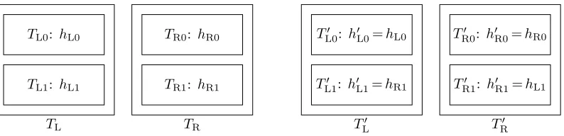
We describe a hashing scheme that uses two sets of tables. A left set including tables TL,TR, and a right set including tables TL0,TR0. Each table is also denoted as a “column”. Each table has two subtables, or “rows”. So overall there are four tables (columns), each containing two subtables (rows).
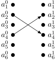
The tables. The construction uses two sets of tables,TL,TR andTL0,TR0. Each table is of size 2(1 +ε)n and is composed of two subtables of size (1 +ε)n(TL contains the subtables TL0,TL1, etc.). Each subtable is associated with a hash function that will be used by both parties. E.g., functionhL0 will be used for subtableTL0, etc. The tables and the hash functions are depicted in Figure 1.
The hash functions. The hash functions associated with the tables are defined as follows:
– The functions for the left two tables (columns)TL,TR, i.e.,hL0,hL1,hR0,hR1, are chosen at random. Each function maps items to the range [0,(1 +ε)n−1], which corresponds to the number of bins in each of TL0,TL1,TR0,TR1.
– The functions for the two right tables T0
L,TR0are defined as follows:
• The two functions of the upper subtables are equal to the functions of the upper subtables on the left. Namely,h0
L0=hL0 and h0R0=hR0.
• The two functions of the lower subtables are themirror imageof the functions of the lower subtables on the left. Namely,h0L1,h0R1are defined such thath0L1=hR1, andh0R1=hL1.
TL1: hL1
TL0: hL0
TL
TR1: hR1
TR0: hR0
TR
TL10 : h0L1=hR1
TL00 : h0L0=hL0
T0
L
TR10 : h0R1=hL1
TR00 : h0R0=hR0
T0
R
Fig. 1.The tablesTL,TRandTL0,T
0
R. The hash functions in the upper subtables ofT
0
L,T
0
Rare the same as inTL,TR,
and those in the lower subtables are in reverse order.
Bob’s insertion algorithm.Bob needs to insert each of his items to one subtable in each of the tables
TL,TR,TL0,TR0. He can do so by simply using Cuckoo hashing for each of these tables. For example, for the table TL and its subtablesTL0,TL1, Bob uses the functionshL0,hL1 to insert each input x to eitherTL0 or TL1. The same is applied toTR,TL0, andTR0. In addition, Bob keeps a small stash of size ω(1) for each of the four tables. Overall, based on known properties of Cuckoo hashing, we can claim that the construction guarantees the following property:
Claim.With all but negligible probability, it holds that for every inputxof Bob, and for each of the four tablesTL,TR,TL0,TR0, Bob insertsx to exactly one of the two subtables or to the stash.
Alice’s insertion algorithm.Alice’s operation is a little more complex and is described in Algorithm 1. Alice considers the two upper subtables on the left, TL0,TR0, as two subtables for standard Cuckoo hashing. Similarly, she considers the two lower subtables on the left,TL1,TR1, as two subtables for standard Cuckoo hashing. In other words, she considers the left top row and the left bottom row as standard Cuckoo hashing tables.
Algorithm 1 (Mirror Cuckoo hashing)
1. Alice uses Cuckoo hashing to insert each item x to one of the subtables TL0,TR0, using the hash
functionshL0,hR0.
2. Similarly, Alice uses Cuckoo hashing to insert each itemxto one of the subtablesTL1,TR1, using the
hash functionshL1,hR1.
3. At this point, Alice observes the result of the first two steps. For some inputsxit happened that they were mapped to the same “column” in both of these steps. Namely,xwas mapped to bothTL0 and
TL1, or to bothTR0 andTR1. These are the “good” items, since they were mapped to the same column,
as is required for all of Alice’s inputs.
4. The other inputs of Alice, the “bad” items, were mapped to one column in Step 1 and to the other column in Step 2. Alice applies the following procedure to these items:
(a) Each “bad” itemxis removed from both locations to which it was mapped in Steps 1 and 2. (b) xis now inserted in either ofTL00 ,T
0
R0 using the hash functionsh
0
L0:=hL0,h0R0:=hR0 with the
same mapping as in Step 1. (c) xis also inserted in either ofTL10 ,T
0
R1 using the hash functionsh
0
L1:=hR1,h0R1:=hL1with the
same mapping as in Step 2.
bottom row toTL1; or x is inserted in the top row toTR0 and in the bottom row toTR1. Therefore,
x is inserted in two subtables in the same column. (x is denoted as “good” since this is the outcome that we want.)
Let x0 be one of the other, “bad”, items. Thus,x0 is inserted in the top row to TL0 and in the bottom row to TR1, or vice versa. In this case, Alice removes x0 from the tables on the left and inserts it to the tablesTL0,TR0 on the right. Since the hash functions that are used inTL0,TR0 are equal to the functions used on the left side (where in the bottom row the functions are in reverse order), Alice does not need to run a Cuckoo hash insertion algorithm on the right side: Assume that x0
was stored in locations TL0[hL0(x0)] and TR1[hR1(x0)] on the left. Then Alice inserts it to locations
TL00 [h0L0(x0)] =TL00 [hL0(x0)] andTL10 [h0L1(x0)] =TL10 [hR1(x0)] on the right.
In other words, in a global view, one can see the algorithm as composed of the following steps: (1) First, all items are placed in the left tables. (2) Each subtable is divided in two copies, where one copy contains the good items and the other copy contains the bad items. (3) The subtable copies with the good items are kept on the left, whereas the copies with the bad items are moved to the right, where in the bottom row on the right we replace the order of the subtables.
This algorithm has two important properties: First, all items that were successfully inserted in the first step to the left tables will be placed in tables on either the left or the right hand sides. Moreover, each item will be placed in two subtables in the same column — the good items happened to initially be placed in this way in the left tables; whereas the bad items were in different columns on the left side but were moved to the same column on the right side. Hence, we can state the following claim:
Claim.With all but negligible probability, Alice inserts each of her inputs either to two locations in exactly one of TL,TR,TL0,TR0 and to no locations in other tables, or to a stash.
Tables size.The total size of the tables is 8(1 +ε)n.
simplicity, we omitted the stashes in Figure 1 and Algorithm 1.) Given the result of [KMW09], and our observation in §C about its applicability to non-constant stash sizes, it holds that a total stash of sizeω(1) elements suffices to successfully map all items, except with negligible probability. We note that the size of the stash can be arbitrarily close to constant, e.g., it can be set to be
O(log logn) or O(log∗n). Essentially, for any function f(n) ∈ω(n), the size of the stash can be
o(f(n)).
4.2 Circuit-based PSI from Mirror Cuckoo Hashing
Mirror Cuckoo hashing lets the parties map their inputs to tables of sizeO(n) and stashes of size
ω(1), with negligible failure probability. It is therefore straightforward to construct a PSI protocol based on this hashing scheme:
1. The parties agree on the parameters that define the size of the tables and the stash for mirror Cuckoo hashing. They also agree on the hash functions that will be used in each table.
2. Each party maps its items to the tables using the hash functions that were agreed upon. 3. The parties evaluate a circuit that performs the following operations:
(a) For each bin in the tables, the circuit compares the item that Alice mapped to the bin to the item that Bob mapped to the same bin.
(b) Each item that Bob mapped to his stashes is compared with all items of Alice. Similarly, each item that Alice mapped to her stashes is compared with all items of Bob.
The properties of mirror Cuckoo hashing ensure: (1) If an itemx is in the intersection, then there is exactly one comparison in whichx is input by both Alice and Bob. (2) The number of comparisons in Step 3 isω(n).
5 A Concretely Efficient Construction through 2D Cuckoo Hashing
Two-dimensional Cuckoo hashing (a.k.a. 2D Cuckoo hashing) is a new construction with the following properties:
– It uses overall O(n) memory (specifically, 8(1 +ε)n in our construction, where we setε= 0.2 in our experiments).
– Both, Alice and Bob, map each of their items to O(1) memory locations (specifically, to two or four memory locations in our construction).
– If xappears in the input of both parties, then there is exactly one location to which both Alice and Bob map x.
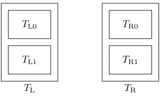
The construction uses two tables, TL,TR, located on the left and the right side, respectively. Each of these tables is of size 4(1 +ε)n and is composed of two smaller subtables:TL is composed of the two smaller subtables TL0,TL1, whileTR is composed of the two smaller tables TR0,TR1. The hash functions hL0,hL1,hR0,hR1 are used to map items toTL0,TL1,TR0,TR1, respectively. The tables are depicted in Figure 2.
Hashing is performed in the following way:
– Alice maps each of her items to all subtables on one of the two sides. Namely, each item x
of Alice is either mapped to both bins TL0[hL0(x)] and TL1[hL1(x)] on the left side, or to bins
TL1
TL0
TL
TR1
TR0
TR
Fig. 2.The tablesTLandTR, consisting of TL0,TL1andTR0,TR1, respectively.
– Bob maps each of his items to one subtable on each side. This is done using standard Cuckoo hashing. Namely, each inputxof Bob is mapped to one of the locationsTL0[hL0(x)] orTL1[hL1(x)] on the left side, as well as mapped to one of the locations TR0[hR0(x)] or TR1[hR1(x)] on the right side. In other words, BOB maps each item to one subtable on BOTH sides.
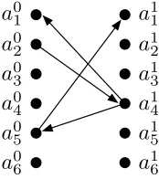
The possible options for hashing an item xby both parties are depicted in Figure 3. It is straightfor-ward to see that if both parties have the same itemx, there is exactly one table out ofTL0,TL1,TR0,TR1 that is used by both Alice and Bob to storex.
Alice Bob
Fig. 3.The possible combinations of locations to which Alice and Bob map their inputs.
We next describe a construction of 2D Cuckoo hashing, followed by a variant based on a heuristic optimization that stores two items in each table entry. The asymptotic behavior of the basic construction is analyzed in §A. In §6.1 we describe simulations for setting the parameters of the heuristic construction in order to reduce the hashing failure probability to below 2−40.
5.1 Iterative 2D Cuckoo Hashing
Algorithm 2 (Iterative 2D Cuckoo hashing)
1. Alice maps all of her items to table TL, using simple hashing. That is, each item xis inserted in
locationshL0(x), hL1(x). Obviously, there will be entries inTLthat will have more than a single item
mapped to them.
DenoteTLas the active table.
2. For each entry in the active table with more than one item in it: remove all items – except for the item that was mapped to this entry most recently – and move them to the “relocation pool”. For each of the removed items, remove the item also from its other appearance in the active table. (At the end of this step, all entries in the active table have at most one entry. However, there might be items in the relocation pool.)
3. If the relocation pool is empty, then stop (found a successful mapping). 4. Change the designation of the active table to point to the other table.
5. Move each itemxfrom the relocation pool to locationsh0(x), h1(x) in the active table. (For example,
ifTR is the active table, movextohR0(x), hR1(x).)
6. Go to Step 2.
is conceptually simpler to understand.) The parties associate two hash functions with each table, namely hL0,hL1 forTL, and hR0,hR1 forTR.
As in the mirror Cuckoo hashing construction described in §4.1, Bob uses Cuckoo hashing to insert each of his items into one location in each of the tables.
Alice inserts each item x either into the two locationshL0(x) and hL1(x) in TL, or into the two locations hR0(x) and hR1(x) in TR. This is achieved by Alice running a modified Cuckoo insertion algorithm that maps an item to two locations in one table, “kicks out” any item that is currently present in these locations and also removes the other occurrence of this item from the table, and then tries to insert this item into its two locations in the other table, and so on.
This is a new variant of Cuckoo hashing, where inserting an item into a table might result in four elements that need to be stored in the other table: storing x inhL0(x), hL1(x) might remove two items,y0, y1, one from each location. These items are also removed from their other occurrences inTL. They must now be stored in locations hR0(y0), hR1(y0), hR0(y1), hR1(y1) in TR.
It is not initially clear whether such a mapping is possible (with high probability, given random choices of the hash functions). We analyze the construction in §A and show that it only fails with probabilityO(1/n). We ran extensive simulations, showing that the algorithm (when using a stash and a certain choice of parameters) fails with very small probability, smaller than 2−40.
The insertion algorithm of Alice is described in Algorithm 2. The choice made in Step 2 of the algorithm, to first remove the oldest items that were mapped to the entry, is motivated by the intuition that it is more likely that the locations to which these items are mapped in the other table are free.
Storing two items per bin. It is known that the space utilization of Cuckoo hashing can be improved by storing more than one item per bin (cf. [Pan05, DW07] or the review of multiple choice hashing in [Wie16]). We take a similar approach and use two tables of size 2(1 +ε)nwhere each entry can storetwoitems. (These tables have half as many entries as before, but each entry can store two items rather than one. The total size of the tables is therefore unchanged.) The change to the insertion algorithm is minimal and affects only Step 2. The new algorithm is defined in Algorithm 3.
Algorithm 3 (Iterative 2D Cuckoo hashing with bins of size 2)
The algorithm is identical to Algorithm 2, except for the following change in Step 2:
2. For each entry in the active table with more thantwoitems in it: remove all items – except for thetwo
items that were mapped to this entry most recently – and move them to the “relocation pool”. For each of the removed items, remove the item also from its other appearance in the active table.
it achieves a lower probability of hashing failure, namely of the need to use the stash, and requires less iterations to finish.
5.2 Circuit-based PSI from 2D Cuckoo Hashing
This section describes how 2D Cuckoo hashing can be used for computing PSI. In addition, we describe two optimizations which substantially improve the efficiency of the protocol. The first optimization has the parties use permutation-based hashing [ANS10] (as was done in [PSSZ15]) in order to reduce the size of the items that are stored in each bin, and hence reduce the number of gates in the circuit. The second optimization is based on having each party use a single stash instead of using a separate stash for each Cuckoo hashing instance.
The PSI protocol is pretty straightforward given 2D Cuckoo hashing:
First, the parties agree on the hash functions to be used in each table. (These functions must be chosen at random, independently of the inputs, in order not to disclose any information about the inputs. Therefore, a participant cannot change the hash functions if some items cannot be mapped, and thus we seek parameter values that make the hashing failure probability negligible, e.g., smaller than 2−40.)
Then, each party maps its items to bins using 2D Cuckoo hashing and the chosen hash functions. The important property is that if Alice and Bob have the same input item then there exists exactly one bin into which both parties map this item (or, alternatively, at least one of them places this item in a stash). Empty bins are padded with dummy elements. This ensures that no information is leaked by how empty the tables and stashes are.
Afterwards, the parties construct a circuit that compares, for each bin, the items that both parties stored in it. In addition, this circuit compares each item that Alice mapped to the stash with all of Bob’s items, and vice versa. Since the number of bins is O(n), the number of items in each bin isO(1), and the number of items in the stash is ω(1), the total size of this circuit isω(n). The parties can define another circuit that takes the output of this circuit and computes a desired function of it, e.g., the number of items in the intersection.
Finally, the parties run a generic MPC protocol that securely evaluates this circuit (cf.§6.3 for a concrete implementation and benchmarks).
element x to bin xL⊕f(xR) and the value stored in the bin isxR. The important property is that the stored value has a reduced bitlength of only |x| −logβ, yet there are no collisions (since if x, y
are mapped to the same bin and store the same value, then xR=yR andxL⊕f(xR) =yL⊕f(yR) and therefore x=y).
In the general case, whereβ is not a power of two, the output ofh is reduced moduloβ and a stored extra bit indicates if the output was reduced or not.
For Cuckoo hashing the protocol uses two hash functions to map the elements to the bins in one table. To avoid collisions among the two hash functions, a stored extra bit indicates which hash function was used.
Using a Combined Stash. Recall that Alice uses 2D Cuckoo hashing, for which we show experimentally in §6.1 that no stash is needed. Bob, on the other hand, uses two invocations of standard Cuckoo hashing, and therefore when he does not succeed in mapping an item to a table, he must store it in a stash and compare it with all items of Alice. In this case, the parties cannot encode their items using permutation-based hashing, and therefore these comparisons must be of the full-length original values and not of the shorter values computed using permutation-based hashing as described before. Therefore, the size of the circuits that handle the stash values have a considerable effect on the total overhead of the protocol.
We observe that, instead of keeping several stashes, Bob can collect all the values that he did not manage to map to any of the tables in acombinedstash. Suppose that he maps items toctables and that we have an upper boundswhich holds w.h.p. on the size of each stash. A naive approach would use cstashes of that size, resulting in a total stash size ofc·s. A better approach would be to use a single stash for all these items, since it is very unlikely that all stashes will be of maximal size, and therefore we can show that with the same probability, the sizes0of the combined stash is much smaller
thanc·s. To do so, we determine the upper bounds for the combined stash forc= 2: The probability of having a combined stash of size s0 isPs0
i=0P(i)·P(s
0−i), where P(i) denotes the probability of
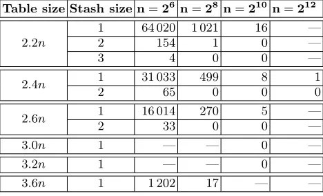
having a single stash of sizei. The value ofP(i) isO(n−i)−O(n−(i+1))≈O(n−i) [KMW09]. We can estimate the exact values of these probabilities based on the experiments conducted by [PSSZ15]: they performed 230 Cuckoo hashing experiments for eachn∈ {211,212,213,214} and counted the required stash sizes. Using linear regression, we extrapolated the results for larger sets of 216and 220 elements. Table 1 shows the required stash sizes when binding the probability to be below 2−40: it turns out that for 212 and 216 elements the combined stash should include only one more element compared to the upper bound for a single stash, whereas for 220even the same stash size is sufficient. All in all, when comparing to the naive solution with two separate stashes, the combined stash size is reduced by almost a factor of 2x.
Table 1.Stash sizes required for binding the error probability to be below 2−40 when insertingn∈ {212,216,220} elements into 2.4nbins using Cuckoo hashing.
Number of elements n 212 216 220
Single stash sizes(from [PSSZ15, Table 4]) 6 4 3 Stash size for two separate stashess0= 2s 12 8 6
5.3 Extension to a Larger Number of Parties
Computing PSI between the inputs of more than two parties has received relatively little interest. (The challenge is to compute the intersection of the inputs of all parties, without disclosing information about the intersection of the inputs of any subset of the parties.) Specific protocols for this task were given, e.g., in [FNP04, HV17, KMP+17]. We note that our 2D Cuckoo hashing can be generalized tom dimensions in order to obtain a circuit-based protocol for computing the intersection of the inputs of mparties. The caveat is that the number of tables grows to 2m and therefore the solution is only relevant for a small number of parties.
We describe the case of three parties: The hashing will be to a set of eight tablesTx,y,z, where x, y, z∈ {0,1}. Any input item of P1 is mapped to either all tablesT0,0,0, T0,0,1, T0,1,0, T0,1,1, or to all tablesT1,0,0, T1,0,1, T1,1,0, T1,1,1. Namely, the indexxis set to either 0 or 1, and the input item is mapped to all tables with that value of x. Every input ofP2 is mapped either to all tables whosey index is 0, or to all tables where y= 1. Every input of P3 is mapped either to all tables whose z index is 0, or to all tables wherez= 1.
It is easy to see that regardless of the choices of the values ofx, y, z, the sets of tables to which all parties map an item intersect in exactly one table. Therefore, the parties can evaluate a simple circuit that checks every bin for equality of the values that were mapped to it by the three parties. It is guaranteed that if the same value is in the input sets of all parties, then there is exactly one bin to which this value is mapped by all three parties. If some items are mapped to a stash by one of the parties, they must be compared with all items of the other parties, but the overhead of this comparison is ω(n) if the stash is of sizeω(1).
The remaining issue is the required size of the tables. In §A.4 we show that inserting an item into one of two (big) tables, such that the item is mapped to k locations in that table, requires tables of size greater thank2(1 +ε)n. When computing PSI between three parties using the method described above, we have eight (small) tables, where each party must insert its items to four tables in one plane or to four tables in the other plane. Each such set of four small tables corresponds to a big table in the analysis of§A.4 and is therefore of size 16(1 +ε)n. The total size of the tables is therefore 32(1 +ε)n.
5.4 No Extension to Security against Malicious Adversaries
We currently do not see how to extend our hashing-based protocols to achieve security against malicious adversaries. As pointed out by [RR17b], it is inherently hard to extend protocols based on Cuckoo hashing to obtain security against malicious adversaries. The reason is that the placement of items depends on the exact composition of the input set, and therefore a malicious party might learn the placement used by the other party.
6 Evaluation
This section describes extensive experiments that set the parameters for the hashing schemes, the resulting circuit sizes, and the results of experiments evaluating PSI using these circuits.
6.1 Simulations for Setting the Parameters of 2D Cuckoo Hashing
We experimented with the iterative 2D Cuckoo hashing scheme described in §5.1, set concrete sizes for the tables, and examined the failure probabilities of hashing to the tables.
Our implementation is written in C and available online athttp://encrypto.de/code/2DCu ckooHashing. It repeatedly inserts a set of random elements into two tables using random hash functions. The insertion algorithm is very simple: All elements are first inserted into the two locations to which they are mapped (by the hash functions) in the first table. Obviously, many table entries will contain multiple items. Afterwards, the implementation iteratively moves items between the tables, in order to reduce the maximum bin occupancy below a certain threshold (cf. Algorithm 2 and Algorithm 3 in§5.1).
Run-time. We report in§6.3 the results of experiments analyzing the run-time of the 2D Cuckoo hashing insertion algorithm. Overall, the insertion time (a few milliseconds) is negligible compared to the run-time of the entire PSI protocol.
Hashing to bins of size 1. First, we checked if it is possible to use a maximum bin occupation of 1. For this, we set the sizes of each of the two tables to be 4.8n(corresponding to the threshold size of 4(1 +ε)nin the analysis in §A, as well as twice the recommended size for Cuckoo hashing, since all elements are inserted twice). We ran the experiment 100 000 times with input size n= 212 and bitlength 32. For all except 828 executions it was possible to reduce the maximum bin occupation to 1 after at least 7 and at most 129 iterations of the insertion algorithm. On average, 20 iterations of the insertion algorithm were necessary to achieve the desired result. In said 828 cases there remained at least one bin with more than one item even after 500 iterations of the insertion algorithm. This implies that iterative 2D Cuckoo hashing works in principle, but, as standard Cuckoo hashing, requires a stash for storing the elements of overfull bins.
Hashing to bins of size 2. For PSI protocols it would be desirable to avoid having an additional stash on Alice’s side. In standard Cuckoo hashing it is possible to achieve better memory utilization and less usage of the stash by using fewer bins, where each bin can store two items [Wie16]. Therefore, we changed the parameters as follows: the table size is halved and reduced to 2.4n, but each bin is allowed to contain two elements. This way, while consuming the same amount of memory as before, we try to achieve better utilization. We followed the paradigm that was described in§3.2 for the experimental analysis of the failure probability. Namely, we ran massive sets of experiments to measure the number of failures for several values ofnand several table sizes, and given this data we (1) found confidence intervals for the failure probability for specific values of the parameters, and (2) found how the failure probability behaves as a function ofn.
Our first experiment ran 240 tests within ∼ 2 million core hours on the Lichtenberg6 high performance computer of the TU Darmstadt for input size n= 212. We chose input size 212 (instead
6
of larger sizes like 216 or 220) since running experiments with larger values ofnwould have taken even more time and would have simply been impractical. It turned out that the insertion algorithm was successful in reducing the maximum bin size to 2 (after at most 18 iterations) in all but one test.
Given this data, we calculated the confidence interval of the failure probabilityp. The probability of observing one failure in N experiments isN ·p·(1−p)N−1, where in our experimentsN = 240. We checked the values ofp for which the probability of this observation is greater than 0.001 and concluded that with 99.9% confidence, the failure probability for iterative 2D Cuckoo hashing with set size n = 212 and table size 2.4n lies within
2−50,2−37
. (Namely, there is at most a 0.001 probability that we would have seen one failure in 240 runs ifp was greater than 2−37 or smaller than 2−50.)
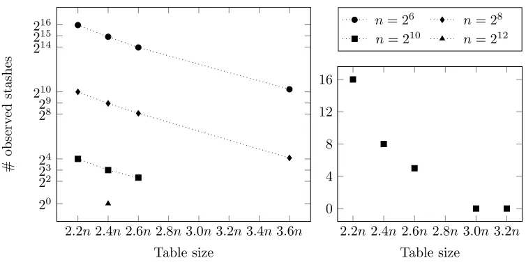
Measuring the dependence on the parameters. To get a better understanding on how the failure probability behaves for different input and table sizes, we performed a set of experiments that required another ∼ 3.5 million core hours. Concretely, we ran 240 tests for each set size
n ∈ {26,28,210} and each table size in the range 2.2n, 2.4n, and 2.6n. We also tested the table size 3.6n for n ∈ {26,28} as well as table sizes 3.0n and 3.2n for n = 210. The results for all experiments are given in Table 2 and are depicted in Figure 4.
The results demonstrate that, w.r.t. the dependence on n, for set sizesn∈ {26,28,210} it can be observed that increasing the set size by factor 4x reduces the failure probability by factor 64x. (For larger set sizes, the number of failures is too small to be meaningful.) These experiments also
demonstrate that the dependence of the failure probability onnis O(n−3). An intuitive theoretical explanation why the probability behaves this way is given in §B. As for the dependence on the table size, the failure probability decreases by a factor of 2x when increasing the table size in steps of 0.2n
within the tested range 2.2n to 3.6n.
From these results (a failure probability of at most 2−37 forn= 212with table size 2.4nand a dependence ofO(n−3) of the failure probability on n) we conclude that the failure probability for
n≥213 and table size 2.4n is at most 2−40.
In total we spent about 5.5 million core hours on our experiments on the Lichtenberg high performance computer of the TU Darmstadt.
Table 2.Number of observed stashes for different table sizes and set sizesnwhen performing 240tests of iterative 2D
Cuckoo hashing.
Table size Stash size n=26 n=28 n=210 n=212
2.2n
1 64 020 1 021 16 —
2 154 1 0 —
3 4 0 0 —
2.4n 1 31 033 499 8 1
2 65 0 0 0
2.6n 1 16 014 270 5 —
2 33 0 0 —
3.0n 1 — — 0 —
3.2n 1 — — 0 —
2.2n2.4n2.6n2.8n3.0n3.2n3.4n3.6n
20
22
23
24
28
29
210
214
215
216
Table size
#
observ
ed
stashes
n= 26 n= 28
n= 210 n= 212
2.2n2.4n2.6n2.8n3.0n3.2n
0 4 8 12 16
Table size
Fig. 4.Number of observed stashes for different table and set sizes when performing 240 tests of iterative 2D Cuckoo
hashing.
6.2 Circuit Complexities
We compare the complexities of the different circuit-based PSI constructions for two sets, each with nelements that have bitlengthσ. We consider two possible bitlengths:
1. Fixed bitlength: Here, the elements have fixed bitlengthσ = 32 bits (e.g., for IPv4 addresses). 2. Arbitrary bitlength:Here, the elements have arbitrary bitlength and are hashed to values of
length σ = 40 + 2 log2(n)−1 bits, with a collision probability that is bounded by 2−40. (See Appendix A of the full version of [PSZ14] for an analysis.) Therefore, we set the bitlength to
σ = 40 + 2 log2(n)−1 bits.
For all protocols we report the circuit size where we count only the number of AND gates, since many secure computation protocols provide free computation of XOR gates. We compute the size of the circuits up to the step where single-bit wires indicate if a match was found for the respective element. We note that for many circuits computing functions of the intersection, this part of the circuit consumes the bulk of the total size. For example, computing the Hamming weight of these bits is equal to computing the cardinality of the intersection (PSI-CA). The size-optimal Hamming weight circuit of [BP06] has size x−wH(x) and depth log2x, where x is the number of inputs and wH(·) is the Hamming weight. The size of the Hamming weight circuit is negligible compared to the rest of the circuit. As another example, if the cardinality is compared with a threshold (yielding a PSI-CAT protocol), this only adds 3 log2n AND gates and depth log2log2n using the
depth-optimized construction described in [SZ13], which is also negligible.
single bit that indicates if a match was found for the respective element or not; this removes n
multiplexers ofσ-bit values from the COMPARE phase, i.e., σnAND gates. Hence, the total size is 2σnlog2(n) + 2σn−n−σ+ 2 AND gates.
The size of the Circuit-Phasing circuit. The Circuit-Phasing circuit [PSSZ15] has 2.4nm(σ − log2(2.4n) + 1) +sn(σ−1) AND gates where m is the maximum occupancy of a bin for simple hashing and sis the size of the stash.
The size of our mirror Cuckoo hashing construction of §4.2. In this protocol, Bob uses a total of four Cuckoo hash tables, so he needs four stashes. Alice uses Cuckoo hashing for the first set of tables, and then she essentially applies the same Cuckoo hashing in reverse order for the second set of tables, so she needs only two stashes. The total number of stashes is hence 6. The protocol compares 4 times the shortened representations (using permutation-based hashing) for Cuckoo tables with 2.4nbins and 6 stashes ofselements each with nelements using the full representation ofσ bits. Hence, the total complexity is 4·2.4n(σ−log2(2.4n) + 1) + 3s0n(σ−1), wheres0 ≤2sis
the size of the combined stash. (The concept of the combined stash, cf. §5.2, can also be applied to the mirror Cuckoo hashing construction).
The size of our iterative 2D Cuckoo hashing construction of§5.2. Each of the following operations is performed twice for the left and right side: (1) For each of the 2.4nbins the shortened representation (cf.§5.2) of the single item in Bob’s bin is compared with the two elements in the corresponding bin of Alice. (2) Bob has a stash of sizes0. Each item in the stash is compared to all of Alice’s items (using the
full bitlength representation). Hence, the overall complexity is 4·2.4n(σ−log2(2.4n) + 1) +s0n(σ−1) AND gates, where s0 is the size of the combined stash. By comparing this formula with the one for the mirror construction above we directly see that the iterative construction is always better as it requires only one combined stash.
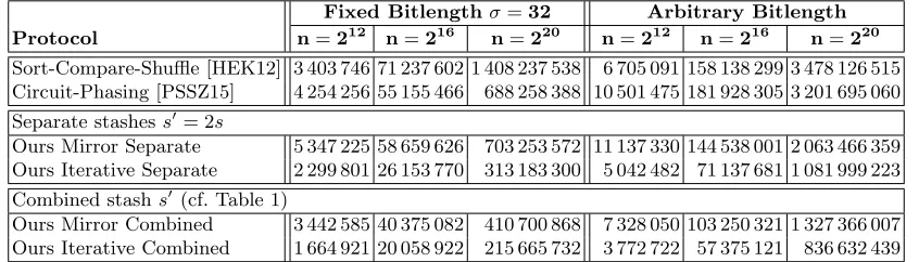
Concrete Circuit Sizes. The Sort-Compare-Shuffle construction [HEK12] has a circuit of size
O(σnlogn). The Circuit-Phasing construction [PSSZ15] has circuit sizeO(σnlogn/log logn), while the asymptotic construction we present in this paper has a size ofω(σn) and the iterative 2D Cuckoo hashing construction has an even smaller size.
For a comparison of the concrete circuit sizes, we use the parameters from the analysis in [PSSZ15]: For n= 212 elements the maximum bin size for simple hashing is m= 18, for n= 216 we set m= 19, and for n= 220 we setm= 20. We set the stash size sand the combined stash sizes0
according to Table 1 (on page 17).
On the left side of Table 3 we compare the concrete circuit sizes for fixed bitlength σ= 32 bit. Our best protocol (“Ours Iterative Combined”) improves over the best previous protocol by factor 2.0x forn= 212 (over [HEK12]), by factor 2.7x forn= 216 (over [PSSZ15]), and by factor 3.2x for
n= 220 (over [PSSZ15]).
On the right side of Table 3 we compare the concrete circuit sizes for arbitrary bitlength σ. Our best protocol (Ours Iterative Combined) improves over the best previous protocol by factor 1.8x for
n= 212 (over [HEK12]), by factor 2.8x for n= 216 (over [HEK12]), and by factor 3.8x for n= 220 (over [PSSZ15]).
constructions, and, due to our better asymptotic size, the savings become greater as nincreases. (The Sort-Compare-Shuffle construction of [HEK12] performs better than the Phasing construction
of [PSSZ15] for smaller values of n, but for larger values it is the opposite. This is expected, as the asymptotic sizes areO(σnlogn) and O(σnlogn/log logn), respectively.)
Table 3.Concrete circuit sizes in #ANDs for PSI variants onnelements of fixed bitlengthσ= 32 (left) and arbitrary bitlength hashed toσ= 40 + 2 log2(n)−1 bits (right).
Fixed Bitlengthσ=32 Arbitrary Bitlength Protocol n=212 n=216 n=220 n=212 n=216 n=220
Sort-Compare-Shuffle [HEK12] 3 403 746 71 237 602 1 408 237 538 6 705 091 158 138 299 3 478 126 515 Circuit-Phasing [PSSZ15] 4 254 256 55 155 466 688 258 388 10 501 475 181 928 305 3 201 695 060
Separate stashess0= 2s
Ours Mirror Separate 5 347 225 58 659 626 703 253 572 11 137 330 144 538 001 2 063 466 359 Ours Iterative Separate 2 299 801 26 153 770 313 183 300 5 042 482 71 137 681 1 081 999 223
Combined stashs0(cf. Table 1)
Ours Mirror Combined 3 442 585 40 375 082 410 700 868 7 328 050 103 250 321 1 327 366 007 Ours Iterative Combined 1 664 921 20 058 922 215 665 732 3 772 722 57 375 121 836 632 439
Circuit Depths. For some protocols, the circuit depth is a relevant metric (e.g., for the GMW protocol the depth determines the round complexity of the online phase). Our constructions have the same depth as the Circuit-Phasing protocol of [PSSZ15], i.e., log2σ. This is much more efficient than the depth of the Sort-Compare-Shuffle circuit of [HEK12] which is O(logσ·logn) when using depth-optimized comparison circuits.
Further Optimizations. So far, we computed the comparisons with a Boolean circuit consisting of 2-input gates: For elements of bitlength`, the circuit XORs the elements and afterwards computes a tree of `−1 non-XOR gates s.t. the final output is 1 if the elements are equal or 0 otherwise. This circuit allows to use an arbitrary secure computation protocol based on Boolean gates, e.g., Yao or GMW. However, the construction of evaluating 2-input gates in GMW using 1-out-of-4 OTs described in [Gol04, Sect. 7.3.3] can easily be generalized to evaluating d-input gates with 1-out-of-2dOTs which can be instantiated very efficiently with the 1-out-of-N OT extension protocol of [KK13].7 Further optimizations and an implementation are described in [DKS+17] who call these
d-input gates lookup tables (LUTs). Their best LUT has 7 inputs and requires only 372 bits of total communication (cf. [DKS+17, Tab. IV]). For computing equality, 6 of the non-XOR gates in the tree can be combined into one 7-input LUT. This improves communication of the Circuit-Phasing protocol of [PSSZ15] and our protocols by factor 6·256/372 = 4.1x.
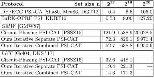
6.3 Performance
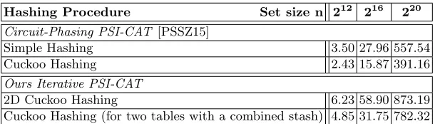
We empirically compare the performance of our iterative 2D Cuckoo hashing PSI-CAT protocol with a combined stash described in §5.2 with the Circuit-Phasing PSI-CAT protocol of [PSSZ15]. As
7