Overview of Modelling and Control Strategies for
Wind Turbines and Hydroelectric Systems:
Comparisons and Contrasts
†
Silvio Simani∗, Stefano Alvisi, Mauro Venturini
Department of Engineering, University of Ferrara, Via Saragat 1E – 44122, Ferrara (FE), Italy * Email: [email protected], tel/fax: +39 0532 97 4844.
Abstract: Increasingly, there is a focus on utilising renewable energy resources in a bid to fulfil increasing energy requirements and mitigate the climate change impacts of fossil fuels. While most renewable resources are free, the technology used to usefully convert such resources is not and there is an increasing focus on improving the conversion economy and efficiency. To this end, advanced control technologies can have a significant impact and is already a relatively mature technology for wind turbines. Though hydroelectric plants can use simple regulation systems, significant benefits have been shown to accrue from the appropriate use of the same control methods designed for wind turbine plants. This represents the key point of the paper. In fact, to date, the application communities connected with wind and hydraulic energies have had little communication, resulting in little cross fertilisation of control ideas and experience, particularly from the more mature wind area to hydrodynamic systems. Therefore, this paper examines the models and the application of control technology across both domains, both from a comparative and contrasting point of view, with the aim of identifying commonalities in models and control objectives, as well as potential solutions. Key comparative reference points include the articulation of the exployed models, specification of control objectives, development of high–fidelity simulators, and development of solution concepts. Not least, in terms of realistic system requirements are the set of physical and constraints under which such renewable energy systems must operate, and the need to provide reliable and robust control solutions, which respect the often remote and relatively inaccessible location of many onshore and offshore deployments.
Keywords: wind turbines; hydroelectric systems; nonlinear modelling; model–based control; data–driven approach; advanced control; robustness and reliability
1. Introduction
With the continuing decrease in the stock of global fossil fuels, issues of security of supply, and pressure to honour greenhouse gas emission limits (e.g., the Kyoto protocol), much attention has turned to renewable energy sources to fulfil future increasing energy needs. Wind energy, now a mature technology, has had considerable proliferation, with other sources, such as biomass, solar, and hydraulic, enjoying somewhat less deployment. Hydraulic power provides previously untapped energy potential, and hydroelectric systems can show some variability properties (a perennial issue with many renewable, especially wind), especially when combined with wind energy.
One common misconception, in effective renewable energy converter design, is that converters must be optimally efficient. However, since the resource itself (wind and hydraulic power) is free, the main objective is to minimise the converted cost of the renewable energyi.e.the cost per kWh, taking into account the lifetime costs (capital, operational and commissioning/decommissioning costs) as well as energy receipts (value of energy sold). Nevertheless, for a given capital cost, maximising the energy receipts (assuming relative insensitivity of operational costs) is an important economic objective and control system technology has an important role to play in this regard. In an ideal world, one should consider the design of a complete system from the top down. However, convention has it that physical systems are usually designed by the discipline–specific experts and the control problem
is then addressed in a subsequent step by control engineers, working in collaboration with the discipline–specific experts. Such an approach, though prevalent in the bulk of industrial applications of control, is non–optimal, even if there are some notable exceptions.
Some preliminary studies do suggest a strong interaction between the fundamental design of renewable energy conversion machines and the algorithms and systems used to control them [1,2]. In any case, given the relatively low cost of control systems technology (sensors, actuators, computer, software) compared to the cost of the renewable energy converters [3]), it will be assumed in this paper that the focus is on increasing the energy conversion capacity of a given wind turbine or hydroelectric system device. However, this relatively simple implementation modality masks both the capability of control systems and the high level of engineering underpinning the development of a suitable control algorithm. For example, many high–performance model–based control design methods require an accurate mathematical model of the system to be controlled and a significant number of man–hours can be absorbed in modelling. Nevertheless, there is usually a good case to be made for the incorporation of control technology to improve the performance (both technical and economic), reliability and safety of a system [4]. By taking into account commonalities and contrasts in particular for wind turbines and hydroelectric systems, this work will consider the role that modelling and control engineering can play in making energy conversion systems more competitive and effective.
There are a number of economic issues associated with the introduction of control systems for renewable energy devices which need to be considered. One important factor is that many wind turbine and hydroelectric devices are situated in relatively remote and/or inaccessible areas, with consequent implications for maintenance. As a result, the implemented control systems should be reliable and there is a need for fault–tolerant control [5]. In addition, any increases in duty cycle, velocities or forces associated with energy converter components need to be considered and these may impact operational cost via additional maintenance requirements.
Both wind turbines and hydroelectric systems exhibit nonlinear behaviour and are required to operate over a wide range of excitations. These energy conversion systems also have particular physical constraints (displacements, velocities, accelerations and forces) which must be strictly observed if such systems are to operate effectively and have economically attractive useful operational lifetimes. The motivation for this paper comes from a real need to have an overview on the modelling and control challenges for wind turbines and hydroelectric systems, which present common and different requirements related to renewable source power conversion efficiency into electric energy. In general, in the fields considered in this paper, power conversion is converting renewable sources to electric energy, regulating also the voltage and frequency. Therefore, a power converter is an electro–mechanical device for converting wind/hydraulic energy to electrical energy. The power converter includes an electrical machinery that is used to convert and control both frequency and voltage.
With this view, the work will focus on commonalities and contrasts for wind and hydraulic energy systems. Wind turbine systems seem relatively mature from the modelling point of view, whilst hydraulic energy devices present unique, interesting and challenging aspects. Therefore, the final aim is to see what modelling and control aspects might be common with a view to utilising some ideas, born in one domain, within the other. These issues have begun to stimulate research and development in the wider control community in each domain, and the main results will be summarised in this work. In particular, a proper mathematical description of these energy conversion systems should be able to capture the complete behaviour of the process under monitoring, thus providing an important impact on the control design itself.
Therefore, the analysis of the commonalities and the contrasts between these two fields will be performed according the following items, which describe also the structure of the paper:
• Requirements of the generic control problem: unique aspects to wind turbine and hydroelectric systems;
• Control strategy development: objectives and available tools for wind turbines and hydroelectric systems;
• Conclusions: are these two domains really comparable? On what basis – modelling and/or control, and/or the intermittent resource that drive them? Are there some fundamental issues, from a control perspective?
2. Overview of Energy Conversion Models and Baseline Controllers
This section summarises the models and the traditional control schemes commonly used for the description of the wind turbines, recalled in Section2.1, and the hydroelectric system devices, addressed in Section2.2.
2.1. Wind Turbine Systems
Wind energy can be considered as a fast–developing multidisciplinary field consisting of several branches of engineering sciences. The National Renewable Energy Laboratory (NREL) estimated a growth rate of the wind energy installed capacity of about 30% from 2001 to 2006, [6], and even with a faster rate up to 2016 [7]. From 2009, 83 countries around the world are exploiting wind energy on a commercial basis, as wind power is considered as a renewable, sustainable and green solution for energy harvesting. Note however that, even if the U.S. now achieves less than 2% of its required electrical energy from wind, the most recent NREL’s report states that the U.S. will increase it up to 30% by the year 2030 [7]. Note also that, even if the fast growth of the wind turbine installed capacity of wind turbines in recent years, multidisciplinary engineering and science challenges still exist [8]. Moreover, wind turbine installations must guarantee both power capture and economical advantages, thus motivating the wind turbine dramatic growth [7].
Industrial wind turbines have large rotors and flexible load–carrying structures that operate in uncertain and noisy environments, thus motivating challenging cases for advanced control solutions, which this paper will consider for comparison purposes. Advanced controllers can be able to achieve the required goal of decreasing the wind energy cost by increasing the capture efficacy; at the same time they should reduce the structural loads, thus increasing the lifetimes of the components and turbine structures [9]. This paper aims also at sketching the main challenges and the most recent research topics in this area, when considering both wind turbines and hydroelectric systems. Although wind turbines can be developed in both vertical–axis and horizontal–axis configurations, this paper is focussed on horizontal–axis wind turbines, which represent the most common solutions today in large–scale installations.
The three–bladed horizontal axis turbine considered in this paper works according to the principle that the wind is acting on the blades, and thereby moving the rotor shaft. In order to up–scale the rotational speed to the needed one at the generator, a gear box is introduced. A more accurate description of the benchmark can be founde.g.in [10,11]. A schematic diagram of the wind turbine system and its main variables is depicted in Figure1.
The rotational speed, and consequently the generated power, is regulated by means of the two control inputs: the converter torqueτg(t)and the pitch angle β(t)of the turbine blades. From the
wind turbine system, a number of measurements can be acquired: ωr(t)is the rotor speed,ωg(t)is
the generator speed,τg(t)the torque of the generator controlled by the converter, which is provided
with the torque reference,τr(t). The estimated aerodynamic torque is defined asτaero(t). This estimate
Figure 1.Wind turbine general scheme and its main variables.
can be considered disturbances for control design. Moreover, the aerodynamic torque depends on another uncertain term,Cp, representing the power coefficient, as shown by Eq. (1):
τaero(t) =
ρA Cp(β(t),λ(t)) v3(t)
2ωr(t) (1)
whereρis the density of the air,Ais the area covered by the turbine blades in its rotation, whilstλ(t)
is the tip–speed ratio of the blade, defined as:
λ(t) = ωr(t)R
v(t) (2)
with R the rotor radius. Cp represents the power coefficient, which the wind turbine benchmark
implements by means of a two–dimensional map (look–up table) [10]. Equation (1) is used to estimate
τaero(t)based on an assumed estimatedv(t), and the signalsβ(t)andωr(t). Due to the uncertainty
of the wind speedv(t), the termτaero(t)is considered affected by an unknown error. Moreover, the
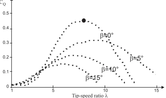
nonlinearity represented by Eqs. (1) and (2) is sketched in Figure2for different values ofλ(t)(i.e. v(t)) andβ(t).
CQ
Tip-speed ratiol
b=0°
b=5° b=10°
b=15°
0.5
0.4
0.3
0.2
0.1
0
1 5 10 15
Figure 2.Example power curves.
If a simple one–body model is used to represent the drive train [11], the complete continuous–time description of the wind turbine model has the form of Eq. (3):
˙
x(t) = fc(x(t),u(t))
y(t) = x(t)
whereu(t) = [τr(t)β(t)]Tandy(t) =x(t) =ωr(t)τg(t)Tare the control inputs and the monitored
output measurements, respectively. fc(·)represents the continuous–time nonlinear function that will
be used for acquiring the Nsampled data u(k)and y(k), with k = 1, 2, . . .N. Finally, the model parameters, and the mapCp(β,λ)are chosen in order to represent a realistic turbine benchmark [10].
The controller for a wind turbine operates in principle in different zones. Since the focus of the benchmark model is on the normal operation, only 2 regions are considered, as describede.g. in [10]. In region 1 the turbine is controlled to obtain optimal power production, obtained if the blade pitch angleβis equal 0 degrees, and if the tip–speed ratio is constant at its optimal valueKopt. It is
determined as the maximal value point in the power coefficient mapping of the wind turbine. This optimal value is achieve by setting the reference torque to the converter,τg=τr,i.e.:
τr =Koptωr2 (4)
In this way, the power reference is achieved, and the controller can be switched to control region 2. In this zone the control objective consists of following the power reference,Pr, which is obtained by
controllingβ, such that theCpis decreased. In an traditional industrial control scheme, the controller
maintains the rotor speedωrat the prescribed value by changingβ.
For the control in region 2, the following strategy is exploited [10]:
β(k) = β(k−1) +kpe(k) + kiTs−kp e(k−1)
e(k) = ωg(k)−ωnom
(5)
with k = 1, 2, . . . , N, and ωnom the reference generator speed. The parameters for this PI speed
controllerareki=0.5 andkp=3, with sampling timeTs =0.01 s., as described in [11].
Regarding the control of the inputτg, a second PI regulator is implemented, as the one of Eq. (5):
τr(k) = τr(k−1) +kpe(k) + kiTs−kpe(k−1)
e(k) = Pg(k)−Pr
(6)
The parameters for this second PIpower controllerareki = 0.014 andkp = 447×10−6, according to
[11]. Finally, the wind turbine benchmark controller considered in this study was implemented with a sample frequency of 100 Hz,i.e. Ts =0.01 s.
Section4will analyse and compare the performance of th standard PID regulators proposed for this wind turbine modele.g. in [10] with respect to the alternative control strategy proposed in this paper and described in Section3.
2.2. Hydroelectric Systems
particular control systems to ensure stable operation. The design of proper control systems for hydraulic turbines remains a challenging and important problem. This issue will be considered in Section3.
This paper considers the simulation and the analysis of different control solutions mainly for comparison purposes when applied to a typical hydroelectric power plant, which has a high water head and a long penstock with upstream and downstream surge tanks, and is equipped with a Francis turbine [14]. In the proposed control systems, an electric servomotor is used as a governor. The nonlinear characteristics of hydraulic turbine and the inelastic water hammer effect were considered to calculate and simulate hydraulic transients. The hydraulic system is described by a nonlinear model, therefore, most of compensation schemes use conventional controllers like on–off strategies, including standard PID regulators for their relative simplicity. However, these controllers do not always produce fast response and suffer the problem of high overshoot and large settling time. Moreover, the tuning of the conventional controllers can be difficult [13]. To this aim, advanced control strategies will be analysed when applied to nonlinear systems with unknown or partially known dynamics. As shown in Section4, the considered solutions will be compared to those applied to wind turbine systems, thus representing one of the key issues addressed in this work.
A general diagram of a hydroelectric power plant with two surge tanks is shown in Fig.3[13].
T
H
RA , H
2 2A
A
1 3L
1A
L
55
A , H
4 4H
TFigure 3.General layout of the hydropower plant.
It consists of a reservoir with water levelHR, an upstream water tunnel with cross-section area
A1, lengthL1, an upstream surge tank with cross–section areaA2, and water levelH2with appropriate dimensions. This is followed by a downstream surge tank with cross–section areaA4and water level H4, and a downstream tail water tunnel with cross–section area A5and length L5. Moreover, the penstock between hydraulic turbine and two surge tanks has a cross–section areaA3and lengthL3. Finally, a tail water lake with water level HT can be seen at the far right in Fig. 3. Reservoir water
levelHRand tail water lake water levelHTare considered as constants.
According to [13], with reference to a pressure water supply system, the Newton’s second law for a fluid element inside a tube and the conservation mass law for a control volume, which accounts for water compressibility and tube elasticity, can be written. Under the assumption that the penstock is short or medium in length, water and pipeline can be considered as incompressible. Therefore, only the inelastic water hammer effect can be taken into account. As shown in [13], the general expression can be simplified as:
h
q =−Tws−Hf (7)
Equation (7) represents the flow rate deviation and the water pressure deviation transfer functions for a simple penstock, wherehis the water pressure relative deviation,qthe flow rate relative deviation, Hf the hydraulic loss,srepresents the Laplace operator, andTwis the water inertia time given in Eq.
(8):
Tw= L Qr
g A Hr (8)
The parameters that define the water inertia timeTw in Eq. (8) are the penstock lengthL, the rated
typical hydroelectric power plant sketched in Fig.3can be divided into three sections: the upstream water tunnel, the penstock and the downstream tail water tunnel. The flow rate deviation and water pressure deviation transfer functions of the three sections are recalled in the following.
The upstream water tunnel joins the reservoir and the upstream surge tank together. Since the inlet of upstream water tunnel is in reservoir and the water pressure deviation of the inlet is constant during hydraulic transients, the transfer function of the flow rate deviation and the water pressure deviation of the outlet of the upstream water tunnel can be expressed in the form:
h1 q1
=−Tw1s−Hf1 (9)
With reference to the downstream tail water tunnel, it connects the downstream surge tank with the tail water lake. It is assumed that the outlet of the downstream tail water tunnel is in tailwater lake and the water pressure deviation of the outlet is constant. Therefore, the transfer function of flow rate deviation and the water pressure deviation of the inlet of downstream tail water tunnel has the form:
h5 q5
=−Tw5s−Hf5 (10)
Usually, the water inertia in the draft tube is considered within the penstock. Thus, the transfer function of flow rate deviation and the water pressure deviation of the penstock can be written as:
ht=h2−h4+h3 (11)
where:
h3 q3
=−Tw3s−Hf3 (12)
With reference to the surge tanks, their equations are derived from the continuity of flow at the two junctions, and where the hydraulic losses at orifices of surge tanks are neglected:
A2Hr
Qr
dh2
dt = q2=q1−q3 A4Hr
Qr
dh4
dt = q4=q3−q5
(13)
The surge tank filling time can be expressed as:
Ts = A Hr
Qr (14)
On the other hand, the mathematical model and the performance curves of the Francis turbine considered in this paper were tuned in order to be compatible with the characteristics of the hydraulic system considered in [15]. The values of the main parameters of the hydraulic system and the Francis turbine at rated conditions are reported below:
• Reservoir water levelHr: 400m;
• Water flow rateQr: 36.13m3/s;
• Turbine powerPr: 127.6MW;
• Turbine rotational speednr: 500rpm.
Under these assumptions, the rated value of the efficiencyηris equal to 90%, while the turbine–rated
A second order polynomial curve, reported in Eq. (15), is used to relate the non–dimensional water flow rateQ/Qrto the non–dimensional rotational speedn/nr. The non–dimensional parameter
G, which varies in the range 0÷100%, represents the wicked gate opening. Q
Qr
=G
" a1
n nr
2
+b1
n nr
+c1 #
= f1(n,G) (15)
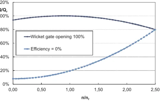
The curve atG =100% (i.e. fully open wicked gate) is reported in Fig. 4, together with the curve at
η=0%, so that the operating region allowed for the Francis turbine is defined. The water flow rateQ
can be calculated by means of Eq. (15) for any operating point, as a function of the current rotational speednand wicked gate openingG.
0% 20% 40% 60% 80% 100% 120%
0,00 0,50 1,00 1,50 2,00 2,50
Q/Qr
n/nr
Wicket gate opening 100%
Efficiency = 0%
Figure 4.Non–dimensional water flow rateQ/Qrvs. non–dimensional rotational speedn/nr.
For the sake of simplicity, the turbine efficiency is assumed constant and equal to the rated value
ηr (i.e. 90%). To account for the efficiency variation with the electric load, the turbine efficiency
may be expressed as a function of non–dimensional rotational speed (not considered in this paper). The non–dimensional turbine torque M is given by Eq. (16), as a function of the water flow rate Q, the water levelHand the rotational speedn. According to the dependencies shown in Eq. (15), the turbine torqueMis a function of the water flow rateQ, the rotational speednand wicked gate openingG.
M Mr
=
Q Qr
H Hr
n nr
= f2(Q,n,G) (16)
Finally, as in [15], the relations of Eqs. (17) – (20) express all the non–dimensional parameters in terms of the corresponding relative deviations. Note that, from the definition provided in Eq. (20), only negative values are allowed fory.
Q Qr
= 1+qt (17)
H Hr
= 1+ht (18)
n nr
= 1+x (19)
where qt represents the turbine flow rate relative deviation, ht the turbine water pressure relative
deviation, x the turbine speed relative deviation, and y the wicket gate servomotor stroke relative deviation.
With reference to the generator unit and its network, if the generator unit supplies for an isolated load, then the dynamic process of the generator unit considering the load characteristic is represented as:
x mt−mg0
= 1
Tas+eg (21)
wheremg0is the load torque,Tathe generator unit mechanical time, andegthe load self–regulation
factor.
In classic hydroelectric plants, conventional PID control laws are applied to control the hydraulic turbine speed, where the control signaluis the sum of three elements of proportional, integral, and differential gain of hydraulic turbine speed deviation (error)x, which can be thus expressed as:
u=x
Kp+ Ki
s + Kds
1+Tns
(22)
where Kp represents the proportional gain, Ki the integral gain, Kd the derivative gain, Tn the
derivative filter time constant. Section4will analyse and compare the performance of this standard PID regulators designede.g. in [13] with respect to the alternative control strategy proposed in this paper and described in Section3.
Finally, with reference to the servomechanism of the process, by neglecting small time constants, the relationship between the control signaluand the wicket gate servomotor strokeycan be expressed with a first–order equation:
y u =
1
Tys+1 (23)
whereTyis the wicket gate servomotor response time.
These expressions describe the nonlinear models of a typical hydroelectric power plant with two surge tanks and a Francis turbine, as shown in Fig.3.
2.3. Wind and hydraulic model comparisons
There is a stark contrast in the modelling focus within the wind and hydraulic communities. For wind turbines, the static relationship between the optimal rotation speed, pitch angle and incident wind speed is well understood and is enumerated for each wind turbine. In the hydraulic case, there is a complex dynamic relationship between the free surface elevation and the device motion. As a result, models for wind turbines focus more on the turbine mechanics, rather than the aerodynamics. In the hydraulic case, considerable effort is expended on accurately modelling the hydrodynamics of the system and, in contrast, there are a relatively small amount of studies with modelling the control section, which forms part of the lower control loop in Fig. 5. No doubt, one of the reasons for such a lack of generic hydraulic models is the lack of convergence or standardisation of control systems for hydroelectric devices. In addition, few devices have reached the stage of full scale prototype and, in many of those cases, most attention is focussed on the physical system design, with the control aspects receiving secondary attention.
3. Control Strategies for Energy Conversion Systems
Since Sections2.2and2.1have already recalled the basic and most common control solutions for wind turbines and hydroelectric systems, Section3.1focusses mainly on general control issues and preliminaries.
3.1. Background to Control Strategy Development
In general, control science attempts to devise algorithms that force a system to follow a desired path, objective, or behaviour modality. Traditionally, the control problem is defined by a tracking problem, where the objective is for the system output to follow the reference input [17]. While problems of this type do occur in energy conversion applications, for example speed control of both wind and tidal turbines, it is useful to broaden the set of problem descriptions and potential solutions a little, in order to assess the potential of control engineering in the general energy conversion context. In general, the control problem definition requires the maximisation or the minimisation of a prescribed performance objective (such as the max. energy, min. error) subject to proper system constraints (see e.g. amplitudes, rates, forces, etc) i.e. a constrained optimisation problem. The definition considered here is not inconsistent with the purpose of a classic controlled system with a feedback loop, where the objective function is usually some measure (e.g. a quadratic measure) of the difference between the controlled output and its desired value, i.e. the tracking error, with respect to the reference or the set–point. In this way, the desired performance of the tracking system in closed–loop can be specified in a variety of ways [17]:
1. Desired transient response; 2. Desired steady–state response;
3. Desired closed-loop poles (roots of the closed–loop transfer function); 4. Trade–off between control energy and tracking error;
5. Minimisation of the sensitivity of the closed–loop system to variations in the system description; 6. Minimisation of the sensitivity of the closed–loop system to external disturbances.
Items5and6in the list above relate to the system robustness and specific control methodologies to address these objectives have been developed since the late 1970’s. In most cases, control design methods provide an explicit solution for the feedback controllers, while some methods solve the more general optimisation problem defined at each time step. In the following, specific or general solutions, which can be useful in the control of wind turbines and hydroelectric systems, will be recalled and analysed.
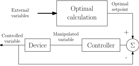
The general control problem framework is considered here, as shown in Fig. 5, consisting of an upper (optimal) setpoint generation stage and a lower control loop to ensure tracking of the setpoint. Both sets of control calculations must be mindful of physical constraints in the system. In the wind energy case, for variable speed turbines, an optimal rotational speed is first calculated (for Regions 2–3 of the power curve in Fig.2), and torque and/or blade pitch control used to achieve the required rotational speed. In the hydroelectric system case, an optimal velocity reference is calculated for a plant, and the regulation system allows to follow the desired velocity setpoint.
Optimal
calculation
Controller
Externalvariables
+
-Optimal setpointΣ
Controlledvariable
Device
Manipulated variable
Figure 5.General control structure with optimal setpoint calculation and servomechanism.
nonlinear controller. Significant care and attention must also be paid to adaptive schemes to ensure stability and convergence over all operating regimes [19].
3.2. Advanced Control Methodologies
This section recalls different control strategies including the standard PID controller, as well as Artificial Intelligence (AI) techniques, such as fuzzy logic, adaptive, and model predictive controllers, which are used for the regulation of the considered energy conversion systems. These methodologies are briefly outlined in the following, and compared in Section4.
The general description of the controlled system can be represented by the nonlinear dynamic functionF:
u(t) =F(x(t)) (24)
wherexis the process output,urepresents the control input, andtis the time. The control strategy applied to the system should determine the control inputu(t)such that the controlled process output x(t)is able to track a given reference or set–pointr(t).
It can be shown that a continuous–time linearised state–space description of the controlled system can be described by the general model of Eq. (25):
( ˙
xs(t) = Asxs(t) +Bsu(t)
x(t) = Csxs(t) (25)
wherexs ∈ <nwith a suitable ordernrepresents the state–space vector for the models described in
Section2. The matrices As,Bs andCs of the state–space model have appropriate dimensions. With
reference to the model of Eq. (25), the vectorx(t)represents the controlled outputs, whilst the vector u(t)is the controlled inputs.
The remainder of this section recalls different advanced control strategies including the standard PID controller, as well as AI techniques, such as fuzzy logic, adaptive, model predictive controllers, which are used for the regulation of the systems described in Section2.
Standard PID regulators are the most commonly used feedback controllers for industrial processes. The control logic is based on the computation of the errore(t)between the desired and the measured values of the output, i.e. e(t) = r(t)−x(t), which is fed back to the system after proportional, integral and derivative operations. In this way, the continuous–time control law of the PID regulator is described by Eq. (26):
u(t) =Kpe(t) +Ki
Z t
0 e(τ)dτ+Kd de(t)
dt (26)
whereKp, Ki,Kd are the PID proportional, integral, and derivative gains. The optimal selection of
balances the performance (response time) and the robustness (stability margins) of the controlled system [20].
The PID automatic tuning Simulink toolbox uses the linearised model of Eq. (25) of the energy conversion systems considered in this work.
Fuzzy Logic Controllers (FLCs) are extensively used in processes where the system dynamics are either very complex or exhibit highly nonlinear characteristics. The controller design approach relies on the identification of transparent rule–based Takagi–Sugeno (TS) fuzzy models using an Adaptive Neuro–Fuzzy Inference System (ANFIS) tool implemented in the Simulink toolbox. The same authors have already proposed the use of fuzzy regulators for the problem of the fault tolerant control design as shown in [21].
The TS fuzzy model consists of a set of rules Ri, where the consequents are deterministic
functionsfi:
Ri :IF x is AiTHEN ui= fi(x) (27)
withi = 1, 2, . . . ,KandKis the number of clusters or rules of the rule–based system,xrepresents the input vector of theantecedentvariables, anduidescribes theconsequentoutput. Airepresents the
antecedent fuzzy set of thei–th rule, defined by its (multivariable) membership functionµAi(x) → [0, 1]The function fiis represented by suitable parametric models, whose structure remains equal in
all rules, whilst the parameters can vary. A parametrisation in affine form is usually exploited, and described by Eq. (28):
ui=aix+bi (28)
where the vectoraiand the scalarbiare thei–th submodel parameters. The vectorxcontains a suitable
numbernof delayed samples of the model inputs and output. In this way, the productaixrepresents
an Auto–Regressive eXogenous (ARX) parametric dynamic model of ordern.
The final outputuof the TS fuzzy model is the weighted average of all rule outputs, computed as:
u= ∑
K
i=1 µAi(x)yi(x)
∑K
i=1 µAi(x)
(29)
The modelling approach used by ANFIS is similar to many system identification techniques. First, the TS fuzzy model structure described by the its ordern, the form of the membership functionsµAi
and the number of clustersKare hypothesised. Next, the input–output data are used by ANFIS for training the TS model according to a chosen error criterion, thus determining the optimal values of the controller parametersaiandbi[22].
The paper considers also an alternative approach to ANFIS for the derivation of the controller fuzzy model, which is represented by the Fuzzy Modelling and Identification (FMID) toolbox developed in the Matlab environment [22]. Also in this case, the estimation of the controller prototype relies on the identification of rule–based fuzzy models and using the input–output data acquired from the controlled process. This method exploits Takagi–Sugeno fuzzy models and employs the Gustafson–Kessel clustering method to divide the data into subsets with a common local linear (affine) behaviour [22].
The identified fuzzy controller is thus obtained by selecting an proper model structuren and a number of clustersK. The FMID toolbox provides the parametersai,bi and the estimation of the
membership functionsµAi of the optimal controller minimising the tracking errore(t).
The adaptive control method exploited in this paper is based on the on–line identification of a second order discrete–time transfer function of an ARX time–varying model in the form:
G(z) = b1z
−1+b 2z−2 1+a1z−1+a2z−2
(30)
whose parameters are recursively estimated at each sampling timetk = k T, withk = 1, 2, . . . , N,
N the number of samples, and T the sampling interval. z represents the unit advance operator. The parameters in Eq. (30) are estimated using the Recursive Least–Square Method (RLSM) with directional forgetting factor [20]. The same authors have proposed similar approaches but for fault tolerant control applications, as shown in [23].
The synthesis of the adaptive control law is derived using a modified Ziegler–Nichols criterion, in the form of Eq. (31):
uk=q0ek+q1ek−1+q2ek−2+ (1−γ)uk−1+γuk−2 (31) whereekis the tracking errore(t)at the sampling timetk,ukthe control signalu(t)at the sampling
timetk, whilstq0,q1,q2, andγare the time–varying controller parameters, which are calculated by
solving a Diophantine equation that leads to the following relations [20]:
q0= b11 (d1+1−a1−γ),γ=q2ba22 q1= ab22 −q2
b 1
b2 −
a1
a2 +1
,q2= sr11
(32)
wherer1= (b1+b2) a1b2b1−a2b12−b22
ands1=a2 ((b1+b2) (a1b2−a2b1) +b2(b1d2−b2d1−b2)). It is assumed that the final closed loop model has a behaviour similar to a second–order continuous time system with characteristic polynomials2+2δ ωs+ω2, whereδand ωrepresent its damping
factor and natural frequency, respectively. In this case, ifδ ≤ 1,d1 = −2e−δ ωT cos
ωT √
1−δ2
andd2=e−2δ ωT.
Both the on–line identification procedure and the adaptive controller parameter computation are implemented in the self–tuning controller Simulink library [20]. In this way, the sampled output yk of the time–varying ARX model of Eq. (30) should follow the sampled reference signalrk when
regulated by the control law of Eq. (31).
Note finally that, also in this case, the adaptive controller of Eq. (31) is connected to the continuous–time nonlinear system of Eq. (24) using the D/A and A/D converters.
Model Predictive Control (MPC) relies on dynamic models of the process, most often linear models obtained by system identification or linearisation of a nonlinear plant. The main advantage of MPC is the fact that it allows the current sampling time to be optimised, while keeping future sampling times in account. This is achieved by optimising a finite time–horizon, but only implementing the current sampling time. MPC has the ability to anticipate future events and can take control actions accordingly. PID controllers do not have this predictive ability. MPC is nearly universally implemented as a digital control.
MPC is based on iterative, finite–horizon optimisation of the plant model. At the samplek(k=
1, 2, . . . ,N) the current plant output is sampled and a cost minimising control strategy is computed (via a numerical minimisation algorithm) for a relatively short time horizon in the future:
k,k+Np.
Specifically, an online calculation is used to explore state trajectories that emanate from the current state and find (via the solution of Euler–Lagrange equations) a cost–minimising control strategy until timek+Np. Only the first step of the control strategy is implemented, then the plant state is sampled
An example of a cost functionJfor optimisation is given by:
J=
k+Np
∑
k
wxk (rk−xk)2+ k+Nc
∑
k
wuk∆u2k (33)
where wxk the weighting coefficient reflecting the relative importance of the monitored output xk,
andwuk the weighting coefficient penalising relative big changes in uk, with ∆uk = uk−uk−1. Np
represents the prediction horizon, whilstNcthe control horizon.
Note finally that the discrete–time MPC design is performed by using the MPC toolbox in the Simulink environment, which computes a linearisation of the hydroelectric nonlinear model of Eq. (25). The discrete–time MPC is thus connected to the continuous–time nonlinear system under investigation using the D/A and the A/D converters. The MPC Simulink toolbox uses the linearised model of the considered energy conversion systems.
3.3. Comparisons and Contrasts of Wind and Hydraulic Control Systems
Given the mature development of models of wind turbines and hydroplants, more attention has been focussed on the control problem, resulting in refined control systems which can undertake a variety of functions, including:
• Optimal set–point generation;
• Turbine speed and torque control (setpoint following);
• Supervisory control of the turbine, considering the different operation requirements under the various scenarios in Fig.2.
In addition, two advanced control strategies, such as data–driven and adaptive control, have also been considered for comparison purposes, as articulated in Section3.2.
It is clear that various ‘levels’ of control are required in both hydraulic energy and wind turbine applications. There is a top level of supervisory control which assesses the incident energy resource and may curtail the operation of the device in the face of extreme conditions. Such curtailment may be requirement in order to preserve the device integrity, ensure safe operation, or be required by legislation, as in the case of wind turbines. This is the case when wind turbines work in full load conditions, i.e. above the rated wind speed. On the other hand, they are designed to operate in the energy capture mode,i.e. below the rated wind speed. This working condition is similar to the hydroelectric systems, where maximum–energy transfer is required. However, hydraulic devices will frequently encounter states which are outside their normal operational envelope and some supervisory strategy may be necessary to ensure that device integrity is retained. Such supervisory control is important, and it can represent an important issue also for the safety of wind turbines, as discussede.g.in [21], but it will not be addressed in this work.
In an ideal world, one should consider the design of a complete system from the top down. However, convention has it that physical systems are usually designed by the discipline–specific experts and the control problem is then addressed in a subsequent step by control engineers, working in collaboration with the discipline–specific experts. Such an approach, though prevalent in the bulk of industrial applications of control, is non–optimal.
With reference to hydroelectric systems, the interaction between the optimal design of the hydroplant and the accompanying control system can represent the key point. The results suggest a strong interaction between the type of control system used and the optimal hydraulic device configuration, with optimal energy capture as an objective. For large–scale hydroelectric applications, control systems can offer performance benefits. Assuming that the prime energy converter is designed first, the addition of control can offer significant energy capture enhancement. There are close similarities with wind turbine control, one notable difference being that the density of the medium is about 1000 times greater in the case of hydroelectric systems. Wind turbine control highlighted that a variable–speed turbine is more efficient than the fixed–speed counterpart, but it requires proper torque and speed control, thus absorbing more energy. In the case of hydraulic energy, the numbers are more dramatic. It was shown that simple PID control has a relatively simple implementation of the more complex adaptive control, thus suggesting that energy capture can increase by as much as a factor of 4 with control in time–varying hydraulic systems, as highlighted in Section4.
4. Simulation Results and Comparisons
This paper considers the different control methods described in the previous sections to regulate the outputs of both the wind turbine and hydroelectric nonlinear systems recalled in Section2. The simulations are performed in the Simulink environment and using the toolboxes described above. The achieved results are compared in terms of percent Normalised Sum of Squared Errors (NSSE%), defined as:
NSSE%=100 v u u t∑
N
k=1(rk−xk)2
∑N
k=1r2k
(34)
whererkandxkrepresent the samples of the continuous–time signalsr(t)andx(t), respectively. The
simulation models of the wind turbine plant and the hydraulic system with two surge tanks and a Francis turbine described in Section2allow the simulation of the behaviour of both the processes in the presence of variable wind speedv(t)and large hydraulic transients after full load rejectionmg0, respectively. Usually, the most challenging working conditions for wind turbines occur in partial load, even if the full load case is also reported for comparison purpose. On the other hand, severe hydraulic transients happen after full load rejection.
As remarked in Section 2, the baseline control schemes for both the wind turbine and the hydroelectric systems use standard PID regulators, whose complete structure has been recalled in Section3.2. The optimal proportional and integral gains are determined using the automatic PID tuning procedure and settled toKp =0.6567,Ki =0.4468,Kd= 1.6567 for the hydroelectric system.
On the other hand, the optimal PID parameters for the wind turbine model are fixed toKp =4.0234,
Ki =1.0236,Kd=0.0127.
hydraulic turbine, the start–up phase is assumed to last 300 s (due to the large size of the considered Francis turbine), while the shutdown maneuver takes just 30 s, to simulate an unplanned emergency shutdown.
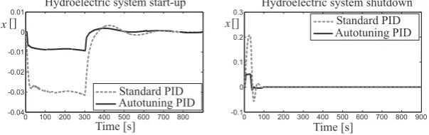
As an example, with reference to the hydroelectric system, the results reported in Fig. 6show that the PID governor of Eq. (26), whose parameters were optimised according to the PID autotuning Simulink toolbox, is able to keep the relative deviation of the rotational speed null (r(t) =0,i.e. the rotational speed constant) in steady–state conditions. Its performances are better than the standard PID regulator designed in [13]. Fig. 6 shows the turbine speed relative deviations x when the load torque mg0 changes in start–up and shutdown conditions. The hydroelectric system output is controlled by the continuous–time PID regulator, as shown in Fig.6with a simulation time of 900s.
Hydroelectric system start-up
Time [s]
0 100 200 300 400 500 600 700 800 -0.04
-0.03 -0.02 -0.01 0 0.01
Standard PID Autotuning PID
x[]
Time [s]
Hydroelectric system shutdown
0 100 200 300 400 500 600 700 800 900 -0.1
0 0.1 0.2 0.3
Standard PID
x
Autotuning PID []
Figure 6.Hydroelectric system with the PID regulator and automatic tuning.
Table1summarises the achieved results in terms ofNSSE% for the most severe conditions of load torquemg0(i.e.start–up and shutdown). According to these simulation results, good properties of the proposed autotuning PID controller are highlighted, and they are better than the PID governor [13]. In fact, the autotuning design is able to limit the effect of high–gains for the proportional and the integral contributions of the PID control. The same remark holds also for the wind turbine system, when the baseline PID controllers recalled in Section2are compared with the PID regulators with autotuning [10,11].
Some further comments can be drawn in general regarding the capability of these autotuning solutions. TheNSSE% values are lower in case of significant transient maneuvers (i.e. start–up and shutdown). On the other hand, with reference to the wind turbine system, good results are obtained also in this case. Note that standard industrial controllers, such the PID recalled in Section2, are quite simple and have the benefit of quite straightforward implementation. However, when applied to the control of nonlinear systems, the control laws cannot be very efficient. Therefore, the use of more advanced controller solutions can be motivated, as highlighted in the following.
With reference to the strategies described in Section3.2, fuzzy identification is used to derive the models of the controllers by exploiting the so–called model reference control approach [25]. For this purpose, the PID regulators designed for both the wind turbine and the hydraulic systems represent the reference controllers for the generation of the data used by the identification strategy described in Section3.2. In this way, the fuzzy controller parameters are identified such that the performances in terms of tracking errore(t)are optimised.
In particular, with reference to the TS fuzzy controller derived with the tools recalled in Section
3.2, a sampling intervalT=0.01s. is exploited and applied to the wind turbine system. Moreover, the fuzzy controller of Eq. (29) uses a numberK =3 of Gaussian membership functions, with a number of delayed inputs and outputn = 2. The antecedent vector is thusx = [ek,ek−1,ek−2,uk−1,uk−2]. The achieved performances of the controller when applied to the wind turbine system in partial and full load conditions are shown in Fig. 7. The fuzzy tools also provide the optimal estimate of the shapes of the membership functionsµAi. The achieved results are represented in Fig.7.
In particular, Figure7 shows the comparison between the reference outputs Pg(t) and ωg(t),
0 500 1000 1500 2000 2500 3000 3500 4000 0 1 2 3 4 5 6x 10
6
Pg(t)
Time (s.)
0 500 1000 1500 2000 2500 3000 3500 4000 40 60 80 100 120 140 160 180 w(t) g Time (s.) [W]
Generator power with fuzzy controller
[rad/s]
Generator speed with fuzzy controller
Measurement Set-point
Measurement Set-point
4400 4400
Figure 7.Controlled outputs of the wind turbine system compensated by the fuzzy regulators.
are reported in Table1, which are computed for the fuzzy controllers. The simulation results also highlight better properties of the proposed fuzzy controllers with respect to the standard PID with autotuning. This is motivated by the better capability and flexibility of the fuzzy tool, and in particular the FMID toolbox proposed in [22].
On the other hand, by considering the on–line procedure recalled in Section3.2, Fig.8shows the tracking capabilities of the adaptive controller of Eq. (31) applied again to the wind turbine system. The time–varying parameters of the adaptive control strategy have been obtained via the relations of Eqs. (32) with the damping factor and the natural frequencyδ=ω=1. The results achieved by the
adaptive regulation implementation using the Self Tuning controller Simulink Library (STCSL) are reported Fig.8over a simulation time of 4400s.
0 500 1000 1500 2000 2500 3000 3500 4000 0 1 2 3 4 5 6x 10
6
Pg(t)
Time (s.)
0 500 1000 1500 2000 2500 3000 3500 4000 40 60 80 100 120 140 160 180 w(t) g Time (s.) [W]
Generator power with adaptive control
[rad/s]
Generator speed with adaptive control
Measurement Set-point
Measurement Set-point
4400 4400
Figure 8.Controlled outputs of the wind turbine system compensated via the adaptive strategy.
Also in this case, Table1summarises the achieved results of the adaptive controller in terms of NSSE% considering a simulation time of 4400sand a sampling timeT = 0.01s. According to these simulation results, good properties of the proposed adaptive controller are highlighted, and they are better than both the autotuning PID regulators and the fuzzy controllers.
Finally, with reference to the MPC strategy recalled in Section3.2, the example of the reference and the monitored output signals are depicted in Fig.9for the hydroelectric system over a simulation interval of 900s. The control design uses a linearised state–space model of ordern =6. On the other hand, the state–space model for the wind turbine system has ordern=5.
The results shown in Fig. 9 have been achieved by using a prediction horizonNp = 10 and a
control horizonNc = 2. The weighting parameters have been settled towyk = 0.1 andwuk = 1, in
order to reduce abrupt changes of the control input. Also in this case, the MPC strategy performances for both the wind turbine and the hydroelectric systems are summarised in Table1.
Hydroelectric system start-up
Time [s]
0 100 200 300 400 500 600 700 800 900
-0.04 -0.03 -0.02 -0.01 0 0.01
x
MPC scheme Autotuning PID
[]
Time [s]
Hydroelectric system shutdown
0 100 200 300 400 500 600 700 800 900
-0.1 0 0.1 0.2 0.3
x
MPC scheme Autotuning PID
[]
Figure 9.Controlled output of the hydroelectric system compensated by the MPC law.
Table 1.Performance of the considered control solutions.
System Working Standard Autotuning Fuzzy Adaptive MPC
Model Condition PID PID PID PID Scheme
Wind turbine Partial load 36.89% 26.17% 13.56% 10.03% 7.23% system Full load 17.24% 9.87% 9.43% 7.67% 4.98% Hydroelectric Startup 15.86% 9.15% 7.32% 5.15% 3.76% system Shutdown 12.34% 8.57% 6.63% 4.78% 2.89%
Note that the MPC regulator can lead to quite good results, as its parameters are automatically tuned in the Simulink environment in order to optimise the MPC cost function of Eq. (33), as recalled in Section3.2.
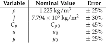
The remainder of this section analyses the robustness features of the considered controllers with respect to parameter variations of the system models. This analysis exploits the Monte–Carlo tool, as the control performance depends on the model–reality mismatch, as well as on the input–output measurement errors. Therefore, the analysis has been performed by describing both the wind turbine and hydraulic system model parameters as Gaussian stochastic processes with mean values corresponding to the nominal ones and and standard deviations corresponding to realistic minimal and maximal error values of Table2for the wind turbine model.
Table 2.Wind turbine model variable uncertainty.
Variable Nominal Value Error ρ 1.225 kg/m3 ±25% J 7.794×10⁶kg/m2 ±30%
Cp Cp0 ±45%
u u0 ±25%
y y0 ±25%
Moreover, it is assumed that the input–output signalsuandyof the wind turbine model and the power coefficient mapCpof Eq. (1) was affected by errors, expressed as per–cent standard deviations
of the corresponding nominal valuesu0,y0, andCp0also reported in Table2.
Also the hydroelectric simulator developed in the Simulink was able to statistically change the parameters of the model in order to introduce possible parameter variations. Under this assumption, Table3summarises the hydraulic system variables with their nominal values [26]. These nominal values of hydraulic system parameters have been varied by ±30% to perform the Monte–Carlo analysis.
Table 3.Hydroelectric model variable uncertainty.
Variable a b c Hf1 Hf3 Hf5 Ta
Nominal value -0.08 0.14 0.94 0.0481m 0.0481m 0.0047m 5.9s
Variable Tc Ts2 Ts4 Tw1 Tw3 Tw5
Nominal value 20s 476.05s 5000s 3.22s 0.83s 0.1s
Table 4.Sensitivity analysis for the considered control solutions.
System Working Standard Autotuning Fuzzy Adaptive MPC
Model Condition PID PID PID PID Scheme
Wind turbine Partial load 39.98% 29.67% 15.22% 12.33% 9.76% system Full load 18.56% 11.54% 11.89% 9.78% 6.43% Hydroelectric Startup 17.23% 11.33% 8.56% 7.04% 4.97% system Shutdown 14.12% 10.23% 7.98% 5.99% 4.04%
It is worth noting that, with reference to the values summarised in Table4 achieved via the Monte–Carlo analysis, they can serve to compare the overall behaviour of the considered controllers. Moreover, the values in Table4 suggest that when the modelling of the dynamic systems can be taken into account, the MPC scheme is preferred, even if an optimisation procedure is required. However, in the case of a system with modelling errors, after a certain amount of off–line learning, the fuzzy–based estimation error can fall below the value of the model–based schemes, as shown for the controllers derived via the automatic tuning procedure. On the other hand, fuzzy controllers achieve good control capabilities. The adaptive approach takes advantage of its improved features, as it is able to track possible variations of the controlled systems, but with quite complicated and not straightforward design procedures. The fuzzy–based schemes rely on the learning accumulated from off–line simulations, but the training stage can be computationally heavy. Regarding the standard PID control strategy, it is rather simple and straightforward, even if the achievable performances are quite limited.
4.1. Final Considerations
While control systems are ostensibly added in order to maximise power capture, care must be taken that such control systems have no adverse effect on the system. Though raw wind and hydraulic energy are essentially free, the systems to convert this raw energy are not and, ultimately, the receipts from energy sales are balanced to some extent by significant capital and operational costs. In the offshore environment, it is estimated that capital and operational costs are in roughly equal proportion. One important aspect in this economic perspective is to consider if the addition of a control system may drive the system more aggressively in an attempt to increase energy capture, perhaps leading to shortened device lifetimes. While the addition of control to a wind turbine is likely to be relatively benign, the use of motion–exaggerating control for a hydroelectric system can have a dramatic effect on the device lifetime. Consequently, the balance between increased energy capture (income) and increased device wear (cost) needs to be carefully considered.
relating to the design of control systems which are tolerant (in some respect, but sometime with reduced performance) to disturbance, model uncertainty, and measurement errors.
It has also been shown that there is often significant interaction between the optimal (uncontrolled) device design and the control system used to optimise its behaviour. For example in the hydrodynamic context, where controllers are effectively used to extend the bandwidth of the systems, so they can operate effectively across a wide variety of dynamic conditions, the uncontrolled system should be carefully designed, so that the controller can take maximum advantage. In both cases, significant advances in turbine control have led to a situation where turbine developers are providing progressively less control power, so that control energy consumption is minimised. However, this reaction, in turn, leads to highly nonlinear control action, since the control signals are regularly saturating, increasing the control challenge still further [27]. Moreover, the main challenges of modelling and control for wind turbines and hydroelectric systems have been highlighted. In order to present common and different requirements over power conversion efficiency (i.e. the renewable source power that can be converted into electric energy, the work exploited commonalities and contrasts for these two fields, that was mainly performed according the items below:
• System models description;
• Baseline controllers design;
• Advanced control strategies development.
On the basis of these items, the following considerations have been finally outlined. On one hand, wind turbine systems seem relatively mature from the modelling point of view, whilst hydroelectric systems still present challenging control issues. This remark is valid for medium size wind turbines: large rotor installations can drive challenging and complex modelling and control issues.
Both wind turbine and hydroelectric systems can share a common structure. In addition to these components, a further level of supervisory control is required to correctly select the control strategy appropriate to the model of operation, usually dictated by the prevalent resource measure. For the wind turbine case, such operational modes are well defined, as articulated in terms of the various sections of the power curve. However, though the overall number of operational modes may be lower, hydroelectric systems also have a cut–in power level below which energy conversion is not economic/possible, a main power production region where energy conversion should be maximised, a region where energy conversion must be curtailed due to the capacity of (for example) electrical components and, finally, a survival mode where energy production is abandoned and system motion configured to avoid potential structural damage. The means by which survivability is managed in the hydraulic case is not as straightforward as in wind, due to the wide variety of hydraulic devices and the difficulty of finding an orientation or configuration which avoids the destructive influence of hydraulic energy fluxes.
Despite the differences in relative maturity of wind and hydraulic energy, both share many fundamental principles, including the fact that only a fraction of the raw wind and hydraulic resources can be usefully converted, at best. These limitations relate to basic aerodynamic (wind) and hydrodynamic (hydraulic) considerations.
In general, both hydraulic and wind energy conversion systems require a high degree of availability, as it significantly affects the final energy cost. Moreover, these systems have highly nonlinear dynamics, with stochastic inputs, in the form of driving forces. Suitable control methods should provide the optimisation of the energy conversion efficiency over wider than normally expected working conditions. Moreover, it was shown that proper mathematical descriptions were necessary to capture the complete behaviour of the systems under consideration, thus providing an important impact on the control design itself.
from a modelling and control perspective, coupled with the high cost of offshore deployment and maintenance, helps to explain why medium–size wind turbines and micro– or pico– hydroelectric systems can be now commonplace, whilst very large devices are not.
5. Conclusion
The paper was motivated by the focus on utilising renewable energy resources in a bid to fulfil increasing energy requirements and mitigate the climate change impacts of fossil fuels. While most renewable resources are free, the technology used to usefully convert such resources is not and there is an increasing focus on improving the conversion economy and efficiency. To this end, the paper highlighted that advanced control technology can have a significant impact and is already a relatively mature technology for wind turbines. Though hydroelectric plants can use simple regulation systems, significant benefits have been shown to accrue from the appropriate use of the the same advanced control strategies proposed for wind turbine processes. This represented one of the key issues of the paper. In fact, to date, the application communities connected with wind and hydraulic energies highlighted little communication, resulting in little cross fertilisation of control ideas and experience, particularly from the more mature wind area to hydraulic systems. Therefore, taking into account differences between wind turbine and hydroelectric systems, this paper analysed the application of advanced control methodologies across both domains, both from a comparative and contrasting point of view, with the aim of identifying commonalities in control objectives and potential solutions. Key comparative reference points include the articulation of the models, specification of control objectives, development of realistic device models, and development of solution concepts. Not least, in terms of realistic system requirements are the set of physical and legislative constraints under which such renewable energy systems must operate, and the need to provide reliable and robust control solutions, which respect the often remote and relatively inaccessible location of many onshore and offshore deployments.
Acknowledgments: The research work has been supported by the FAR2016 local fund from the University of Ferrara. The costs to publish in open access will be covered by the FIR2016 local fund from the University of Ferrara.
Author Contributions: Silvio Simani analysed the methodologies, the achieved results, and together with Stefano Alvisi and Mauro Venturini, wrote the paper.
Conflicts of Interest:The authors declare no conflicts of interest.
Bibliography
1. Bianchi, F.D.; Battista, H.D.; Mantz, R.J. Wind Turbine Control Systems: Principles, Modelling and Gain Scheduling Design, 1st ed.; Advances in Industrial Control, Springer, 2007. ISBN: 1–84628–492–9.
2. Pao, L.Y.; Johnson, K.E. Control of Wind Turbines. IEEE Control Systems Magazine2011,31, 44–62.
3. World Energy Council., Ed. Cost of Energy Technologies; World Energy Perspective, World Energy Council: London, UK, 2013. ISBN: 9780946121304. Available at:www.worldenergy.org.
4. Odgaard, P.F. FDI/FTC wind turbine benchmark modelling. Workshop on Sustainable Control of Offshore Wind Turbines; Patton, R.J., Ed.; Centre for Adaptive Science & Sustainability, , 2012; Vol. 1.
5. Blanke, M.; Kinnaert, M.; Lunze, J.; Staroswiecki, M. Diagnosis and Fault–Tolerant Control; Springer–Verlag: Berlin, Germany, 2006.
6. Johnson, K.E.; Fleming, P.A. Development, implementation, and testing of fault detection strategies on the National Wind Technology Center’s controls advanced research turbines. Mechatronics2011,21, 728–736. DOI: 10.1016/j.mechatronics.2010.11.010.
7. Global Wind Energy Council. Wind Energy Statistics 2013. Report, 2014.
8. Burton, T.; Sharpe, D.; Jenkins, N.; Bossanyi, E. Wind Energy Handbook, 2nd ed.; John Wiley & Sons: New York, 2011.
10. Odgaard, P.F.; Stoustrup, J.; Kinnaert, M. Fault Tolerant Control of Wind Turbines – a Benchmark Model. Proceedings of the 7th IFAC Symposium on Fault Detection, Supervision and Safety of Technical Processes; , 2009; Vol. 1, pp. 155–160. DOI: 10.3182/20090630–4–ES–2003.0090.
11. Odgaard, P.F.; Stoustrup, J. Unknown Input Observer Based Scheme for Detecting Faults in a Wind Turbine Converter. Proceedings of the 7th IFAC Symposium on Fault Detection, Supervision and Safety of Technical Processes; IFAC – Elsevier: Barcelona, Spain, 2009; Vol. 1, pp. 161–166. DOI: 10.3182/20090630–4–ES–2003.0048.
12. Singh, R.R.; Chelliah, T.R.; Agarwal, P. Power electronics in hydro electric energy systems – A review. Renewable and Sustainable Energy Reviews2014,32, 944–959.
13. Fang, H.; Chen, L.; Dlakavu, N.; Shen, Z. Basic Modeling and Simulation Tool for Analysis of Hydraulic Transients in Hydroelectric Power Plants. IEEE Trans. Energy Convers.2008,23, 424–434.
14. Popescu, M.; Arsenie, D.; Vlase, P.Applied Hydraulic Transients: For Hydropower Plants and Pumping Stations; CRC Press: Lisse, The Netherlands, 2003.
15. Vournas, C.D.; Papaionnou, G. Modeling and stability of a hydro plant with two surge tanks. IEEE Trans. Energy Convers.Jun.,10, 368–375.
16. Betz, A.; Randall, D.G. Introduction to the Theory of Flow Machines; Permagon Press: Oxford, 1966. ISBN: 978–0080114330.
17. Kuo, B.C.Automatic Control Systems, seventh ed.; Prentice Hall: Englewood Cliffs, New Jersey, 07632, 1995. 18. Simani, S.; Fantuzzi, C.; Patton, R.J. Model-based fault diagnosis in dynamic systems using identification
techniques, first ed.; Vol. 1, Advances in Industrial Control, Springer–Verlag: London, UK, 2003. ISBN: 1852336854.
19. Ioannou, P.; Sun, J.Robust Adaptive Control; PTR Prentice–Hall: Upper Saddle River, NJ, USA, 1996. 20. Bobál, V.; Böhm, J.; Fessl, J.; Machácek, J. Digital Self–Tuning Controllers: Algorithms, Implementation and
Applications, 1st ed.; Advanced Textbooks in Control and Signal Processing, Springer, 2005.
21. Simani, S.; Alvisi, S.; Venturini, M. Fault Tolerant Control of a Simulated Hydroelectric System. Control Engineering Practice2016,51, 13–25. DOI: http://dx.doi.org/10.1016/j.conengprac.2016.03.010.
22. Babuška, R.Fuzzy Modeling for Control; Kluwer Academic Publishers: Boston, USA, 1998.
23. Simani, S.; Alvisi, S.; Venturini, M. Data–Driven Design of a Fault Tolerant Fuzzy Controller for a Simulated Hydroelectric System. Proceedings of the 9th IFAC Symposium on Fault Detection, Supervision and Safety for Technical Processes – SAFEPROCESS’15; IFAC., Ed.; IFAC: Paris, France, 2015; Vol. 48, pp. 1090–1095. DOI: 10.1016/j.ifacol.2015.09.672. ISBN: 978–3–642–27644–6. ISSN: 1474–6670. Special session invited paper. 24. Simani, S.; Alvisi, S.; Venturini, M. Fault Tolerant Model Predictive Control Applied to a Simulated Hydroelectric System. Proceedings of the 3rd International Conference on Control and Fault–Tolerant Systems – SysTol’16; Control Systems Society, I., Ed.; Research Center for Supervision, Safety and Automatic Control of the Universitat Politècnica de Catalunya in Barcelona, IEEE: Barcelona, Spain, 2016; pp. 251–256. ISBN: 978–5090–0657–1. ISSN: 2162-1209. DOI: 10.1109/SYSTOL.2016.7739759. Special session invited paper.
25. Brown, M.; Harris, C.Neurofuzzy Adaptive Modelling and Control; Prentice Hall, 1994.
26. Simani, S.; Alvisi, S.; Venturini, M. Study of the Time Response of a Simulated Hydroelectric System. In Journal of Physics: Conference Series; Schulte, H.; Georg, S., Eds.; IOP Publishing Limited: Bristol, United Kingdom, 2014; Vol. 570, Conference Series, pp. 1–13. ISSN: 1742–6596. DOI: 10.1088/1742-6596/570/5/052003.