cover. A few results are given in terms of frequency and of num- bers of plants and interpreted on a basis of percentage species composition. The data are gener- ally used in the evaluation of cbndition and trend of brush
ranges under the impact of
browsing or some type of manip- ulation. Pressure for more and better hunting of big game is en- hancing the value of browse and the need for efficient’ sampling techniques. At present the in- vestigator who is working on brushland problems must bor- row and modify the techniques used by the grassland ecologist and the forester. These modified methods have not undergone ex- tensive tests for accuracy and reliability. In fact reports of quantitative sampling in brush
for species composition are
scarce in comparison with the data available for grasslands and forests.
The purpose of this study was to compare for accuracy and practicability the techniques ‘of
1 The data from the Hopland Field Station were collected as a part of Project 1501 in the California Agri- cuZturaZ Experiment Station. The material from Madera County was from a project conducted coopera- tively by the University of CaZi- fornia and the California Depart- ment of Fish and Game under Fed- eral Aid in Wildlife,
Act Project California Game Investigations.
Restoration W-51R, Big
teristic of the vegetation that was measured in all three methods was area of the soil covered by the woody plants when their canopies were pro- jected perpendicularly to the soil surf ace.
One study area was located on the Hopland Field Station in southeastern Mendocino County, California and the other on the Lion Point area of the San Joa- quin winter deer range in Ma- dera County.
Related Studies
The first studies on shrubs used square or rectangular plots of varying sizes. The milacre was the most common. On these quardats ocular estimates of cover were made (Forsling and Storm, 1929; van Breda, 1937; Horton, 1941; and Sampson, 1944). In an attempt to reduce the inaccuracies of ocular esti- mates, Nelson (1930) suggested accurate charting of shrub can- opies by a two-man team with the aid of a tape and traverse board. Osborn, Wood, and Palt- ridge (1935) divided square plots into a grid with strings and charted canopies by measure- ments from the intersections.
Pickford and Stewart (1935)
used two parallel steel tapes to mark the boundary of a belt transect. They charted the can- opies by measurement of can- opies from a metal strip moved
180
The results indicated that the line intercept was probably more accurate than the quadrat and required less time. The line was much easier to use in woody veg- etation than the quadrat. Parker and Savage (1944) included shrubs in their study of the relia- bility of the line intercept method in measuring the vegeta- tion of the Southern Great Plains. The method was applied effectively in an extensive study of the creosote bush area along the upper Rio Grande Valley
(Gardner, 1951) and to study forage conditions on winter game range along the Salmon River in Idaho (Smith, 1954). Hedrick (1951) combined deter- minations of numbers of plants on milacre plots and intercepts to study succession on chamise areas following brush manipula- tion.
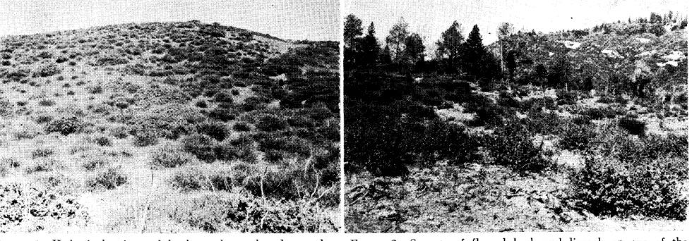
FIGURE 1. Hedged chamise and leather oak on the plot at the FIGURE 2. Sprouts of flannel bush and liveoak on one of the
Hopland Field Station. plots in Madera County.
Herd Committee, 1954).
Taber (1955) used a rope with 3-foot marks instead of a tape to sample heavy mature brush. The rope, with a weight on one end, was thrown across the top of the brush. The observer did not need to follow the transect exactly to read the points. These adapta- tions of the line point method greatly facilitated sampling in thick brush.
Met hods
In the Hopland area a plot of mixed brush 100 feet on a side was selected for study. The first step was to stake the corners. The second step was to map the canopy outlines of all woody plants at a scale of % inch on the map to 1 foot on the ground. In those cases where the canopy boundaries were not clear-cut an estimated boundary was drawn which excluded interspaces ex- ceeding 2 inches. This was not considered a serious source of variation before sampling but it may have contributed to some of the variation between species. The third step was to measure the intercept of shrub canopies along 20 lines, each 100 feet in length and located at IO-foot intervals in two directions across the plot. The fourth step was to take point plots at the foot markers along the tape by noting the hit of the point of a plumb bob suspended so that the sup-
porting string touched the tape. On the San Joaquin area two plots 100 feet on a side were se- lected in an area where a stand of mixed brush had been mashed and burned the preceding year. After the corners of the plots were established, intercept of shrubby vegetation was meas- ured along 40 lines 100 feet long and spaced at 5-foot intervals across the plot in both directions. Point plots were taken at each foot marker along the same lines. Data for each 5-foot segment of the lines were recorded sepa- rately, coded, and punched on IBM cards.
Time to read the field plots and to summarize the field sheets was recorded for part of the work in each area.
Composition of the Vegetation The general appearance of the Hopland plot is of separate bushes of chamise (Adenostoma fasciculatum), leather oak (Quercus durata), and wedgeleaf ceanothus (Ceanothus cuneatus). Hereafter it will be referred to as the chamise plot. Three other species; redberry (Rhamnus cro- tea), deer brush (Ceanothus in- tegerrimus), and manzanita (Arctostaphylos g2anduZosa) were present but very scarce. Most of the plants were under 3 feet in height and had been closely hedged by grazing ani- mals (Figure 1). The average
length of individual plant inter- cepts by the line transect method was 2.37 feet for chamise, 3.23 feet for oak, and 1.28 feet for ceanothus. Even though these intercepts do not represent aver- age crown diameters, they do give an approximate picture of relative plant width. The can- opies of some plants touched and intermingled so that areas of several square feet had contin- uous cover.
In terms of ground cover about 35 percent was covered by cham- ise, 8 percent by oak, and 6 per- cent by ceanothus. The others contributed less than one percent of the cover. The total cover was slightly over 50 percent. In terms of percentage species com- position, chamise was about 70 percent, oak about 16 percent, and ceanothus 12 percent (Table 1).
On the two San Joaquin plots the vegetation consisted of one- year-old brush sprouts and seed- lings (Figure 2). Interior live- oak (Quercus wislizenii), flan- nel bush (Fremontia californica), western mountain-mahogany
cuneatus 624.38 128.91 137
Rhamnus crocea 16.44 2.12 3
Ceanothus
integerrimus 3.24 0 0
Arctostaphylos
glandulosa 1.68 0 0
Total 5,107.70 1,012.97 1,018 -
12.23 12.73 13.45
0.32 0.20 0.30
0.06 0 0
0.03 0 0
100 100 100
the ground cover. These plots will be referred to as the liveoak plots. Plant size ranged from seedlings about 1 inch in diam- eter and 3-4 inches in height to clumps of interior liveoak sprouts 4 feet in height and 15 feet in diameter. Although the area had heavy use by deer and cattle, plant boundaries were usually very irregular due to the presence of long leaders on many of the young sprouts. Intermin- gling of the canopies caused the sum of the cover by species to exceed the total ground cover.
On one plot, ground cover was 24 percent and on the other 18 percent. In the first plot interior liveoak occupied 17 percent of the area, yerba Santa seedlings 3 percent, wedgeleaf ceanothus . seedlings 1 percent, and moun-
tain-mahogany almost 2 percent. The remainder of the ground cover was contributed by ten species each with less than l/2- percent cover (Table 2). On the second plot interior liveoak and flannel bush each occupied 7 per- cent. Twelve other species made up the remaining ground cover.
Line Transect, Line-point, and Charting Compared for the
Chamise Plots
The results from measuring
the vegetation by charting, line transects, and line point proce- dures in the chamise plot are shown in Table 3. There was very little difference in the means obtained by the different methods. All were within the confidence interval calculated at the 5 percent level for any one of the methods. It would seem that these different methods yielded means that were well within the limits required by most objectives in vegetational
sampling. The comparison of
the means gives little basis for choosing one of the methods as superior to the others. This same conclusion was reached in the comparison of the intercept and line point data from the liveoak plots.
The variance or standard devi- ation of sampling units was gen- erally much less in both the line transect and the line‘ point methods than with the charting method. The charted plots were more variable than the others. The standard error of the mean in each case was somewhat less conclusive in favor of any of the methods and further indicates that all methods gave accurate estimates of the population mean with the size of sample em- ployed. The coefficient of varia-
the number of plots required to
sample them adequately was
much greater than for the total cover.
Variation analysis and sample size calculations to obtain means within certain specified limits indicate that both transect methods were superior to chart- ing, Undoubtedly the reason is that the 100-foot lines cross local variations in cover which result in less difference between lines than was the case with plots lo- feet square. The principle of long narrow plots being better than square plots has been well established and is further strengthened by these results.
Paired Transects from the Field and Chart
For the line intercepts and the line points on the chamise plot, one set of data was taken in the field and another comparable set was obtained by sampling from the map of the study area. These two sets were taken in the same location and, therefore, were considered as paired obser- vation and analyzed on a basis of mean differences.
In all cases but one, sampling from the map gave larger num- bers for intercepts and points than sampling in the field. The differences were significant at the 99 percent level for the total cover by both intercepts and points and for chamise with the point method (Table 4).
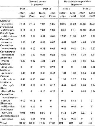
Table 2. Ground cover and percentage species composition obtained by line intercept and line points on two areas 100 by 100’ feet located on the San Joaquin winter deer range.
Ground cover in percent
Plot 1 Plot 2
Inter- Line Inter- Line
cept Point cept Point
Quercus
wislizenii 17.14
Fremontia californica Eriodictyon californicum Ceano thus
cuneatus Ceanothus Zeucodermis Cercocarpus betuloides R hamnus crocea Quercus douglasii Quercus kelloggii Prunus subcordata Lonicera interrupta Rhus diversiloba Ceanothus leucodermis- sprouts R hamnus californica Sambucus 0.14 17.17 0.10
3.07 2.82
1.16 0.11 1.54 0.39 0 0.45 0.48 0.11 0 1.40 0.10 1.40 0.32 0 0.45 0.55 0.12 0 0.10 0.11 0.12 0.12 0.05 0.05 coerulea 0.03
Arctostaphylos mariposa 0.03
7.27 7.08 0.07 0.88 0.38 0.26 1.33 0.76 0.48 0.01 0.12 0.16 0 0 0.04 0.03 7.35 7.20 0.01 0.87 0.40 0.22 1.30 0.72 0.42 0 0.12 0.20
Total 24.121 24.20 17.89 17.87
Botanical composition in percent
Plot 1 Plot 2
nter- Line Inter- Line
cept Point cept Point
68.95 0.56 12.35 4.67 0.44 6.20 1.57 0 1.81 1.93 0.44 0 69.32 0.41 11.39 5.65 0.41 5.65 1.29 0 1.82 2.22 0.48 0 0.48 0.48 0.20 0.20 38.53 37.52 0.37 4.66 2.01 1.38 7.05 4.03 2.54 0.05 0.64 0.85 0 0 0.21 0 39.07 38.28 0.05 4.63 2.13 1.17 6.91 3.83 2.23 0 0.64 1.06
i This is amount of ground covered by plant canopies and does not equal sum of the cover by species due to intermingling of plant canopies.
erage than actually occurred on the ground. The small t values for oak indicate that it was map- ped very accurately. This could be expected because the canopy boundaries were clear-cut and the foliage of broad leaves was closely packed on short branches
without interspaces. On the
other hand chamise had irregular and indefinite canopy bound- aries. Long branches protruding around the edges of each plant incompletely covered the ground so the investigator had to aver-
age the irregularities to 100 per- cent density by ocular means. This evidently resulted in cham- ise being mapped as an area slightly larger than it actually was. Ceanothus was intermedi- ate between the oak and chamise in these characteristics. Un- doubtedly, charting of shrubs is more accurate with some species than with others.
Further Comparisons of Line Intercepts and Line Points In the sampling of brush, as well as with other vegetational
types, decisions must be made on size, number, and location of
samples. These items were
studied with data from the live- oak plots. The analysis followed a procedure whereby the data for ground cover were accumu- lated in several different ways. As every successive increment was added the new sum was divided by the new sample size to give a series of means. The types of accumulation were: (1) forty 100-foot lines in the order in which they occurred in the field, (2) forty lOO-foot lines in a random arrangement, (3) 800 5-foot segment of lines in a ran- dom arrangement, and (4) 4,000 single line points in a random arrangement. The first three of these types of accumulations were done for both intercepts and points. The cover for each species and the total cover was accumulated separately for the two liveoak plots.
An example of the accumula- tion process is as follows: 242 hits were recorded for the first 1,000 randomly arranged points. The next 100 points with 19 addi- tional hits gave 261. The corre- sponding means for the l,OOO-and - l,lOO-point samples are 24.2 and 23.7 percent cover, respectively. These are two in series of accum- ulated means.
With the addition of the last group of points or lines, the final accumulated mean was obtained. The final mean for line intercept was used as the true population mean and deviation of each ac- cumulated mean from the pop- ulation mean was expressed as a percentage of the population mean and used to construct a series of graphs of which Figure 3 is one example.
Calculated n3 ~~ 43 -____ 10 9 87 14 16
Quercus durata Ceanothus cuneatus
_______- -
Mean ground cover 8.22 8.40 8.60 6.24 6.45 6.85
Standard error 1.248 1.288 1.183 0.843 1.253 1.425‘
Coefficient of variation1 151.83 68.57 61.64 135.01 86.79 93.02
Confidence intervals 52.45 k2.52 k2.32 t1.65 k2.46 k2.79
Calculated n3 885 181 146 702 290 333
_____
1 Coefficient of variation equals the standard deviation divided by the mean, expressed in percent.
2 Confidence intervals equals -c t .05 for infinite degrees of freedom multiplied by the standard error.
SCalculated sample size equals t2 Cs, where t is at 0.05, C is the coefficient _m
P”
of variation, and P is IO percent of the mean.
this deviation and does not de- note probability of error in the statistical sense.
With all of the species together and with single species having ground cover greater than 3 per- cent, the deviation of the accum- ulated means from the real mean showed very small differences between line intercepts and line points. This is illustrated for total vegetation at a cover of 24 percent (Figure 3)) and was true for several species on both plots. The parallel nature of the paired lines for points and intercepts suggests that the two procedures give similar results at various sample sizes.
With species having densities of 3 percent or less the diver- gence of accumulated means be- tween line intercept and line points for most of the sample sizes was large. This is illus- trated for wedgeleaf ceanothus seedlings at a ground cover of 1
percent (Figure 4) and was
found with the other species of low cover. With these species
there is little assurance that either points or intercepts give an adequate sample. However, the line intercepts exhibited less fluctuation and this method is probably the best for sampling the species with low cover.
Comparative results of the random and systematic methods of sampling is shown by the size
of sample required by each
method to bring the deviation of the accumulated means within the 5 percent level (Figures 3 & 4 and Table 5). When the data for total vegetation were ran-
points will give means little dif- ferent from line intercept at a reasonable sample size. With species of low cover, the percent- age variation between the points and intercepts is high and sam- ples must be large and would sel- dom be practical. Although there were inconsistencies, the trend was for the sample size necessary to reach the 5 percent level to decrease with random- ization of successively smaller sampling units.
In sampling, the practical as- pects as well as accuracy and precision must be considered. Randomization of samples can be accomplished by the use of co- ordinate lines but this would in- volve a great deal of work. It is difficult to move about in many brush fields.
Systematic sampling can be with lines several hundred feet in length. With this type of sam- pling the number of lines re- quired to sample within the de- sired level of precision would be larger than with any of the ran- dom methods. However, the ease
Table 4. Mean difference analysis for paired transe&s sampled in the
field and from the map of ground cover for fhe chamise plot.
Line points ____- Line intercepts
___-
Afal Ccu Qdu Total Afa Ccu Qdu Total
Mean difference 2.55 0.50 0.05 3.2 1.57 0.70 0.08 2.40
Greatest Map Map Map Map Map Map Field Map
Standard error 0.844 0.471 0.576 0.882 0.852 0.388 0.458 0.742
t.01 3.02”” 1.061 0.087 3.628”” 1.84 1.80 0.175 3.24””
Confidence
interval k1.76 _____ 21.84 -t-1.55
’ The species are Adenostoma fasciculatum, Ceanothus cuneatus, and Quer- cus durata.
FIGURE 3. Percentage deviation of accumulated means from the population mean for total vegetation on the liveoak plot with a density of 24 percent. Dotted lines on vertical planes show the 5 percent level of deviation. White lines across the base plane indicate sample sizes in feet or the ecprivalent number of points. See text for explanation of calculations.
of establishing and sampling such lines make them the more practical.
Field and Office Time Required by Transects The time required to read each line of intercepts and points in the field and the initial summar- ization of each in the office was recorded for the chamise plot. For both field recording and ini- tial summarization combined, the line point method took about one-third as much time as the line intercept (Table 6). Even though it was not recorded the time required to chart a lOO- square-foot plot was more than for a lOO-foot line of intercepts.
The point method had a great
advantage over the other
methods in office time. To tally the points required only a count, while the charting method neces- sitated measurements of areas with a planimeter, and the inter- cepts required summation. The
calculations were also much
easier with the point method be- cause whole numbers with two significant digits constituted the data, while with the other
methods mixed numbers were
used. The smaller numbers lend themselves to fewer errors in calculations than the larger numbers.
The time required to take a line of intercepts and of points at two brush densities in the live- oak area was determined by two operators. Each required over twice as much time to measure
the intercepts as the line points. When 5 minutes for line estab- lishment was added to the read- ing time, the ratio of time was 1.6 to 1.8 in favor of the points (Table 7). Density of the second line was 3 times that of the first, which resulted in a time increase for both methods by 20 to 50 per- cent.
When IBM cards are used to record the data, the fewer num- ber of digits necessary for line points necessitates fewer col- umns for a given unit of line and
more information may be
punched on each card. With
fewer cards less time and ex- pense are involved in punching, sorting and any other machine processing necessary.
The total time required in the field and office was closely re- lated to the number of plants in one case and the size of plants in another. On the chamise plots the correlation coefficient be-
tween numbers and time was
0.7878 for points and 0.6453 for intercepts. These were both sig- nificant at the 99 percent level. Larger sprouts rather than more plants resulted in more time per transect in the liveoak plots.
Even though analysis of the
Interior liveoak, ground cover-7.08
Percent 2,600 600 1,300 1,900
____-
1700 feet were required for line points. All other sample sizes were the same for points and intercepts.
variation and of differences be- tween sample means and popula- tion means did not indicate one of the transect methods to be superior, except at plant den- sities below 3 percent, an analy- sis of the time required in sam- pling marked the line point method as the one to use. If the same amount of time were put into both methods, the investi- gator would have a larger sam- ple with the line point technique and consequently a better esti- mate of the population.
Sample Size with Species of Differeni Cover and Distribution
In this as in most studies of vegetation, data were collected on several species. These species varied widely in foliage cover. Generally, the lower the cover, the greater the ratio of standard deviation to the mean and the larger the sample required
(Tables 3 and 5) .
An assumption of normality in
Table 6. Average time in minutes fo record each transect in the field
and to summarize field sheets
for the chamise plot
Line Line
points intercepts
Field time 7.81 16.18
Summary time 0.75 10.46
Total 8.56 26.64
_
the population being sampled is usually made although normality
may or may not exist. This is illustrated by an analysis of fre- quency distribution of crown cover by five percent classes in the chamise plot (Figure 5). The bar graphs show the actual fre- quencies for total cover and cha- mise and the calculated normal curves for a population with the
25
I
TOTAL OF ALL SPECIES
r 20
9
IS n
IO 20 30 40 50 60 70 60 Go 100 GROUND COVER IN PERCENT
population is normal. Both
curves are slightly skewed to- ward the higher density classes and slightly flattened.
For oak and ceanothus the dis- tributional curves of ground cover take an entirely different shape. With both, a large num- ber of plots had no plants and
with increasing cover there
were fewer plots. These distri- butions seem to fit paraboloid curves best.
Frequency of crown cover by 5 percent classes was determined for the liveoak plots. The distri- butions obtained were similar to
OUERCUS DURATA
25
ADENOST~MA FASCICULATUM
CEANOTHUS CUNEATUS
O 0 IO 20 30 GROUND COVER IN
400
PERCENT
Table 7. Time in minutes fo establish in the area of the liveoak plots.
fwo transects by two men
Percent Operator 1 Operator 2
density Gtercepts Points Ratio Intercepts Points Ratio _~
Line 1 18.37 18:06 11:30 1.6 23:35 13:05 1.8
Line 2 56.37 26:45 14:35 1.8 29:35 16:00 1.8
Ratio 3.1 1.5 1.3 1.3 1.2
those of the low-density species in the chamise plot. None ap- proached a normal distribution.
Frequency distributions are greatly influenced by the size of field plots and by the class inter- vals into which the plots are grouped. These data are shown to indicate only that each species exhibits a separate type of dis- tribution. Thus, each species constitutes a distinct population and combinations of species make still additional populations.
In this study of cover by sev- eral species and three totals, all but one species and one total ex- hibited extreme positive skew- ness in distribution. However, the seriousness of non-normality is not great because sample means from such populations are normally distributed about the population mean provided the number of items in the sam- ple is large (Feller, 1950; and Madow, 1948). The. nearly nor- mal distribution of 200 sample means of 20 random line points from the total cover of one live- oak plot illustrates this principle
(Figure 6).
The use of normal procedures with skewed data may lead to misinterpretation. Generally, wrong inferences about the pop- ulation mean will be concen- trated on one side of the, confi- dence belt. With great positive skewness, a large proportion of the wrong statements will be above the upper confidence limit. Another effect of non- normality is to produce high variability in the variance from one sample to another.
A sample which is based on the total cover, and is adequate or within the limits set by the
investigator as satisfactory, may not sample any of the individual species adequately. On the other hand, the number of plots needed to sample the species of lesser importance may be so great that the sampling is beyond the facil- ities of the investigation. The investigator must be aware of these difficulties in order to make an intelligent decision as to sample size and to draw only those conclusions warranted by the data. Few guide lines or rules of thumb can be established except through preliminary sampling of the population being studied.
Ordinarily an estimate of sam- ple size should be made for each item in the investigation. If the indicated n’s are close together, the investigator is fortunate and can proceed. If the n’s are some- what divergent, he has several choices of sample size. He may regard those items which are most important to him and dis- regard the others completely. Or, he may choose a size that will
over-sample some species in
order to get precise information on others. He also has available a choice of different sampling
FIGURE 6. Solid line is the frequency dis- tribution of 400 plots according to 5-per- cent-ground-cover classes of the entire brush cover on one of the liveoak plots. Dashed line is the frequency distribution of 200 sample means of 20 random points taken from the same population.
procedures for the different com- ponents of the vegetation. He may relax his standards of pre- cision or choose different ones for the different species.
The choice of these alternatives is one to be made by the investi- gator and is based on the objec- tives of his study and on the funds and time that he has avail- able. Cochran (1953) has given some guide lines that are help- ful. A simple random sample with low sampling ratio is indi- cated when the species has a widespread and even distribu- tion. As the frequency of occur- rence decreases, the sampling ratio must be increased by an increase in either or both the number and size of plots. Strati- fied sampling is indicated for species which are absent from
some areas and abundant in
others. This may be accomp- lished with the addition of sup- plementary sampling to a gen- eral random sample. There are many other ways to stratify. When a species is concentrated in a small part of the study area, a simple random sample of the whole area is totally inadequate. Sampling should then be geared specifically to the distribution of the species.
Summary
The foliage cover of mixed shrubs on an area 100 feet on a side was completely mapped and sampled by the line inter- cept and line points.
opy boundaries were much more definite for oak than for cha- mise. It also suggests that charted quadrats in the types of brush sampled gave slightly higher cover than the transects.
Distribution of 5-percent- ground-cover classes with plots 10 x 10 feet by charting approx- imated a normal curve for total cover and chamise on one plot. The distribution of oak and ce- anothus on the chamise plot and all species in the liveoak plots as determined by intercepts were
non-normal by being greatly
skewed toward the low densitv
Game 40: 215-234.
FELLER, W. 1950. An introduction to probability theory and its applica- tions. John Wiley and Sons, Inc. New York.
FORSLING, C. L. AND E. V. STORM. 1929. The utilization of browse for- age as summer range for cattle in southwestern Utah. U. S. Dept. Agr. Circ. 62. 30 pp.
GARDN,ER, J. L. 1951. Vegetation of the creosote bush area of the Rio Grande Valley in New Mexico. Ecol. Monog. 21: 379-403.
HEDRICK, D. W. 1951. Studies on the succession and manipulation of chamise brushlands in California. Unpublished Thesis. Texas A. and M. College, College Station, Texas. classes. The influence of non- HORTON, JEROME S. 1941. The sample normality on sampling and the plot as a method of quantitative reliability of inferences drawn analysis of chaparral vegetation in southern California. Ecologv 22: -” from such samples is discussed. 457-468.
Species with ground cover of HORTON, J. S. AND C. J. KRAEBEL. less than 3 percent require ex- 1955. Development of vegetation tremely large samples. The line after fire in the chamise chaparral intercept method sampled these of southern California. Ecology 35: species better than the line point 244-262.
method. INTERSTATE DEER HERD COMMITTEE. 1954. Eighth progress report on the
LITERATURE CITED cooperative Garden interstate deer herd and study of the Devil’s BAUER, H. L. 1936. Moisture relations its range. Calif. Fish and Game
in the chaparral of the Santa Mon- 40: 235-266.
ica Mountains, Calif. Ecol. Monog. MADOW, W. G. 1948. On the limiting
6: 409-454. distributions of estimates based on
PARKER, K. W. 1953. Instructions for measurement and observation of vigor, composition, and browse. U. S. Forest Service. 12 pp.
(Mimeo.)
PARKER, K. W. AND G. E. GLENDEN- ING. 1942. A method for estimating grazing use in mixed grass types. Southwestern For. and Range Exp. Sta. Res. Note 105. 5 pp.
PARKER, K. W. AND D. A. SAVAGE. 1944. Reliability of the line inter- ception method in measuring veg- etation on the Southern Great Plains. Jour. Am. Sot. Agron. 36: 97-110.
PICKFORD, G. D. AND G. STEWART. 1935. Coordinate method of map- ping low shrubs. Ecology 16: 257- 261.
SAMPSON, A. W. 1944. Plant succes- sion on burned chaparral lands in northern California. Calif. Agr. Exp. Sta. Bul. 685: I44 pp. SMITH, D. R. 1954. A survey of win-
ter ranges along the Middle Fork of the Salmon River and on adja- cent areas. Idaho Dept. Fish and Game. Wildlife Bull. 1: Part II, 107-154.
TABER, R. D. 1955. Deer nutrition and . population dynamics in the north coast range of California. Trans. 21st N. Am. Wildl. Conf. 160-172. VAN BREDA, N. G. 1937. A method of
charting Karroo vegetation. So. Africa Jour. Sci. 34: 265-267.
SLIDE SHOW OF RANGE MANAGEMENT IN THE NORTHWEST
You will want to see the slide show on “Range Management in the Northwest” to be presented on Tuesday, February 2, 1960, at the Thirteenth Annual Meeting of
the American Society of Range Management, Multnomah Hotel, Portland, Oregon.