Transparent Polynomial Delegation and Its Applications to Zero
Knowledge Proof
∗Jiaheng Zhang† Tiancheng Xie† Yupeng Zhang‡ Dawn Song†
Abstract
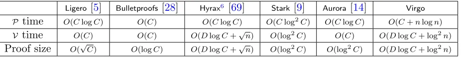
We present a new succinct zero knowledge argument scheme for layered arithmetic circuits without trusted setup. The prover time is O(C+nlogn) and the proof size is O(DlogC+ log2n) for a D-depth circuit withninputs andC gates. The verification time is also succinct, O(DlogC+ log2n), if the circuit is structured. Our scheme only uses lightweight cryptographic primitives such as collision-resistant hash functions and is plausibly post-quantum secure. We implement a zero knowledge argument system, Virgo, based on our new scheme and compare its performance to existing schemes. Experiments show that it only takes 53 seconds to generate a proof for a circuit computing a Merkle tree with 256 leaves, at least an order of magnitude faster than all other succinct zero knowledge argument schemes. The verification time is 50ms, and the proof size is 253KB, both competitive to existing systems.
Underlying Virgo is a new transparent zero knowledge verifiable polynomial delegation scheme with logarithmic proof size and verification time. The scheme is in the interactive oracle proof model and may be of independent interest.
1
Introduction
Zero knowledge proof (ZKP) allows a powerful prover to convince a weak verifier that a statement is true, without leaking any extra information about the statement beyond its validity. In recent years, significant progress has been made to bring ZKP protocols from purely theoretical interest to practical implementations, leading to its numerous applications in delegation of computations, anonymous credentials, privacy-preserving cryptocurrencies and smart contracts.
Despite of these great success, there are still some limitations of existing ZKP systems. In SNARK [60], the most commonly adopted ZKP protocol in practice, though the proof sizes are of just hundreds of bytes and the verification times are of several milliseconds regardless of the size of the statements, it requires a trusted setup phase to generate structured reference string (SRS) and the security will be broken if the trapdoor is leaked.
To address this problem, many ZKP protocols based on different techniques have been proposed recently to remove the trusted setup, which are referred astransparentZKP protocols. Among these techniques, ZKP schemes based on the doubly efficient interactive proof proposed by Goldwasser et al. in [42] (referred asGKR protocol in this paper) are particularly interesting due to their efficient prover time and sublinear verification time for statements represented as structured arithmetic
∗
to appear at IEEE Symposium on Security and Privacy 2020.
†
University of California, Berkeley. Email: {jiaheng_zhang,tianc.x,dawnsong}@berkeley.edu.
‡
Texas A&M University. Email: [email protected].
circuits, making it promising to scale to large statements. Unfortunately, as of today we are yet to construct an efficient transparent ZKP system based on the GKR protocol with succinct1 proof size
and verification time. The transparent scheme in [69] has square-root proof size and verification time, while the succinct scheme in [70] requires a one-time trusted setup. See Section1.2 for more details.
Our contributions. In this paper, we advance this line of research by proposing a transparent ZKP protocol based on GKR with succinct proof size and verification time, when the arithmetic circuit representing the statement is structured. The prover time of our scheme is particularly efficient, at least an order of magnitude faster than existing ZKP systems, and the verification time is merely tens of milliseconds. Our concrete contributions are:
• Transparent zero knowledge verifiable polynomial delegation. We propose a new zero knowledge verifiable polynomial delegation (zkVPD) scheme without trusted setup. Compared to existing pairing-based zkVPD schemes [59,72,73], our new scheme does not require a trap-door and linear-size public keys, and eliminates heavy cryptographic operations such as modular exponentiation and bilinear pairing. Our scheme may be of independent interest, as polynomial delegation/commitment has various applications in areas such as verifiable secret sharing [6], proof of retrievability [71] and other constructions of ZKP [55].
• Transparent zero knowledge argument. Following the framework proposed in [73], we combine our new zkVPD protocol with the GKR protocol efficiently to get a transparent ZKP scheme. Our scheme only uses light-weight cryptographic primitives such as collision-resistant hash functions and is plausibly post-quantum secure.
• Implementation and evaluation. We implement a ZKP system, Virgo, based on our new scheme. We develop optimizations such that our system can take arithmetic circuits on the field generated by Mersenne primes, the operations on which can be implemented efficiently using integer additions, multiplications and bit operations in C++. We plan to open source our system.
1.1 Our Techniques
Our main technical contribution in this paper is a new transparent zkVPD scheme withO(NlogN) prover time,O(log2N) proof size and verification time, where N is the size of the polynomial. We summarize the key ideas behind our construction. We first model the polynomial evaluation as the inner product between two vectors of sizeN: one defined by the coefficients of the polynomial and the other defined by the evaluation point computed on each monomial of the polynomial. The former is committed by the prover (or delegated to the prover after preprocessing in the case of delegation of computation), and the later is publicly known to both the verifier and the prover. We then develop a protocol that allows the prover to convince the verifier the correctness of the inner product between a committed vector and a public vector with proof sizeO(log2N), based on the univariate sumcheck protocol recently proposed by Ben-Sasson et al. in [14] (See Section 2.4). To ensure security, the verifier needs to access the two vectors at some locations randomly chosen by the verifier during the protocol. For the first vector, the prover opens it at these locations using standard commitment schemes such as Merkle hash tree. For the second vector, however,
it takes O(N) time for the verifier to compute its values at these locations locally. In order to improve the verification time, we observe that the second vector is defined by the evaluation point of size only ` for a`-variate polynomial, which is O(logN) if the polynomial is dense. Therefore, this computation can be viewed as a function that takes ` inputs, expands them to a vector of
N monomials and outputs some locations of the vector. It is a perfect case for the verifier to use the GKR protocol to delegate the computation to the prover and validate the output, instead of computing locally. With proper design of the GKR protocol, the verification time is reduced to
O(log2N) and the total prover time is O(NlogN). We then turn the basic protocol into zero knowledge using similar techniques proposed in [5, 14]. The detailed protocols are presented in Section3.
1.2 Related Work
Zero knowledge proof. Zero knowledge proof was introduced by Goldwasser et al. in [43] and generic constructions based on probabilistically checkable proofs (PCPs) were proposed in the sem-inal work of Kilian [51] and Micali [58] in the early days. In recent years there has been significant progress in efficient ZKP protocols and systems. Following earlier work of Ishai [48], Groth [45] and Lipmaa [53], Gennaro et al. [40] introduced quadratic arithmetic programs (QAPs), which leads to efficient implementations of SNARKs [12, 17,24, 35, 38, 60, 68]. The proof size and verification time of SNARK are constant, which is particularly useful for real-world applications such as cryp-tocurrencies [11] and smart contract [23,52]. However, SNARKs require a per-statement trusted setup, and incurs a high overhead in the prover running time and memory consumption, making it hard to scale to large statements. There has been great research for generating the SRS through multi-parity secure computations [13] and making the SRS universal and updatable [46,55].
Many recent works attempt to remove the trusted setup and construct transparent ZKP schemes. Based on “(MPC)-in-the-head” introduced in [31,41,49], Ames et al. [5] proposed a ZKP scheme called Ligero. It only uses symmetric key operations and the prover time is fast in practice, but the proof size is O(√C) and the verification time is quasi-linear to the size of the circuit. Later, it is categorized as interactive oracle proofs (IOPs), and in the same model Ben-Sasson et al. built
Stark [9], transparent ZKP in the RAM model of computation. Their verification time is only linear to the description of the RAM program, and succinct (logarithmic) in the time required for program execution. Recently, Ben-Sasson et al. [14] proposed Aurora, a new ZKP system in the IOP model with the proof size of O(log2C). Our new zkVPD and ZKP schemes fall in the IOP model.
In the seminal work of [42], Goldwasser et al. proposed an efficient interactive proof for layered arithmetic circuits, which was extended to an arugment system by Zhang et al. in [74] using a protocol for verifiable polynomial delegation. Later, Zhang et al. [75], Wahby et al. [69] and Xie et al. [70] made the argument system zero knowledge by Cramer and Damgard transformation [36] and random masking polynomials [32]. The scheme of [69], Hyrax, is transparent, yet the proof size and verification time are O(√n) where n is the input size of the circuit; the schemes of [72] and [70] are succinct for structured circuits, but require one-time trusted setup. The prover time of the GKR protocol is substantially improved in [34, 64, 67, 69, 75], and recently Xie et al. [70] proposed a variant withO(C) prover time for arbitrary circuits.
Verifiable polynomial delegation. Verifiable polynomial delegation (VPD) allows a verifier to delegate the computation of polynomial evaluations to a powerful prover, and validates the result in time that is constant or logarithmic to the size of the polynomial. Earlier works in the literature include [18, 39, 50]. Based on [50], Papamanthou et al. [59] propose a protocol for multivariate polynomials. Later in [73], Zhang et al. extend the scheme to an argument of knowledge using powers of exponent assumptions, allowing a prover to commit to a multivariate polynomial, and open to evaluations at points queried by the verifier. In [72], Zhang et al. further make the scheme zero knowledge. These schemes are based on bilinear maps and require a trusted setup phase that generates linear-size public keys with a trapdoor.
In a concurrent work, B¨unz et al. [26] propose another transparent polynomial commitment scheme without trusted setup. The scheme utilizes groups of unknown order and the techniques are different from our construction. The prover and verifier time are O(N) and O(logN) modulo exponentiation in the group and the proof size is O(logN) group elements. Concretely, the proof size is 10-20KB for a circuit with 220 gates when compiled to different ZKP systems [26, Section 6], and the prover time and the verification time are not reported. Comparing to our scheme, we expect the prover and verifier time in our scheme are faster, while our proof size is larger, which gives an interesting trade-off.
2
Preliminaries
We use λ to denote the security parameter, and negl(λ) to denote the negligible function in λ. “PPT” stands for probabilistic polynomial time. For a multivariate polynomial f, its ”variable-degree” is the maximum degree off in any of its variables. We often rely on polynomial arithmetic, which can be efficiently performed via fast Fourier tranforms and their inverses. In particular, polynomial evaluation and interpolation over a multiplicative coset of size n of a finite field can be performed in O(nlogn) field operations via the standard FFT protocol, which is based on the divide-and-conquer algorthim.
2.1 Interactive Proofs and Zero-knowledge Arguments
Interactive proofs. An interactive proof allows a proverP to convince a verifierV the validity of some statement through several rounds of interaction. We say that an interactive proof is public coin if V’s challenge in each round is independent of P’s messages in previous rounds. The proof system is interesting when the running time of V is less than the time of directly computing the functionf. We formalize interactive proofs in the following:
Definition 1. Let f be a Boolean function. A pair of interactive machineshP,Viis an interactive proof for f with soundness if the following holds:
• Completeness. For every x such that f(x) = 1 it holds that Pr[hP,Vi(x) =1] = 1.
• -Soundness. For any x with f(x)6= 1 and any P∗ it holds that Pr[hP∗,Vi=1]≤
of the statement validity, then the prover must know w. We use G to represent the generation phase of the public parameters pp. Formally, consider the definition below, where we assume R is known to P and V.
Definition 2. LetRbe an NP relation. A tuple of algorithm(G,P,V)is a zero-knowledge argument of knowledge for R if the following holds.
• Correctness. For everypp output by G(1λ) and (x, w)∈R,
hP(pp, w),V(pp)i(x) =1
• Soundness. For any PPT proverP, there exists a PPT extractorεsuch that for everyppoutput by G(1λ) and any x, the following probability is negl(λ):
Pr[hP(pp),V(pp)i(x) =1∧(x, w)∈ R|/ w←ε(pp, x)]
• Zero knowledge. There exists a PPT simulatorS such that for any PPT algorithmV∗, auxiliary input z∈ {0,1}∗, (x;w)∈ R, ppoutput by G(1λ), it holds that
View(hP(pp, w),V∗(z,pp)i(x))≈ SV∗(x, z)
We say that (G,P,V) is a succinct argument system if the running time of V and the total com-munication between P andV (proof size) are poly(λ,|x|,log|w|).
In the definition of zero knowledge,SV∗denotes that the simulatorSis given the randomness of V∗ sampled from polynomial-size space. This definition is commonly used in existing transparent zero knowledge proof schemes [5,14,28,69].
2.2 Zero-Knowledge Verifiable Polynomial Delegation
Let F be a finite field, F be a family of `-variate polynomial over F, and d be a variable-degree parameter. We use W`,d to denote the collection of all monomials in F and N =|W`,d|= (d+ 1)`. A zero-knowledge verifiable polynomial delegation scheme (zkVPD) for f ∈ F and t∈F` consists of the following algorithms:
• pp←zkVPD.KeyGen(1λ),
• com←zkVPD.Commit(f, rf,pp),
• ((y, π);{0,1})← hzkVPD.Open(f, rf),zkVPD.Verify(com)i(t,pp)
Note that unlike the zkVPD in [59, 72, 73], our definition is transparent and does not have a trapdoor in zkVPD.KeyGen. π denotes the transcript seen by the verifier during the interaction withzkVPD.Open, which is similar to the proof in non-interactive schemes in [59,72,73].
Definition 3. A zkVPD scheme satisfies the following properties:
• Completeness. For any polynomial f ∈ F and value t∈F`, pp←zkVPD.KeyGen(1λ), com ←
zkVPD.Commit(f, rfpp), it holds that
• Soundness. For any PPT adversary A, pp ← zkVPD.KeyGen(1λ), the following probability is negligible of λ:
Pr
(f∗,com∗, t)← A(1λ,pp)
((y∗, π∗);1)← hA(),zkVPD.Verify(com∗)i(t,pp)
com∗=zkVPD.Commit(f∗,pp)
f∗(t)6=y∗
• Zero Knowledge. For security parameterλ, polynomialf ∈ F,pp←zkVPD.KeyGen(1λ), PPT algorithm A, and simulatorS = (S1,S2), consider the following two experiments:
RealA,f(pp):
1. com←zkVPD.Commit(f, rf,pp)
2. t← A(com,pp)
3. (y, π)← hzkVPD.Open(f, rf),Ai(t,pp)
4. b← A(com, y, π,pp)
5. Output b
IdealA,SA(pp):
1. com← S1(1λ,pp)
2. t← A(com,pp)
3. (y, π)← hS2,Ai(ti,pp), given oracle access toy=f(t).
4. b← A(com, y, π,pp)
5. Output b
For any PPT algorithm A and all polynomial f ∈F, there exists simulatorS such that
|Pr[RealA,f(pp) = 1]−Pr[IdealA,SA(pp) = 1]| ≤negl(λ).
2.3 Zero Knowledge Argument Based on GKR
In [70], Xie et al. proposed an efficient zero knowledge argument scheme named Libra. The scheme extends the interactive proof protocol for layered arithmetic circuits proposed by Goldwasser et al. [42] (referred as the GKR protocol) to a zero knowledge argument using multiple instances of zkVPD schemes. Our scheme follows this framework and we review the detailed protocols here.
Sumcheck protocol. The sumcheck protocol is a fundamental protocol in the literature of inter-active proof that has various applications. The problem is to sum a polynomial f :F` →Fon the binary hypercubeP
b1,b2,...,b`∈{0,1}f(b1, b2, ..., b`).Directly computing the sum requires exponential
time in`, as there are 2` combinations ofb1, . . . , b`. Lund et al. [54] proposed asumcheck protocol that allows a verifier V to delegate the computation to a computationally unbounded prover P, who can convince V the correctness of the sum. At the end of the sumcheck protocol,V needs an oracle access to the evaluation of f at a random point r ∈F` chosen by V. The proof size of the sumcheck protocol is O(d`), where d is the variable-degree of f, and the verification time of the protocol is O(d`). The sumcheck protocol is complete and sound with= |d`
F|.
Formally speaking, we denote the number of gates in the i-th layer asSi and let si=dlogSie. We then define a function Vi :{0,1}si →F that takes a binary stringb∈ {0,1}si and returns the output of gate b in layer i, where b is called the gate label. With this definition, V0 corresponds to the output of the circuit, andVD corresponds to the input. As the sumcheck protocol works on F, we then extend Vi to its multilinear extension, the unique polynomial ˜Vi :Fsi → F such that
˜
Vi(x1, x2, ..., xsi) =Vi(x1, x2, ..., xsi) for all x1, x2, . . . , xsi ∈ {0,1}
si. As shown in prior work [34],
the closed form of ˜Vi can be computed as:
˜
Vi(x1, x2, ..., xsi) =
X
b∈{0,1}si
si
Y
i=1
[((1−xi)(1−bi) +xibi)·Vi(b)], (1)
wherebi isi-th bit of b.
With these definitions, we can express the evaluations of ˜Vi as a summation of evaluations of ˜
Vi+1:
αiV˜i(u(i)) +βiV˜i(v(i)) =
X
x,y∈{0,1}si+1fi( ˜Vi+1(x),
˜
Vi+1(y)), (2)
where u(i), v(i) ∈ Fsi are random vectors and α
i, βi ∈ F are random values. Note here that fi depends onαi, βi, u(i), v(i) and we omit the subscripts for easy interpretation.
With Equation2, the GKR protocol proceeds as follows. The proverP first sends the claimed output of the circuit to V. From the claimed output, V defines polynomial ˜V0 and computes
˜
V0(u(0)) and ˜V0(v(0)) for random u(0), v(0) ∈ Fs0. V then picks two random values α0, β0 and invokes a sumcheck protocol on Equation2withP fori= 0. As described before, at the end of the sumcheck,V needs an oracle access to the evaluation off0 atu(1), v(1) randomly selected inFs1. To compute this value, V asks P to send ˜V1(u(1)) and ˜V1(v(1)). Other than these two values, f0 only depends onα0, β0, u(0), v(0) and the gates and wiring in layer 0, which are all known to V and can be computed byV directly. In this way,V and P reduces two evaluations of ˜V0 to two evaluations of ˜V1in layer 1. V andP then repeat the protocol recursively layer by layer. Eventually,V receives two claimed evaluations ˜VD(u(D)) and ˜VD(v(D)). V then checks the correctness of these two claims directly by evaluating ˜VD, which is defined by the input of the circuit. LetGKR.P and GKR.V be the algorithms for the GKR prover and verifier, we have the following theorem:
Lemma 1. [34, 42, 64, 70]. Let C : Fn → F be a layered arithmetic circuit with depth of D. hGKR.P,GKR.Vi(C, x) is an interactive proof per Definition 1 for the function computed by C on inputxwith soundness O(Dlog|C|/|F|). The total communication isO(Dlog|C|) and the running
time of the proverP isO(|C|). WhenC has regular wiring pattern2, the running time of the verifier
V is O(n+Dlog|C|).
Extending GKR to Zero Knowledge Argument. There are two limitations of the GKR protocol: (1) It is not an argument system supporting witness fromP, as V needs to evaluate ˜VD locally in the last round; (2) It is not zero knowledge, as in each round, both the sumcheck protocol and the two evaluations of ˜Vi leak information about the values in layeri.
To extend the GKR protocol to a zero knowledge argument, Xie et al. [70] address both of the problems using zero knowledge polynomial delegation. Following the approach of [69, 72, 73], to
2“Regular” circuits is defined in [34, Theorem A.1]. Roughly speaking, it means the mutilinear extension of its
Protocol 1 (Zero Knowledge Argument in [70]). Let λ be the security parameter, F be a prime field. Let C : Fn
→ F be a layered arithmetic circuit over F with D layers, input in and witness w such that
|in|+|w| ≤n and1 =C(in;w).
• G(1λ): set pp aspp←zkVPD.KeyGen(1λ).
• hP(pp, w),V(pp)i(in):
1. P selects a random bivariate polynomialRD. P commits to the witness of C by sending comD←
zkVPD.Commit( ˙VD, rVD,pp)toV, whereV˙D is defined by Equation 3.
2. P randomly selects polynomials Ri : F2 → F and δi : F2si+1+1 →
F for i = 0, . . . , D−1.
P commits to these polynomials by sending comi,1 ← zkVPD.Commit(Ri, rRi,pp) and comi,2 ←
zkVPD.Commit(δi, rδi,pp)toV. P also revealsR0 toV, asV0 is known toV.
3. V evaluates V˙0(u(0)) andV˙0(v(0))for randomly chosenu(0), v(0)∈Fs0.
4. For i= 0, . . . , D−1:
(a) P sends Hi=Px,y∈{0,1}si+1,z∈{0,1}δi(x, y, z)toV.
(b) V picksαi, βi, γi randomly in F.
(c) V andP execute a sumcheck protocol on Equation4. At the end of the sumcheck,V receives a claim offi0 at point u(i+1), v(i+1)
∈Fsi+1, gi∈Fselected randomly by V.
(d) P opensRi(u(i), gi),Ri(v(i), gi)andδi(u(i+1), v(i+1), gi)usingzkVPD.Open. P sendsV˙0(u(i+1))
andV˙0(v(i+1))toV.
(e) V validatesRi(u(i), gi),Ri(v(i), gi)andδi(u(i+1), v(i+1), gi)usingzkVPD.Verify. If any of them
outputs 0, abort and output0.
(f ) V checks the claim of fi0 using Ri(u(i), gi), Ri(v(i), gi), δi(u(i+1), v(i+1), gi), V˙0(u(i+1)) and ˙
V0(v(i+1)). If it fails, output0.
5. P runs (y1, π1) ← zkVPD.Open( ˙VD, rVD, u
(D),pp), (y
2, π2)← zkVPD.Open( ˙VD, rVD, v
(D),pp) and
sendsy1, π1, y2, π2 toV.
6. V runsVerify(π1, y1,comD, u(D),pp)and Verify(π2, y2,comD, v(D),pp) and output0 if either check
fails. Otherwise,VchecksV˙D(u(D)) =y1andV˙D(v(D)) =y2, and rejects if either fails. If all checks
above pass,V output1.
support witness w as the input to the circuit, P commits to ˜VD using zkVPD before running the GKR protocol. In the last round of GKR, instead of evaluating ˜VD locally,V asksP to open ˜VD at two random pointsu(D), v(D) selected by V and validates them usingzkVPD.Verify. In this way, V does not need to accesswdirectly and the soundness still holds because of the soundness guarantee of zkVPD.
To ensure zero knowledge, using the techniques proposed by Chiesa et al. in [32], the prover P masks the polynomial ˜Vi and the sumcheck protocol by random polynomials so that the proof does not leak information. For correctness and soundness purposes, these random polynomials are committed using the zkVPD protocol and opened at random points chosen byV. In particular, for layer i, the prover selects a random bivariate polynomial Ri(x1, z) and defines
˙
Vi(x1, . . . , xsi)
def
= ˜Vi(x1, . . . , xsi) +Zi(x1, . . . , xsi)
X
z∈{0,1}
Ri(x1, z), (3)
where Zi(x) = Qis=1i xi(1−xi), i.e., Zi(x) = 0 for all x ∈ {0,1}si. ˙Vi is known as the low degree
P, revealing evaluations of ˙Vi does not leak information about Vi, thus the values in the circuit. Additionally, P selects another random polynomial δi(x1, . . . , xsi+1, y1, . . . , ysi+1, z) to mask the
sumcheck protocol. Let Hi = Px,y∈{0,1}si+1,z∈{0,1}δi(x1, . . . , xsi+1, y1, . . . , ysi+1, z), Equation 2 to
run sumcheck on becomes
αiV˙i(u(i)) +βiV˙i(v(i)) +γiHi
=X
x,y∈{0,1}si+1,z∈{0,1}f
0
i( ˙Vi+1(x),V˙i+1(y), Ri(u1(i), z), Ri(v1(i), z), δi(x, y, z)), (4)
where γi ∈ F is randomly selected by V, and fi0 is defined by αi, βi, γi, u(i), v(i), Zi(u(i)), Zi(v(i))3. Now V and P can execute the sumcheck and GKR protocol on Equation 4. In each round, P additionally opensRi andδi atRi(u1(i), g(i)), Ri(v(1i), g(i)), δi(u(i+1), v(i+1), g(i)) forg(i) ∈Frandomly selected byV. With these values,V reduces the correctness of two evaluations ˙Vi(u(i)),V˙i(v(i)) to two evaluations ˙Vi(u(i+1)),V˙i(v(i+1)) on one layer above like before. In addition, asfi is masked by
δi, the sumcheck protocol is zero knowledge; as ˜Vi is masked by Ri, the two evaluations of ˙Vi do not leak information. The full zero knowledge argument protocol in [70] is given in Protocol1. We have the following theorem:
Lemma 2. [70]. LetC: Fn→Fbe a layered arithmetic circuit withDlayers, inputinand witness
w. Protocol1 is a zero knowledge argument of knowledge under Definition2 for the relation defined by 1 =C(in;w).
The variable degree ofRi isO(1). δi(x, y, z) =δi,1(x1) +. . .+δi,si+1(xsi+1) +δi,si+1+1(y1) +. . .+ δi,2si+1(ysi+1) +δi,2si+1+1(z) is the summation of 2si+1+ 1 univariate polynomials of degree O(1). Other than the zkVPD instantiations, the proof size is O(Dlog|C|) and the prover time isO(|C|). When C is regular, the verification time is O(n+Dlog|C|).
2.4 Univariate Sumcheck
Our transparent zkVPD protocol is inspired by the univariate sumcheck protocol recently proposed by Ben-Sasson et al.in [14]. As the name indicates, the univariate sumcheck protocol allows the verifier to validate the result of the sum of a univariate polynomial on a subset H of the field F:
µ=P
a∈Hf(a). The key idea of the protocol relies on the following lemma:
Lemma 3. [27]. Let H be a multiplicative coset4 of F, and let g(x) be a univariate polynomial
over F of degree strictly less that |H|. Then Pa∈Hg(a) =g(0)· |H|.
Because of Lemma 3, to test the result of P
a∈Hf(a) for f with degree less than k, we can decomposef into two partsf(x) =g(x) +ZH(x)·h(x), whereZH(x) =Q
a∈H(x−a) (i.e.,ZH(a) = 0
for alla∈H), and the degrees ofgand hare strictly less than|H|andk− |H|. This decomposition is unique for every f. AsZH(a) is always 0 fora∈H,µ=Pa∈Hf(a) =
P
a∈Hg(a) =g(0)· |H|by
Lemma3. Therefore, if the claimed sumµsent by the prover is correct,f(x)−ZH(x)·h(x)−µ/|H| must be a polynomial of degree less than|H|with constant term 0, or equivalently polynomial
p(x) = |H| ·f(x)− |H| ·ZH(x)·h(x)−µ
|H| ·x (5)
3
Formally, fi0 is I(0, z)fi( ˙Vi+1(x),V˙i+1(y)) +I((x, y),0)(αiZi(u(i))R(u1(i), z) +βiZi(v(i))R(v1(i), z)) +γiδi(x, y, z), whereI(a, b) is an identity polynomialI(a, b) = 0 iffa=b. We will not usefi0 explicitly in our constructions later.
4In [14], the protocols are mainly using additive cosets. We require
H to be a multiplicative coset for our
must be a polynomial of degree less than|H| −1. To test this, the univariate sumcheck uses a low degree test (LDT) protocol on Reed-Solomon (RS) code, which we define below.
Reed-Solomon Code. LetLbe a subset ofF, an RS code is the evaluations of a polynomialρ(x) of degree less thanm(m <L) onL. We use the notationρ|Lto denote the vector of the evaluations
(ρ(a))a∈L, and useRS[L, m] to denote the set of all such vectors generated by polynomials of degree
less thanm. Note that any vector of size|L|can be viewed as some univariate polynomial of degree less than|L|evaluated on L, thus we use vector and polynomial interchangeably.
Low Degree Test and Rational Constraints. Low degree test allows a verifier to test whether a polynomial/vector belongs to an RS code, i.e., the vector is the evaluations of some polynomial of degree less than m on L.
In our constructions, we use the LDT protocol in [14, Protocol 8.2], which was used to transform an RS-encoded IOP to a regular IOP. It applies the LDT protocol proposed in [10] protocol to a sequence of polynomials ~ρ and their rational constraint p, which is a polynomial that can be computed as the division of the polynomials in~ρ. In the case of univariate sumcheck, the sequence of polynomials is~ρ= (f, h) and the rational constraint is given by Equation 5.
The high level idea is as follows. First, the verifier multiplies each polynomial in ~ρ and the rational constraintp with an appropriate monomial such that they have the same degreemax, and takes their random linear combination. Then the verifier tests that the resulting polynomial is in
RS[L,max+ 1]. At the end of the protocol, the verifier needs oracle access toκ evaluations of each polynomial in ρ~ and the rational constraint p at points in L indexed by I, and checks that each evaluation of pis consistent with the evaluations of the polynomials in ~ρ. We denote the protocol ashLDT.P(ρ, p~ ),LDT.V(m,~ deg(p))i(L), where ~ρ is a sequence of polynomials over F,p(x) is their rational constraint,m,~ deg(p) is the degrees of the polynomials and the rational constraint to test, andLis a multiplicative coset ofF. We state the properties of the protocol in the following lemma:
Lemma 4. There exist an LDT protocol hLDT.P(~ρ, p),LDT.V(m,~ deg(p))i(L) that is complete and
sound with soundness errorO(|L|
|F|) +negl(κ), given oracle access to evaluations of each polynomial
in ~ρ at κ points indexed by I in L. The proof size and the verification time are O(log|L|) other
than the oracle access, and the prover time is O(L).
The LDT protocol can be made zero knowledge in a straight-forward way by adding a ran-dom polynomial of degree max in ~ρ. That is, there exists a simulator S such that given the random challenges of I of any PPT algorithm V∗, it can simulate the view of V∗ such that
View(hLDT.P(~ρ, p),V∗(m,~ deg(p))i(
L))≈ SV ∗
(deg(p)). In particular,Sgeneratesp∗ ∈RS[L,deg(p)] and can simulate the view of any sequence of random polynomialsρ~∗ subject to the constraint that their evaluations at points indexed by I are consistent with the oracle access ofp∗.
Merkle Tree. Merkle hash tree proposed by Ralph Merkle in [57] is a common primitive to commit a vector and open it at an index with logarithmic proof size and verification time. It consists of three algorithms:
• rootc←MT.Commit(c)
• (cidx, πidx)←MT.Open(idx, c)
The security follows the collision-resistant property of the hash function used to construct the Merkle tree.
With these tools, the univariate sumcheck protocol works as follows. To proveµ=P
a∈Hf(a),
the verifier and the prover picks L, a multiplicative coset of F and a superset of H, where |L|>
k. P decompose f(x) = g(x) +ZH(x) ·h(x) as defined above, and computes the vectors f|L
and h|L. P then commits to these two vectors using Merkle trees. P then defines a polynomial p(x) = |H|·f(x)−|H|·ZH(x)·h(x)−µ
|H|·x , which is a rational constraint of f and h. As explained above,
in order to ensure the correctness of µ, it suffices to test that the degree of (f, h), p is less than (k, k− |H|),|H| −1, which is done through the low degree test. At the end of the LDT,V needs oracle access to κ points of f|L and h|L. P sends these points with their Merkle tree proofs, and
V validates their correctness. The formal protocol and the lemma is presented in AppendixA. As shown in [14], it suffices to set|L|=O(|H|).
3
Transparent Zero Knowledge Polynomial Delegation
In this section, we present our main construction, a zero knowledge verifiable polynomial delegation scheme without trusted setup. We first construct a VPD scheme that is correct and sound, then extend it to be zero knowledge. Our construction is inspired by the univariate sumcheck [14] described in Section 2.4.
Our main idea is as follows. To evaluate an `-variate polynomial f with variable degree d
at point t = (t1, . . . , t`), we model the evaluation as the inner product between the vector of coefficients in f and the vector of all monomials in f evaluated at t. Formally speaking, let
N = |W`,d| = (d+ 1)` be the number of possible monomials in an `-variate polynomial with variable degreed, and letc= (c1, . . . , cN) be the coefficients off in the order defined byW`,d such that f(x1, . . . , x`) = PNi=1ciWi(x), where Wi(x) is the i-th monomial in W`,d. Define the vector
T = (W1(t), . . . , WN(t)), then naturally the evaluation equalsf(t) =PNi=1ci·Ti, the inner product of the two vectors. We then select a multiplicative coset H such that|H|=N, 5 and interpolate vectors c and T to find the unique univariate polynomials that evaluate to c and T on H. We denote the polynomials as l(x) and q(x) such that l|H = c and q|H = T. With these definitions,
f(t) = PN
i=1ci ·Ti = Pa∈Hl(a)·q(a), which is the sum of the polynomial l(x)·q(x) on H. The
verifier can check the evaluation through a univariate sumcheck protocol with the prover. The detailed protocol is presented in step 1-4 of Protocol 2.
Up to this point, the construction for validating the inner product between a vector committed by P and a public vector is similar to and simpler than the protocols to check linear constraints proposed in [5, 14]. However, naively applying the univariate sumcheck protocol incurs a linear overhead for the verifier. This is because as described in Section 2.4, at the end of the univariate sumcheck, due to the low degree test, the verifier needs oracle access to the evaluations ofl(x)·q(x) atκ points onL, a superset of H. Asl(x) is defined by c, i.e. the coefficients of f, the prover can commit to l|L at the beginning of the protocol, and opens to points the verifier queries with their Merkle tree proofs. q(x), however, is defined by the public vectorT, and the verifier has to evaluate it locally, which takes linear time. This is the major reason why the verification time in the zero knowledge proof schemes for generic arithmetic circuits in [5,14] is linear in the size of the circuits.
5
If such coset does not exist, we can pad N to the nearest number with a coset of that size, and pad vector T
Protocol 2 (Verifiable Polynomial Delegation). Let F be a family of `-variate polynomial over F with variable-degree d and N = (d+ 1)`.We use
W`,d = {Wi(x1, . . . , x`)}Ni=1 to denote the collection of all
monomials inF. rf =⊥and we omit if in the algorithms.
• pp←KeyGen(1λ): Pick a hash function from the collision-resistant hash function family for Merkle tree.
Find a multiplicative cosetHofF such that |H|= (d+ 1)`. Find a multiplicative coset
L ofF such that
|L|=O(|H|)>2|H| andH⊂L⊂F.
• com ← Commit(f,pp): For a polynomial f ∈ F of the form f(x) = PNi=1ciWi(x), find the unique
univariate polynomial l(x) : F → F such that l|H = (c1, . . . , cN). P evaluates l|L and runs rootl ←
MT.Commit(l|L). Outputcom=rootl.
• ((µ, π);{0,1})← hOpen(f),Verify(com)i(t,pp): This is an interactive protocol betweenP andV.
1. P computesµ=f(t)and sends it toV.
2. P evaluatesT = (W1(t), . . . , WN(t)). P finds the unique univariate polynomial q(x) :F→Fsuch
thatq|H=T.
3. P computes l(x)·q(x). P uniquely decomposes l(x)·q(x) =g(x) +ZH(x)·h(x) , where ZH(x) = Q
a∈H(x−a)and the degrees of gandhare strictly less than|H| and|H| −1. P evaluatesh|L and
runsrooth←MT.Commit(h|L)and sends rooth toV.
4. Let p(x) = |H|·l(x)·q(x)−µ−|H|·ZH(x)h(x)
|H|·x . P and V invoke a low degree test: hLDT.P((l ·
q, h), p),LDT.V((2|H| −1,|H| −1),|H| −1)i(L). If the test fails, V aborts and output 0. Other-wise, at then end of the test,V needs oracle access toκpoints ofl(x)·q(x), h(x)andp(x)at indices
I.
5. For each index i∈ I, letai be the corresponding point inL. P opens(l(ai), πli)←MT.Open(i, l|L)
and(h(ai), πhi)←MT.Open(i, h|L).
6. V executesMT.Verify(rootl, i, l(ai), πil)andMT.Verify(rooth, i, h(ai), πih)for all points opened by P.
If any verification fails, abort and output0.
7. To complete the low degree test,P andV runshGKR.P,GKR.Vi(C, t), where circuitCcomputes the evaluations of q|L and outputs the elementsq(ai)for i∈ I (see Figure 1). If any of the checks in
GKR fails,V aborts and outputs 0.
8. For eachi∈ I,V computesl(ai)·q(ai). Together withh(ai),V completes the low degree test. If all
checks above pass,V outputs 1.
Reducing the verification time. In this paper, we propose an approach to reduce the cost of the verifier to poly-logarithmic for VPD. We observe that in our construction, though the size of
T and q(x) is linear inN, it is defined by only`=O(logN) values of the evaluation pointt. This means that the oracle access ofκ points of q(x) can be modeled as a function that: (1) Takestas input, evaluates all monomials Wi(t) for all Wi ∈ W`,d as a vector T; (2) Extrapolates the vector
T to find polynomial q(x), and evaluates q(x) on L; (3) Outputs κ points of q|L chosen by the
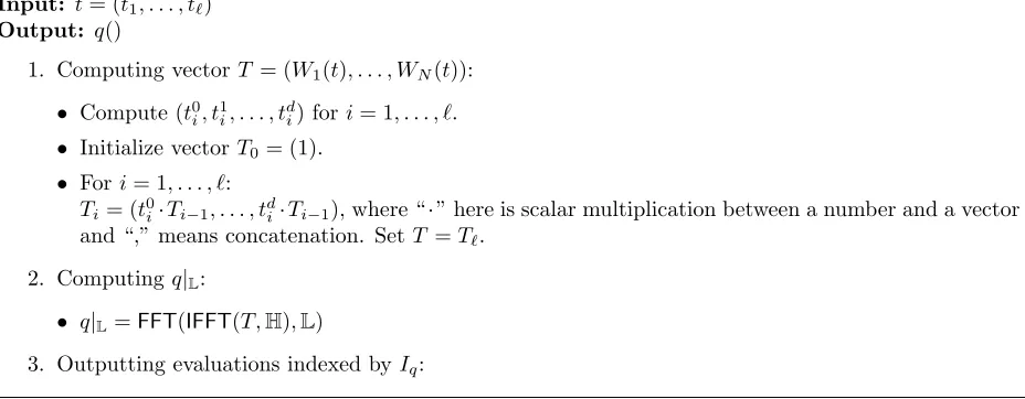
verifier. Although the size of the function modeled as an arithmetic circuit is Ω(N) with O(logN) depth, and the size of its input and output is onlyO(logN+κ). Therefore, instead of evaluating the function locally, the verifier can delegate this computation to the prover, and validate the result using the GKR protocol, as presented in Section 2.3. In this way, we eliminate the linear overhead to evaluate these points locally, making the verification time of the overall VPD protocol poly-logarithmic. The formal protocol is presented in Protocol2.
Input: t= (t1, . . . , t`) Output: q()
1. Computing vectorT = (W1(t), . . . , WN(t)):
• Compute (t0
i, t1i, . . . , tdi) fori= 1, . . . , `. • Initialize vectorT0= (1).
• Fori= 1, . . . , `:
Ti = (t0i·Ti−1, . . . , tdi·Ti−1), where “·” here is scalar multiplication between a number and a vector and “,” means concatenation. SetT =T`.
2. Computingq|L:
• q|L=FFT(IFFT(T,H),L)
3. Outputting evaluations indexed by Iq:
Figure 1: Arithmetic circuit C computing evaluations of q(x) at κ points inL indexed byI.
circuit for the function mentioned above. The details of the circuit are presented in Figure 1. In particular, in the first part, each valueti in the inputtis raised to powers of 0,1, . . . , d. Then they are expanded toT, the evaluations of all monomials inW`,d, by multiplying onetiat a time through a (d+ 1)-ary tree. The size of this part isO(N) =O((d+ 1)`) and the depth isO(logd+`). In the second part, the polynomial q(x) and the vectorq|L is computed from T directly using FFTs. We
first construct a circuit for an inverse FFT to compute the coefficients of polynomial q(x) from its evaluations T. Then we run an FFT to evaluate q|L from the coefficients of q(x). We implement FFT and IFFT using the Butterfly circuit [33]. The size of the circuit isO(NlogN) and the depth isO(logN). Finally,κ points are selected fromq|L. As the whole delegation of the GKR protocol
is executed at the end in Protocol 2 after these points being fixed by the verifier, the points to output are directly hard-coded into the circuit with size O(κ) and depth 1. No heavy techniques for random accesses in the circuit is needed. Therefore, the whole circuit is of sizeO(NlogN) and depthO(logN), with `inputs and κ outputs.
Theorem 1. Protocol 2 is a verifiable polynomial delegation protocol that is complete and sound under Definition 3.
Proof. Completeness. By the definition of l(x) and q(x), ifµ=f(t), thenµ=P
a∈Hl(a)·q(a) =
P
a∈Hg(a) = g(0)· |H|by Lemma 3. Thus, p(x) =
|H|·l(x)·q(x)−|H|·ZH(x)h(x)−µ
|H|·x =
g(x)−g(0)
x , which is inRS[L,|H| −1]. The rest follows the completeness of the LDT protocol and the GKR protocol.
Soundness. LetεLDT, εMT, εGKRbe the soundness error of the LDT, Merkle tree and GKR proto-cols. There are two cases for a malicious proverP.
Case 1:@l∗∈RS[L,|H|+ 1] such thatcom=MT.Commit(l∗|L), i.e. comis not a valid commitment.
• By the check in step 6, if com is not a valid Merkle tree root, the verification passes with probability less thanεMT.
• If ∃l∗∗ ∈/ RS[L,|H|+ 1] such that com ← MT.Commit(l∗∗|L), if the points v
∗
i opened by P in step 5 v∗i 6=l∗∗(ai) for some i, the verification passes with probability no more thanεMT. • If the output qi∗ returned by P in step 7 is qi∗ 6= q(ai) for some i, the verification passes with
• Otherwise, as l∗∗(x)·q(x) ∈/ RS[L,2|H|+ 1], by the checks of LDT in step 4, the verification passes with probability no more than εLDT.
Case 2: ∃l∗ ∈ RS[L,|H|+ 1] such that com = MT.Commit(l∗|L). Let c
∗ = l∗|
H and f
∗(x) =
PN
i=1c
∗
iWi(x), then com = Commit(f∗,pp). Suppose µ∗ 6= f∗(t), then µ∗ 6=
P
a∈Hl∗(a)q(a).
Then by Lemma 3, for all h ∈ RS[L,|H|+ 1], p∗ ∈/ RS[L,|H| − 1], as Pa∈H(p
∗(a) ·a) =
P
a∈H
|H|·l∗(a)·q(a)−µ∗
|H| =
P
a∈H(l
∗(a)·q(a))−µ∗6= 0. Therefore,
• Similar to case 1, if the commitment in step 3 is not a valid Merkle tree root, or the points opened by P in step 5 are inconsistent with h or l∗, the verification passes with probability no more than εMT.
• If the output q∗i returned by P in step 7 qi∗ 6= q(ai) for some i, the verification passes with probability no more than εGKR.
• Otherwise, as l∗·q∈RS[L,2|H|+ 1], eitherh /∈RS[L,|H|+ 1] orp /∈RS[L,|H| −1] as explained above. By the check in step 4, the verification passes with probability no more than εLDT.
By the union bound, the probability of the event of a malicious prover is no more thanO(εLDT+
εMT+εGKR). As stated in Section2,εLDT=O(||LF||) +negl(κ),εGKR=O(log
2N
|F| ) andεMT=negl(λ). Therefore, with proper choice of parameters, the probability is≤negl(λ).
Efficiency. The running time ofCommit isO(NlogN). C in step 7 is a regular circuit with size
O(NlogN), depth O(`+ logd) and size of input and output O(`+κ). By Lemma 1 and 5, the prover time isO(NlogN), the proof size and the verification time are (log2N).
Extending to other ZKP schemes. We notice that our technique can be potentially applied to generic zero knowledge proof schemes in [5, 14] to improve the verification time for circuits/con-straint systems with succinct representation. As mentioned previously, the key step that introduces linear verification time in these schemes is to check a linear constraint system, i.e., y=Aw, where
w is a vector of all values on the wires of the circuit committed by the prover, and A is a public matrix derived from the circuit such thatAwgives a vector of left inputs to all multiplication gates in the circuit. (This check is executed 2 more times to also give right inputs and outputs.) To check the relationship, it is turned into a vector inner productµ=ry=rA·wby multiplying both sides by a random vector r. Similar to our naive protocol to check inner product, the verification time is linear in order to evaluate the polynomial defined by rA atκ points. With our new protocol, if the circuit can be represented succinctly in sublinear or logarithmic space, A can be computed by a function with sublinear or logarithmic number of inputs. We can use the GKR protocol to delegate the computation ofrAand the subsequent evaluations to the prover in a similar way as in our construction, and the verification time will only depend on the space to represent the circuit, but not on the total size of the circuit. This is left as a future work.
3.1 Achieving Zero Knowledge
Our VPD protocol in Protocol 2 is not zero knowledge. Intuitively, there are two places that leak information about the polynomial f: (1) In step 6 of Protocol 2, P opens evaluations of
Protocol 3(Zero Knowledge Verifiable Polynomial Delegation). LetF be a family of`-variate polynomial overFwith variable-degreedandN= (d+ 1)`.We use
W`,d={Wi(x1, . . . , x`)}Ni=1 to denote the collection
of all monomials inF.
• pp←zkVPD.KeyGen(1λ): Same asKeyGenin Procotol 2. Define
U=L−H.
• com ←Commit(f, rf,pp): For a polynomial f ∈ F of the form f(x) = PNi=1ciWi(x), find the unique
univariate polynomiall(x) :F→Fsuch thatl|H= (c1, . . . , cN). P samples a polynomialr(x)with degree
κrandomly and setsl0(x) =l(x) +ZH(x)·r(x), whereZH(x) =Q
a∈H(x−a). P evaluates l 0
|Uand runs
rootl0 ←MT.Commit(l0|U). Outputcom=rootl0.
• ((µ, π);{0,1})← hOpen(f, rf),Verify(com)i(t,pp): This is an interactive protocol between P and V. It
replaces the univariate sumscheck onl(x)·q(x)byl0(x)·q(x) +αs(x)andLby Uin Protocol2.
1. P computesµ=f(t)and sends it toV.
2. P evaluatesT = (W1(t), . . . , WN(t)). P finds the unique univariate polynomial q(x) :F→Fsuch
thatq|H=T.
3. P samples randomly a degree2|H|+κ−1 polynomials(x). P sendsV S=Pa∈Hs(a)androots←
MT.Commit(s|U).
4. V picks α∈Frandomly and sends it to P.
5. P computesαl0(x)·q(x) +s(x). P uniquely decomposes it asg(x) +ZH(x)·h(x), where the degrees of
gandhare strictly less than|H|and|H|+κ. P evaluatesh|Uand sends rooth←MT.Commit((h|U)
toV.
6. Letp(x) = |H|·(αl0(x)·q(x)+s(x))−(αµ+S)−|H|·ZH(x)h(x)
|H|·x . P andV invoke the low degree test: hLDT.P((l
0
· q, h, s), p),LDT.V((2|H|+κ,|H|+κ,2|H|+κ),|H| −1)i(U). If the test fails, V aborts and output
0. Otherwise, at the end of the test,V needs oracle access to κpoints ofl0(x)·q(x), h(x), s(x)and
p(x)at indicesI.
7. For each indexi∈ I, letaibe the corresponding point inU. P opens(l0(ai), πl
0
i)←MT.Open(i, l0|U),
(h(ai), πhi)←MT.Open(i, h|U)and(s(ai), πis)←MT.Open(i, s|U).
8. V executes MT.Verify(rootl0, i, l0(ai), πl 0
i), MT.Verify(rooth, i, h(ai), πih) and
MT.Verify(roots, i, s(ai), πsi) for all points opened by P. If any verification fails, abort and
output0.
9. To complete the low degree test,P andV runshGKR.P,GKR.Vi(C, t), where circuitCcomputes the evaluations ofq|U and outputs the elements q(ai) fori∈ I. If any of the checks in GKR fails, V
aborts and outputs 0.
10. For eachi∈ I,V computesl0(ai)·q(ai). Together withh(ai)ands(ai),V completes the low degree
test. If all checks above pass,V outputs 1.
(l(x)·q(x), h(x)), p(x) and the proofs of LDT reveal information about the polynomials, which are related to f.
To make the protocol zero knowledge, we take the standard approaches proposed in [5,14]. To eliminate the former leakage of queries onl(x), the prover picks a random degreeκpolynomialr(x) and masks it asl0(x) =l(x) +ZH(x)·r(x), where as before, ZH(x) =Q
a∈H(x−a). Note here that
l0(a) =l(a) fora∈H, yet anyκevaluations ofl0(x) outside Hdo not reveal any information about
l(x) because of the masking polynomialr(x). The degree ofl0(x) is |H|+κ, and we denote domain U=L−H.
l0(x)·q(x), sendsS =P
a∈Hs(a) to V and runs the univariate sumcheck protocol on their random linear combination: αµ+S =P
a∈H(αl
0(x)·q(x) +s(x)) for a random α ∈
F chosen by V. This ensures that bothµ and S are correctly computed because of the random linear combination and the linearity of the univariate sumcheck, while leaking no information about l0(x)·q(x) during the protocol, as it is masked by s(x).
One advantage of our construction is that the GKR protocol used to compute evaluations of
q(x) in step 7 of Protocol 2 remains unchanged in the zero knowledge version of the VPD. This is because q(x) and its evaluations are independent of the polynomial f or any prover’s secret input. Therefore, it suffices to apply the plain version of GKR without zero knowledge, avoiding any expensive cryptographic primitives.
The full protocol for our zkVPD is presented in Protocol 3. Note that all the evaluations are on U=L−Hinstead of L, as evaluations on Hleaks information about the original l(x). s(x) is also committed and opened using Merkle tree for the purpose of correctness and soundness. The efficiency of our zkVPD protocol is asymptotically the same as our VPD protocol in Protocol 2, and the concrete overhead in practice is also small. We have the following theorem:
Theorem 2. Protocol3is a zero knowledge verifiable polynomial delegation scheme by Definition3.
Proof. Completeness. It follows the completeness of Protocol2.
Soundness. It follows the soundness of Protocol2 and the random linear combination. In partic-ular, in Case 2 of the proof of Theorem 1, if ∃l0∗ ∈ RS[L,|H|+κ+ 1], it can always be uniquely decomposed as l∗(x) =l0∗(x)−ZH(x)r∗(x) such that P
a∈Hl
0∗(a) =P
a∈Hl
∗(a) and the degree of
l∗(x) is |H|and the degree of r(x) is κ. If µ∗ =6 µ=Pa∈H(l∗(a)·q(a)) =
P
a∈H(l0∗(a)·q(a)), let
S∗ = P
a∈Hs∗(a) where s∗(x) is committed by P in step 5, then
P
a∈H(αl0∗(a)·q(a) +s∗(a)) =
αµ∗+S∗ =αµ+Sif and only ifα= Sµ∗−−Sµ∗, which happens with probability 1/|F|. The probability of other cases are the same as the proof of Theorem 1, and we omit the details here.
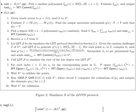
Zero knowledge. The simulator is given in Figure2.
To prove zero knowledge, lsim0 inS1 and l0 inzkVPD.Commitare both uniformly distributed. In S2, steps 1, 2 and 9 are the same as the real world in Protocol 3. No message is sent in steps 4, 8 and 10.
In step 3 and 7,ssim and sare both randomly selected and their commitments and evaluations are indistinguishable. As r(x) is a degree-κ random polynomial in the real world in Protocol3, κ
evaluations of l0(x) opened in step 7 are independent and randomly distributed, which is indistin-guishable from step 7 of S2 in the ideal world. Finally, in step 7 of the ideal world, V∗ receives κ evaluations of hsim at point indexed by I. Together with lsim0 ·q and ssim, by Lemma 4, the view of steps 5-7 simulated by LDT.S is indistinguishable from the real world withh, l0·q and s, which completes the proof.
Our zkVPD protocol is also a proof of knowledge. Here we give the formal definition of knowl-edge soundness of a zkVPD protocol in addition to Definition 3 and prove that our protocol has knowledge soundness.
• com← S1(1λ,pp): Pick a random polynomial l0sim(x)∈RS[L,|H|+κ+ 1]. Evaluatel0sim|U and output
rootl0
sim ←MT.Commit(l
0
sim|U).
• S2(t,pp):
1. Given oracle access toµ=f(t), send it toV∗.
2. EvaluateT = (W1(t), . . . , WN(t)). Find the unique univariate polynomial q(x) :F→Fsuch that
q|H=T.
3. Pick a degree 2|H|+κ−1 polynomialssim(x) randomly. SendV Ssim=Pa∈Hssim(a) androotssim ←
MT.Commit(ssim|U).
4. Receiveα∈FfromV.
5. LetLDT.Sbe the simulator the LDT protocol described in Section2.4. Given the random challenges I ofV∗, call LDT.S to generatep∗(x)∈RS[L,|H| −1]. For each point ai in I, computehi such that p∗(ai) = |H|·
(αl0sim(ai)·q(ai)+ssim(ai))−(αµ+Ssim)−|H|·ZH(ai)hi
|H|·ai . Interpolate hi to get polynomial hsim
and sendsroothsim ←MT.Commit((hsim|U) toV ∗.
6. CallLDT.S to simulate the view of the low degree testLDT.SV∗.
7. For each index i ∈ I, let ai be the corresponding point in U. P opens (l0sim(ai), π l0sim i ) ←
MT.Open(i, l0sim|U), (hi, πihsim)←MT.Open(i, hsim|U) and (ssim(ai), πissim)←MT.Open(i, ssim|U).
8. WaitV∗ to validate the points.
9. Run hGKR.P,GKR.Vi(C, t) with V∗, where circuitC computes the evaluations of q|U and outputs the elementsq(ai) fori∈ I.
10. WaitV∗ for validation.
Figure 2: SimulatorS of the zkVPD protocol.
isnegl(λ):
Pr
(com∗, t)← A(1λ,pp),
((y∗, π∗);1)← hA(),zkVPD.Verify(com∗)i(t,pp),
(f, rf)← E(1λ,pp) :
com∗ 6=zkVPD.Commit(f, rf,pp)∨f(t)6=y∗
Our zkVPD protocol is a proof of knowledge in the random oracle model because of the ex-tractability of Merkle tree, as proven in [15,66]. Informally speaking, given the root and sufficiently many authentication paths, there exists a PPT extractor that reconstructs the leaves with high probability. Additionally, in our protocol the leaves are RS encoding of the witness, which can be efficiently decoded by the extractor. We give a proof similar to [15,66] below.
Proof. Suppose the Merkle tree in our protocol is based on a random oracleR:{0,1}2λ→ {0,1}λ. We could construct a polynomial extractorE with the same random type of Aworking as follows:
Simulate AR, and let q
E constructs an acyclic directed graphGaccording to the query set Q={q1, q2,· · ·, qt}. There is an edge from qi to qj in G if and only if qi ∈ R(qj). The outdegree of each node is at most 2. When A generates rootl0 in step 2 of Protocol 3, if rootl0 does not equal R(q) for some q ∈ Q, E aborts and outputs a random string as (f, rf), otherwise we supposeR(qr) =rootl0. If a verification path of π∗ is not valid, E aborts and outputs a random string as (f, rf).
Since E knows the correct depth of the Merkle tree, it could read off all leaf strings with this depth from the binary tree rooted atqr. If there exists missing leaf,E aborts and outputs a random string as (f, rf), otherwise, it concatenates these leaf strings as w0 = l0|U, and decodes w = l
0|
H
using an efficient Reed–Solomon decoding algorithm (such as Berlekamp–Welch). E could easily output (f, rf) according tow.
Let E1 denote the event ((y∗, π∗);1) ← hA(),zkVPD.Verify(com∗)i(t,pp) and E2 denote the eventcom∗6=zkVPD.Commit(f, rf,pp)∨f(t)6=y∗, next we show Pr[E1∧E2]≤negl(λ).
The probability thatEaborts before constructing the graphGisnegl(λ) because of the collision-resistant property of the random oracle. If some node on a verification path(possibly including the root) of the proof π∗ does not lie in the graph G, A has to guess the value to construct a valid verification path, which propability is alsonegl(λ) sinceRis noninvertible. Additionally, if one leaf of the tree is missing, then V will be convinced with probability negl(λ) once it queries this leaf. And the probability this leaf is not be queried byV is at most (1− 1
|U|)
κ =negl(λ) as κ=O(λ).
IfEdoes not abort, it could always extract some (f, rf) satisfyingcom∗ =zkVPD.Commit(f, rf,pp). In this case,Vaccepts the statement with probabilitynegl(λ) iff(t)6=y∗according to the soundness of zkVPD.
Therefore, Pr[E1∧E2] = Pr[E1∧E2|E aborts]+Pr[E1∧E2|E does not abort]≤Pr[E1|E aborts]+ Pr[E1∧E2|E does not abort]≤negl(λ) +negl(λ) =negl(λ)
4
Zero Knowledge Argument
Following the framework of [70], we can instantiate the zkVPD in Protocol1with our new construc-tion of transparent zkVPD in Protocol3to obtain a zero knowledge argument of knowledge scheme for layered arithmetic circuits without trusted setup. In this section, we present two optimizations to improve the asymptotic performance, followed by the formal description of the scheme.
4.1 zkVPD for Input Layer
As presented in Section 2.3, to extend the GKR protocol to a zero knowledge argument, we need a zkVPD protocol for the low degree extension ˙VD of polynomial VD defined by Equation 3. The variable degree of ˙VD forx2, . . . , xsD is 2, and the variable degree forx1 is 3. Naively applying our
zkVPD protocol in Section 3.1 would incur a prover time of O(sD3sD), superlinear in the size of the input n=O(2sD).
Instead, we observe that the low degree extension in Equation3is of a special form: it is the sum of the multilinear extension ˜VD defined by Equation 1 and ZD(x)Pz∈{0,1}RD(x1, z), where ZD is publicly known andP
z∈{0,1}RD(x1, z) is a degree-1 univariate polynomial, i.e. Pz∈{0,1}RD(x1, z) =
a0+a1x1. Therefore, the evaluation of ˙VD at pointt∈FsD can be modeled as the inner product be-tween two vectorsT and cof length n+ 2. The firstnelements inT areQsD
i=1((1−ti)(1−bi) +tibi)
for all b ∈ {0,1}sD, concatenated by two more elements Z
Protocol 4 (Our Zero Knowledge Argument). Let λ be the security parameter, F be a prime field. Let
C:Fn
→Fbe a layered arithmetic circuit overFwithDlayers, inputxand witnesswsuch that|x|+|w| ≤n
and1 =C(x;w).
• G(1λ): set pp aspp←zkVPD.KeyGen(1λ).
• hP(pp, w),V(pp)i(in):
1. P selects a random bivariate polynomialRD. P commits to the witness of C by sending comD←
zkVPD.Commit( ˙VD,pp)toV, whereV˙D is defined by Equation3.
2. Prandomly selects polynomialsRi:F2→Fandδi:F2si+1+1→
Ffori= 0, . . . , D−1. P commits to
these polynomials by sendingcomi,1←zkVPD.Commit(Ri,pp)andcomi,2←zkVPD.Commit(δi,pp)
toV. P also revealsR0 toV, asV0 is defined byoutand is known toV.
3. V evaluates V˙0(u(0)) andV˙0(v(0))for randomly chosenu(0), v(0)∈Fs0.
4. For i= 0, . . . , D−1:
(a) P sends Hi=Px,y∈{0,1}si+1,z∈{0,1}δi(x, y, z)toV.
(b) V picksαi, βi, γi randomly in F.
(c) V andP execute a sumcheck protocol on Equation4. At the end of the sumcheck,V receives a claim offi0 at point u(i+1), v(i+1)
∈Fsi+1, gi∈Fselected randomly by V.
(d) P opensRi(u(i), gi),Ri(v(i), gi)andδi(u(i+1), v(i+1), gi)usingzkVPD.Open. P sendsV˙0(u(i+1))
andV˙0(v(i+1))toV.
(e) V validatesRi(u(i), gi),Ri(v(i), gi)andδi(u(i+1), v(i+1), gi)usingzkVPD.Verify. If any of them
outputs 0, abort and output0.
(f ) V checks the claim of fi0 using Ri(u(i), gi), Ri(v(i), gi), δi(u(i+1), v(i+1), gi), V˙0(u(i+1)) and ˙
V0(v(i+1)). If it fails, output0.
5. P runs (y1, π1) ← zkVPD.Open( ˙VD, u(D),pp), (y2, π2) ← zkVPD.Open( ˙VD, v(D),pp) and sends
y1, π1, y2, π2 toV.
6. V runsVerify(π1, y1,comD, u(D),pp)and Verify(π2, y2,comD, v(D),pp) and output0 if either check
fails. Otherwise,VchecksV˙D(u(D)) =y1andV˙D(v(D)) =y2, and rejects if either fails. If all checks
above pass,V output1.
Therefore, P and V replace vectorsT andcin Protocol3by ones described above. In addition, the first part of the GKR circuit shown in Figure 1 to compute T from t1, . . . tsD is also changed
according to the definition ofT above. The rest of the protocol remains the same and it is straight forward to prove that the modified protocol is still correct, sound and zero knowledge. In this way, the prover time isO(nlogn), the proof size is O(log2n) and the verification time isO(log2n).
4.2 zkVPD for Interior Layers
raised to degree 0,1, . . . ,deg(δi). In addition, as the size of the vector is asymptotically the same as the number of variables, in step 9-10 of Protocol3,V can compute the evaluations of q(x) directly in time O(si+1) and it is not necessary to delegate the computation to P using GKR anymore. With this approach, the prover time for evaluating the masking polynomialsRi andδi of all layers is O(DlogClog logC), the proof size is O(Dlog log2C) and the verification time is O(DlogC). As shown in Lemma 2, this does not introduce any asymptotic overhead for the zero knowledge argument scheme.
To further improve the efficiency in practice, we can also combine all the evaluations of Ri and
δi into one big vector inner product using random linear combinations.
4.3 Putting Everything Together
With the optimizations above, the full protocol of our transparent zero knowledge argument scheme is presented in Protocol4. Consider the following theorem:
Theorem 3. For a finite field Fand a family of layered arithmetic circuit CF over F, Protocol4 is a zero knowledge argument of knowledge for the relation
R={(C, x;w) :C∈ CF∧C(x;w) = 1},
as defined in Definition 2.
Moreover, for every (C, x;w) ∈ R, the running time of P is O(|C|+nlogn) field operations, wheren=|x|+|w|. The running time ofV isO(|x|+D·log|C|+log2n)ifC is regular withDlayers.
P and V interact O(Dlog|C|) rounds and the total communication (proof size) is O(Dlog|C|+ log2n). In case D is polylog(|C|), the protocol is a succinct argument.
Soundness follows the knowledge soundness of our zkVPD protocol (Protocol3) and Lemma1. To prove zero knowledge, we present the simulator in Figure 3. The efficiency follows Lemma 2 and the efficiency of our instantiations of the zkVPD protocol with optimizations described above.
Proof. Completeness. It follows the completeness of Protocol3and the completeness of the GKR protocol in [70].
Soundness. It follows the soundness of Protocol 3 and the soundness of the GKR protocol with masking polynomials as proven in [32,70]. The proof of knowledge property follows the knowledge soundness of our zkVPD protocol. In particular, the witness can be extracted using the extractor presented in Section 3. More formally speaking, our construction is an interactive oracle proof (IOP) as defined in [15]. Applying the transformation from IOP to an argument system using Merkle tree preserves the proof of knowledge property. Our underlying IOP is proof of knowledge as the proofs are RS codes and the witness can be efficiently extracted through decoding.
Zero knowledge. The simulator is given in Figure3. V∗ can behave arbitrarily in Step 3, 4(b), 4(e), 4(f) and 6. We include these steps as place holders to compare to Protocol4.
Letλ be the security parameter,F be a prime field. Let C :Fn
→F be a layered arithmetic circuit over F with D layers, input x and witness w such that |x|+|w| ≤ n and out = C(x;w). We construct the
simulatorS given the circuitC, the outputoutand input sizen. LetSvpd,Svpd,Ri andSvpd,δi be simulators
of zkVPD for the witness and masking polynomials. LetSscbe the simulator of the sumcheck protocol on Equation4, given by [70, Theorem 3].
• G(1λ): setppaspp
←zkVPD.KeyGen(1λ).
• (S(pp, C,out,1n),
V∗(C,pp)):
1. S invokesSvpdto generatecom← Svpd(1λ,pp) and sendscomto V∗.
2. S randomly selects polynomials Rsim,i : F2 → F and δsim,i : F2si+1+1 →
F for i = 0, . . . , D−1
that have the same monomials asRi and δi in step 2 of Protocol4. S invokesSvpd,Ri and Svpd,δi
to generatecomi,1← Svpd,Ri(1
λ,pp
Ri) andcomi,2← Svpd,δi(1
λ,pp
δi) and send them toV
∗, where
ppR
i andppδi are corresponding public parameters. S also revealsRsim,0 toV, as V0 is defined by outand is known toV∗.
3. WaitV∗ to evaluate ˙V0(u(0)) and ˙V0(v(0)) for randomly chosenu(0), v(0) ∈Fs0.
4. Fori= 0, . . . , D−1:
(a) S sends Hi=Px,y∈{0,1}si+1,z∈{0,1}δsim,i(x, y, z) toV∗.
(b) Receive αi, βi, γi from V∗.
(c) S simulates the sumcheck protocol on Equation 4 usingSsc. At the end of the sumcheck, S receives queries of δsim,i and Rsim,i at point u(i+1), v(i+1) ∈ Fsi+1, g
i ∈ F selected by V∗. S
randomly computes ˙Vi+1(u(i+1)),V˙i+1(v(i+1)) satisfying Equation 4 at pointu(i+1), v(i+1), gi and send them toV∗.
(d) S computesRsim,i(u(i), gi),Rsim,i(v(i), gi) andδsim,i(u(i+1), v(i+1), gi) and invokesSvpd,Ri and
Svpd,δi to generate the proofs of these evaluations.
(e) Wait forV∗ to validateRsim,i(u(i), gi),Rsim,i(v(i), gi) andδsim,i(u(i+1), v(i+1), gi).
(f) Wait for V∗ to check the last claim of the sumcheck about fi0 using Rsim,i(u(i), gi),
Rsim,i(v(i), gi),δsim,i(u(i+1), v(i+1), gi), ˙Vi+1(u(i+1)) and ˙Vi+1(v(i+1)).
5. In last part of the protocol, S needs to prove to V∗ the values of ˙VD(u(D)) and ˙VD(v(D)), where
u(D)
∈Fn andv(D)∈Fn are chosen byV∗. S givesu(D), ˙VD(u(D)) toSvpd and invokesS2of Svpd in Figure2 to simulate this process. Do the same process again forv(D), ˙V
D(v(D)). 6. Wait forV to runzkVPD.Verify to validate the value of ˙VD(u(D)) and ˙VD(v(D)).
Figure 3: Simulator S of Virgo.
Removing interactions. Similar to [70], our construction can be made non-interactive in the random oracle model using Fiat-Shamir heuristic [37]. As shown in recent work [15,30], applying Fiat-Shamir on the GKR protocol only incurs a polynomial soundness loss in the number of rounds.
Regular circuits and log-space uniform. In our scheme, the verification time is succinct only when the circuit is regular. This is the best that can be achieved for transparent ZKP, as in the worst case, the verifier must read the entire circuit, which takes linear time. In fact, as shown in [42], the verification time is succinct for all log-space uniform circuits. However, it introduces an extra overhead on the prover time, thus we state all of our results on regular circuits.
![Figure 4: Comparison of our zkVPD and the pairing-based zkVPD in [72].](https://thumb-us.123doks.com/thumbv2/123dok_us/7989083.1325871/23.612.115.495.77.174/figure-comparison-zkvpd-pairing-based-zkvpd.webp)