Deevashwer Rathee1, Pradeep Kumar Mishra2, and Masaya Yasuda3
1
Department of Computer Science and Engineering, Indian Institute of Techonology (BHU) Varanasi 221005, India.
[email protected] 2 Graduate School of Mathematics, Kyushu University,
744 Motooka Nishi-ku, Fukuoka 819-0395, Japan. [email protected]
3 Institute of Mathematics for Industry, Kyushu University,
744 Motooka Nishi-ku, Fukuoka 819-0395, Japan. [email protected]
Abstract. The significant advancements in the field of homomorphic encryption have led to a grown interest in securely outsourcing data and computation for privacy critical applications. In this paper, we focus on the prob-lem of performing secure predictive analysis, such as principal component analysis (PCA) and linear regression, throughexact arithmetic over encrypted data. We improve the plaintext structure of Lu et al.’s protocols (from NDSS 2017), by switching over fromlinear array arrangement to atwo-dimensional hypercube. This enables us to utilize the SIMD (Single Instruction Multiple Data) operations to a larger extent, which results in improving the space and time complexity by a factor of matrix dimension. We implement both Lu et al.’s method and ours for PCA and linear regression overHElib, a software library that implements the Brakerski-Gentry-Vaikuntanathan (BGV) homomorphic encryption scheme. In particular, we show how to choose optimal parameters of the BGV scheme for both methods. For example, our experiments show that our method takes 45 seconds to train a linear regression model over a dataset with 32k records and 6 numerical attributes, while Lu et al.’s method takes 206 seconds.
Keywords: Leveled homomorphic encryption·PCA·Linear regression·Hypercube arrangement.
1
Introduction
In the recent years, the cloud computing paradigm has grown in popularity as an economical solution for outsourcing data and computation. It enables ubiquitous access to shared storage and computational resources over the internet, and hence it is being adopted by many organizations. However, storing data on the cloud raises security and privacy concerns, since the cloud service provider can not only access the data but also share it with other parties. This makes it difficult to keep control of the data for applications that have privacy as a principal concern. A great solution to address these concerns is homomorphic encryption that enables computation on encrypted data. Using homomorphic encryption, a client can upload its sensitive data on the cloud in encrypted format, and the cloud can operate on that data without ever decrypting the data.
The concept of homomorphic encryption was first proposed by Rivest et al. in 1978 [19]. But the first construction of afully homomorphic encryption (FHE)scheme, that allows arbitrary computation on ciphertexts, came around 30 years later through the ground-breaking work of Gentry [10]. Gentry’s work showed that it is theoretically plausible to do any number of operations on ciphertexts, but the scheme was too inefficient to be practical yet for any application. Since then, a lot of work (e.g., [20,4,17,3,21]) has been done that saw major improvements in both theory and practice. However, the currently known FHE schemes are still regarded as impractical for real applications. On the other hand, there are some partially homomorphic schemes ([18,1]) available that are practical, but they offer limited functionality. At present,somewhathomomorphic encryption (SwHE) and itsleveledimprovement (calledleveled-FHE), that allow a limited number of operations, have attracted a lot of attention from various communities. Despite this limitation, they are applicable in various scenarios and provide reasonable performance (e.g., see [17,11,23,24,5]). Since the complexity of algorithms grows linearly with circuit depth inleveled-FHE, as opposed to exponential growth in SwHE, it is more suitable for applications requiring larger circuit depth.
In this paper, we use leveled-FHE for performing predictive statistics such as PCA and linear regression, through exact arithmetic over encrypted data (cf., approximate arithmetic). We choose a variant [11] of the leveled BGV
?
scheme [3] as our cryptosystem, and leverage the software libraryHElib[14] for its implementation. Many works have been proposed to address the problem of performing statistical analysis over encrypted data (see [12,22,2,16]). The solution of [2] only addresses model evaluation, while the methods of [12,22] can only perform statistics on data with very low dimension. Recently, Lu et al. [16] proposed a solution to perform PCA and linear regression on data with up to 20 numerical attributes. Their solution achieves much better results than any previous work by utilizing the linear array structure of the plaintext slots. Our main aim is to improve Lu et al.’s method for further efficiency. Our contribution in this paper is two-fold:
1. Firstly, we improve upon the plaintext structure used in Lu et al.’s method [16] by utilizing a two-dimensional hypercube structure. This gives us benefits in terms of both space and time complexity. As a result, we reduce the complexity of their methods by a factor of data dimension. In the process, we also develop some general-purpose procedures for matrix operations that are significantly faster than the previously known solutions inHElib. 2. Secondly, we address the problem of optimal parameter selection inHElib, which is non-trivial for our application
and was not discussed in [16] carefully. In this paper, we describe how to choose optimal parameters for our method as well as Lu et al.’s. We also compare the performance of our method with Lu et al.’s method for performing PCA and linear regression overHElib.
Notation We use the notation ordG(g) to denote the order of an element g in the group G. We switch toord(g) for
concise representation whenever there’s no confusion. We also use [·]q to denote reduction modulo q in the interval
(−q/2, q/2]. We denote byχ a discrete Gaussian distribution with zero mean and varianceσ2. We use [n] to denote the set{0, . . . , n−1}. The row vectors of a matrixX are represented by xT
i. The matrix entries are represented by
non-bold lowercase roman letter with subscripts e.g.xi,j. We denote the set of primes byP.
2
Preliminaries
2.1 The BGV Cryptosystem
In this work, we use the Ring-LWE variant of the BGV scheme [11], which is defined over the polynomial ring A=Z[X]/Φm(X), where Φm(X) is them-th cyclotomic polynomial.
Plaintext Space The plaintext space is defined by the ring At =A/tA, where t is a prime. Under modulo t, the polynomial Φm(X) factors into ` irreducible polynomials, each of degree s = φ(m)/` such that Φm(X) = F1(X)·
F2(X)· · ·F`(X) (modt). Each factorFi(X) corresponds to a plaintext slot (each slot is isomorphic to the finite field Fts) and the following isomorphism holds:
At'Zt[X]/F1(X)× · · · ×Zt[X]/F`(X)'Fts× · · · ×Fts
Therefore, a polynomiala(X)∈Atcan be represented as the vector (amodFi)`i=1.HElibprovides high level interfaces that allow conversion between a vector of plaintext values (a(i))`
i=1 ∈ (Fts)` and a polynomial a(X) ∈ At (native plaintext space of the BGV scheme) through encoding and decoding routines. Hence, given two polynomial encodings
a(X) =Encode (ai)`i=1andb(X) =Encode (bi)`i=1, we have:
Decode(a+bmod (t, Φm)) = (ai+bimod (t, Fi))`i=1
Decode(a·bmod (t, Φm)) = (ai·bimod (t, Fi))`i=1
Each slot in the vector representation corresponds to a unique conjugacy class of Z∗m/hti. An isomorphism exists between the polynomial ring and the vector of plaintext slots, and the plaintext slots are isomorphic to one another. This imparts automorphic mappings of the form κ: a(X) →a(Xk), where k ∈
Z∗m/hti, that allow data movement
among the slots.
The structure ofZ∗m/htican be represented by a set of generators{f1, . . . , fn}, where the order offiinZ∗m/ht, f1, . . . , fi−1i
is mi. Each slot has a unique representative in the slot-index representative set T = Qn i=1f
ei
i ,0 ≤ ei ≤mi−1
which can be indexed by the vector of exponents (e1, . . . , en). Therefore, the plaintext slots can be mapped to an
n-dimensional hypercube, whose i-th dimension is of size mi. The i-th dimension is labelled as a good dimension if
mi =ordZ∗
Data Movement The basic data movement operation is rotation and all other operations that move data depend on it (See [15, Section 4] for more details). Rotation comes in two flavours depending on the arrangement of plaintext slots. There are two ways to arrange the plaintext slots:
– Hypercubearrangement: As described before, the plaintext slots natively assume the structure of ann-dimensional hypercube V and each slot is indexed by somee= (e1, . . . , en), whereei ranges over [mi]. The dimensions of this
hypercube can be rotated independently through the rotate1Dprocedure. A call to “rotate1D(V, i, k)” will move the content of slot (e1, . . . , ei, . . . , en) to the slot (e1, . . . , ei+k, . . . , en) ofV, where addition is done modulomi. – Linear Array arrangement: In this arrangement, the plaintext slots are presented to the application in the form of a linear array. The number of elements in the array is ` = |Z∗m/hti|. It is made possible by ordering the
slots lexicographically over the vector of indices of hypercube. The positionk of thislinear array is identified by
e(k) = (e(1k), . . . , e(nk)), wherek ∈[`]. A call to “rotate(v, k)” will move the content of slot j (resp., e(j)) to the
slot j+k (resp.,e(j+k)) ofv, where addition is done modulo`, thereby rotating the array by k positions. The addition over the respective index vectors can be seen as addition with carry over n-digit numbers, where i-th digit has basemi andn-th digit is least significant.
We have other high level data movement operations such as total-sum and replicate. As mentioned before, these operations depend on rotation. Hence, they have different impact depending on the type of slot arrangement. They are defined as follows:
– For hypercube arrangement: Given an n-dimensional hypercube V = (V[e1, . . . , en]), where ej ranges over [mj], the function “TS1D(V, j)” outputs:
WTS[e1, . . . , ej, . . . , en] =P
mj−1
k=0 V[e1, . . . , k, . . . , en].
Let e(i) be a vector of indices excluding the index for j-th dimension i.e. e(i) = (e(1i), . . . , e(ji−)1, e(ji+1) , . . . , e(ni)),
whereiranges over [`/mj]. Given a set{ki}`j−1
i=0 with`j=`/mjindices, the function “replicate1D V, j,{ki}
`j−1
i=0
” outputs:
Wreplicate[e (i)
1 , . . . , ej, . . . , e
(i)
n ] =V[e(1i), . . . , ki, . . . , e
(i)
n ],
where ej ranges over [mj]. Both “TS1D” and “replicate1D” have a running time of O(logmj) rotations and additions.
– Forlinear arrayarrangement: Given a vectorv= (v[i])`i=0−1, the functions “TS(v)” and “replicate(v, k)” respectively output:
wTS[j] =P`−1
k=0v[k] andwreplicate[j] =v[k]. These functions have a running time ofO(log`) rotations and additions. For details on underlying algorithms, see [15, Section 4].
Ciphertext Space The ciphertext space is defined by vectors over the ringAq =A/qA, whereqis an odd modulus that changes over homomorphic evaluation. The scheme with level parameterLis parametrized by a chain of moduli
q0< q1<· · ·< qL−1and freshly encrypted ciphertexts are defined overAqL−1. Ciphertexts defined overAqlare called level-l ciphertexts.
The modulusql(also called level-l modulus) is defined as the product ofl+ 1 small primespi of same size chosen
such thatm≡1 modpi (HElib provides an additional half-prime optimization. See [11, Section 3] for details). This
is done so that for alli,Φm(X) factors linearly under modulopi.
For efficient arithmetic over ciphertexts, a polynomiala(X)∈Aql(in coefficient representation) is represented as a (l+ 1)×φ(m) matrixDoubleCRTl(a) (in evaluation representation), whose (i, j)-th entry is the evaluation ofa(X) at
j-th root ofΦm(X) modulopi. Addition and multiplication inAql is done entry-wise modulo the appropriate primes
pi. For ease of representation, in the rest of description we ignore the double CRT representation of polynomials lying in ciphertext space and describe the scheme as if we were operating on polynomials directly.
Key Generation Given a parameterw, a random low norm polynomials∈AqL−1 having coefficients in{−1,0,1}is chosen such that its Hamming weight is exactlyw. Secret key is set assk= (1,−s). To generate public key, a uniformly random polynomiala∈AqL−1 is chosen and a low-norm error polynomial e∈AqL−1 is sampled from χ. The public key is set aspk= (a, b), whereb= [a·s+t·e]qL−1.
In addition to this, the public key also has key switching matrices of the form W[s0 → s] that transform a ciphertext decryptable bys0 into a ciphertext decryptable by s. Specifically, we haveW[s2 →s] andW[s(Xk)→s],
wherek∈Z∗m/hti, which are used in multiplication and data movement respectively to get “canonical” ciphertexts of
the formc= (c0, c1)∈(Aql)
Encryption To encrypt a polynomial m ∈ At, a random low norm polynomial r ∈ AqL−1 having coefficients in {−1,0,1}is chosen and two low-norm error polynomialse0, e1∈AqL−1 are sampled fromχ. The ciphertext is computed as:c= (c0, c1) =Enc(m,pk) = (b·r+t·e0+m, a·r+t·e1)∈(AqL−1)
2.
Decryption To decrypt a level-l ciphertext, we first compute the noise polynomial m0 = [hc,ski]
ql = [c0−c1·s]ql. Then, the messagem∈At is recovered by computingm0 modt =Dec(c,sk). For the decryption procedure to work,
the norm of noise polynomialm0 should be sufficiently smaller thanql.
Homomorphic Operations and Noise Control The noise associated with a ciphertext should be considerably small compared to the ciphertext modulus to successfully recover the message. But, homomorphically operating on ciphertexts leads to an increase in the noise term. The freshly encrypted ciphertext is valid w.r.t. the largest modulus
qL−1. When the noise term grows too much, we modulus-switch to a ciphertext that is valid w.r.t. smaller moduli to decrease the noise magnitude. As we operate on a ciphertext, we need to switch to smaller moduli until the ciphertext is defined overAq0. Beyond this point, we can not modulus-switch any further, and if the noise grows too much now, the ciphertext will be rendered useless.
InHElib, everyl-th level ciphertext is represented as the tuplec= ((c0, c1), l, ν), where ν is an estimate of noise magnitude of the ciphertext. This estimate helps the library in automatically switching to lower levels when needed (for details on noise estimate, see [14, Section 3.1.4]). The homomorphic operations are defined as follows:
– Addition: Beforeaddingciphertextsc= ((c0, c1), l, ν),c0= ((c00, c01), l0, ν0) encrypting messagesm, m0∈At
respec-tively, we bring them to the same level l00 (if l 6= l0) by reducing the larger one modulo the smaller of the two moduli if the noise doesn’t overflow, otherwise we modulus-switch the larger one to the smaller level. Then, we add the ciphertexts to get:
cadd= (([c0+c00]ql00,[c1+c01]ql00), l00, ν+ν0).
– Multiplication: Given two ciphertexts c = ((c0, c1), l, ν), c0 = ((c00, c01), l0, ν0) encrypting m, m0 ∈ At, we first
perform modulus switching on them to bring their noise magnitude below a preset constant (refer [11, Appendix C.2] for details). Then, we reduce the larger one modulo the smaller of the two moduli to bring them to the same levell00. Having brought the ciphertexts to the same level, we perform their tensor product to get:
c0mult= ((c0c00, c0c01+c00c1, c1c01), l00, νν0).
c0
mult is a ciphertext decryptable bysk
0= (1,
−s,s2). We perform key-switching onc0
mult usingW[s
2→s] to get a canonical ciphertextcmult = ((c000, c100), l00, ν00) with noise magnitudeν00.
We can also multiply the ciphertext with a scalar. So, given a scalar α∈At and a ciphertext c= ((c0, c1), l, ν) encrypting m ∈ At, we can multiply them to get the ciphertext cscalar−mult = ((α·c0, α·c1), l, ν0) encrypting
α·m∈At. The noise estimateν0 is computed asν0 =ν·να, whereναis the maximum norm possible for the scalar α.
– Automorphism: As mentioned in Section 2.1, data movement is made possible by automorphic mappings of the form κ:a(X)→a(Xk), where k∈
Z∗m/hti. Given a ciphertextc= ((c0, c1), l, ν) encryptingm∈At, by applying
automorphism (note that the noise doesn’t change), we get:
c0auto= ((κ(c0),0, κ(c1)), l, ν).
c0auto is a ciphertext decryptable bysk0 = (1,−s,−κ(s)). We perform key-switching onc0auto usingW[s(Xk)→s] to get a canonical ciphertextcauto= ((c00, c01), l, ν0) with noise magnitude ν0.
The BGV scheme has a ring homomorphism between the plaintext and ciphertext space. Therefore, we have:
Dec(cadd,sk) =m+m0
Dec(cmult,sk) =m·m0
Dec(cauto,sk) =κ(m)
∈At.
2.2 Principal Component Analysis (PCA)
called principal components, and they do not necessarily have a physical interpretation. PCA can be seen as a rotation of the original axes to a new set of orthogonal axes, that are aligned in the direction of maximum variation.
LetXbe a data matrix, withN records anddnumerical attributes, which is defined as:
X=
| {z }
dattributes
xT 0 .. .
xT
N−1
N records
The problem of finding the principal components ofXis the same as finding the eigen vectors of its covariance matrix Σ, which is defined as:
Σ = 1
NX
TX−µµT, whereµT= 1
N N−1
X
i=0
xTi.
To find the eigen vectors ofΣ, a technique called the Power Method is used. PowerMethod is an iterative technique that is used to find the dominant eigen-vector of a matrix, and is described in Algorithm 1. The intuition behind the
Algorithm 1PowerMethod(Σ, T) Input:
– Σ: covariance matrix ofX – T: number of iterations Output:
– u1, λ1: dominant eigen-vector ofΣand its eigen-value 1: Choose a random vectorv(0)of sized
2: fori= 1 toT do 3: v(i)=Σv(i−1) 4: end for
5: returnu1=v(T)/kv(T)kandλ1=kv(T)k/kv(T−1)k
Power Method is that by multiplying the initial vectorv repeatedly byΣ, vis stretched in the direction of the Σ’s dominant eigen-vector u1, to the point where the vector lies almost entirely in the direction of u1. Power Method can also be used to find the k-th dominant eigen-vector of Σ by using the EigenShiftprocedure, which is described in Algorithm 2. For input k, the Eigen Shift procedure outputs a matrix Σk whose most dominant eigen-vector is
Algorithm 2EigenShift(Σ,{ui, λi}k−1
i=1) Input:
– Σ: covariance matrix ofX
– {ui, λi}:i-th dominant eigen-vector ofΣand its eigen-value
Output:
– Σk:k-shifted covariance matrix ofX
1: Σ1=Σ
2: fori= 1 tok−1do 3: Σi+1=Σi−λiuiuTi
4: end for 5: returnΣk
uk, whereuk is thek-th most dominant eigen-vector of Σ andλk is its associated eigen-value. Therefore, combining
these two methods, theK dominant eigen-vectors (and their associated eigen-values) of the covariance matrixΣ can be found to get theK principal components ofX.
2.3 Linear Regression (LR)
where xTi are the input variables and yi is the target variable, the aim is to find a vector of weights w such that
y≈Xw. We obtainw by minimizing the least-squares error defined by:
w= arg min
w∗
1
N N
X
i=1
kyi−xTiw∗k
2
.
The most popular solution is an iterative technique called Gradient Descent. Gradient Descent is useful when we are operating on data with very large dimensiond. For smaller dimensions, there is a one-step analytical solution called Normal Equation method, which computeswas:
w= (XTX)−1XTy.
We leverage an iterative division-free technique from [13] for matrix inversion, which only involves matrix multipli-cations and additions. This technique, described in Algorithm 3, allows us to compute inverse of encrypted matrices. There can be different choices for the inputαto the functionInvertMatrix, but takingαclose to the largest eigen value
Algorithm 3InvertMatrix(M, α, T) Input:
– M: given matrix
– α: a constant close to the dominant eigen-value ofM – T: number of iterations
Output:
– M−1: inverse of matrixM
1: A(0)=M,R(0)=I .Iis the identity matrix
2: α(0)=α
3: fori= 1 toT do
4: R(i)= 2α(i−1)R(i−1)−R(i−1)A(i−1) 5: A(i)= 2α(i−1)A(i−1)−A(i−1)A(i−1) 6: α(i)=α(i−1)α(i−1)
7: end for
8: returnM−1=R(T)/α(T)
of matrixM ensures a stable quadratic convergence toM−1.
3
Matrix Operations
In the previous section, we described statistical procedures that we will compute securely in the cloud. It is evident that these procedures require matrix operations. In this section, we describe the method used in [16] and propose a new method for matrix operations over encrypted matrices. We also draw a complexity comparison between the two methods in terms of homomorphic operations.
3.1 Lu et al.’s Method (Linear Array Arrangement)
Lu et al. proposed a matrix multiplication method in [16] that assumes a linear array arrangement of plaintext slots, and works along the lines of column-order matrix-vector multiplication method described in [15, Section 4.3]. Given the one-dimensional array arrangement, a vector can be packed directly in the plaintext slots (followed by zeros if the length of vector is less than`) and encrypted. Their proposed techniques work on matrices encrypted in row-order i.e. each row vector is encrypted separately. The encryption of a vectoru∈Zdt and a matrixX∈Z
d×d
t are represented as
ct(u) andCT(X) ={ct(xTi)}di=0−1 respectively.
Outer Product of Vectors Given ciphertexts of vectorsuandv, to compute their outer product homomorphically, the function described in Algorithm 4 is used.
Algorithm 4OuterProduct(ct(u),ct(v)) Input:
– ct(u),ct(v) : ciphertexts of vectorsu,v∈Zdt
Output:
– CT(uv) : ciphertexts for rows of matrixuv∈Zdt×d
1: fori= 0 tod−1do
2: ct(uvTi) =replicate(ct(u), i)·ct(v)
3: end for
4: returnCT(uv) .CT(uv) ={ct(uvi)}di=0−1
Algorithm 5MatVecMul(CT(X),ct(u)) Input:
– CT(X) : ciphertexts for rows of asymmetricmatrixX∈Zdt×d
– ct(u) : ciphertext of vectoru∈Zdt
Output:
– ct(Xu) : ciphertext of vectorXu∈Zdt
1: fori= 0 tod−1do
2: ct(Xu) +=ct(xTi)·replicate(ct(u), i)
3: end for 4: returnct(Xu)
Matrix Addition & Multiplication Matrix addition and multiplication are computed in such a way that the layout is preserved i.e. output matrix is also encrypted in row order. Matrix addition is fairly straight-forward, and is done by adding the corresponding rows of the two matrices. Matrix multiplication is performed by the MatMul function described in Algorithm 6.
Algorithm 6MatMul(CT(X),CT(Y)) Input:
– CT(X),CT(Y) : ciphertexts for rows of matricesX,Y∈Zdt×d
Output:
– CT(XY) : ciphertexts for rows of matrixXY∈Zdt×d
1: fori= 0 tod−1do 2: forj= 0 tod−1do 3: ct(xyTi) +=replicate(ct(x
T
i), j)·ct(yjT))
4: end for 5: end for
6: returnCT(XY) .CT(XY) ={ct(xyTi)}d−1
i=0
3.2 Our Method (Hypercube Arrangement)
We leverage a two-dimensional (n= 2, ref. Section 2.1)hypercube arrangement of plaintext slots to optimize matrix operations over encrypted matrices and vectors. Let the size of thefirst and the second dimension bem1 =ord(f1) andm2=ord(f2) respectively. Thehypercube can be seen as a matrix having m1 rows andm2 columns. For the rest of discussion, we treat ourhypercube arrangement of plaintext slots as am1×m2 matrixV.
A matrix X ∈ Zdt×d can be packed in V by putting the (i, j)-th entry of the matrix in (i, j)-th position of the
hypercube i.e. V[i, j] =xi,j (all other positions are filled with zeros). There are two ways a vector u∈ Zdt can be
packed inV:
1. Row-wisepacking: Ifuis supposed to act like a row-vector in the computation, then we pack the vectoru(row-wise) in all the rows ofVi.e.V[i, j] =uj, wherei∈[m1] andj∈[d]. Givenu={uj}dj−=01, we have:
V =
u0 . . . ud−1 ..
. . .. ...
u0 . . . ud−1
2. Column-wisepacking: Similarly, ifuis supposed to act like a column-vector in the computation, then we pack the vectoru(column-wise) in all the columns of Vi.e. V[i, j] =ui, wherei∈[d] andj ∈[m2]. Givenu={ui}di=0−1, we have:
V=
| {z }
m2
u0 . . . u0 ..
. . .. ...
ud−1. . . ud−1
There are two major advantages of using thehypercube arrangement:
– Space-efficient: Using thehypercube arrangement, we can pack the whole matrix in a single plaintext, as opposed to thelinear array arrangement, which requiresdplaintexts. LetVl={vTi}
d−1
i=0 andVhbe the packing of matrix X∈Zdt×d in thelinear array andhypercube arrangement respectively. Then, we have:
| {z }
Vl={vTi} d−1 i=0
[ x0,0 . . . x0,d−1 ] ..
. . .. ... [xd−1,0. . . xd−1,d−1]
| {z }
Vh
x0,0 . . . x0,d−1 ..
. . .. ...
xd−1,0. . . xd−1,d−1
d-ciphertexts 1-ciphertext
– Time-efficient: The hypercube arrangement offers a huge advantage by enabling us to operate on a dimension, independent of other dimensions. Therefore, given a set of positions{ki}d−1
i=0, we can replicate theki-th element of thei-th row through one replication operation withhypercube arrangement as opposed todreplication operations in case oflinear array. Hence, we can utilize the SIMD operations to a greater extent. On performing replication, we get:
| {z }
replicate(vTi, ki) di=0−1
[ x0,k0 . . . x0,k0 ] ..
. . .. ... [xd−1,kd−1. . . xd−1,kd−1]
| {z }
replicate1DVh,2,{ki}di=0−1
x0,k0 . . . x0,k0 ..
. . .. ...
xd−1,kd−1. . . xd−1,kd−1
d-replications 1-replication
This property holds for all data movement operations such as rotation and total-sum. Similarly, we can also replicate the ki-th element of thei-th column through a call to the functionreplicate1D Vh,1,{ki}di=0−1
.
We use the notationct1(u) andct2(u) to denote ciphertexts encrypting the vectoru∈Zdt row-wise and column-wise
respectively. The encryption of matrixX∈Zd×d
t is denoted by the notationct(X).
Outer Product of Vectors The outer product of vectors u∈Zdt andv∈Z d
t is computed by the function defined
in Algorithm 7.
Algorithm 7OuterProduct1D(ct2(u),ct1(v)) Input:
– ct2(u) : column-wise encryption ofu∈Zdt
– ct1(v) : row-wise encryption ofv∈Zdt
Output:
– ct(uv) : ciphertext of matrixuv∈Zdt×d
Matrix-Vector Multiplication To multiply a matrix X∈Zdt×d with a vector u∈Zdt, our technique requires the
matrix and the vector to be encrypted in one of the following ways:
1. Xis encrypted and uis encrypted row-wise. 2. XTis encrypted and uis encrypted column-wise.
It turns out that our technique outputs vectorXuencrypted column-wise if the input vector uis encrypted row-wise and vice-versa. This doesn’t pose a problem since we can easily convert between the two packings by multiplying the vector with identity matrixI. For our application, we can do successive multiplications (without a need for conversion) with encryption ofX since we only deal withsymmetric matrices. Our technique for matrix vector multiplication is
Algorithm 8MatVecMul1D(ct(X),ct1/2(u)) Input:
– ct(X) : ciphertext of asymmetricmatrixX∈Zdt×d
– ct1/2(u) : row/column-wise encryption ofu∈Zdt
Output:
– ct2/1(Xu) : column/row-wise encryption ofXu∈Zdt
1: ct1/2(Xu∗) =ct(X)·ct1/2(u) 2: ct2/1(Xu) =TS1D(ct1/2(Xu∗),2)
3: returnct2/1(Xu) .ct1/2(·)→ct2/1(·)
defined in Algorithm 8 and the following examples demonstrate its working:
| {z } ct(X)
1 2 2 4
· | {z }
ct1(u)
e g e g
→
| {z } ct1(Xu∗)
e 2g
2e4g
TS1D(2) −−−−−→
| {z }
ct2(Xu)
e+ 2g e+ 2g
2e+ 4g2e+ 4g
| {z } ct(X)
1 2 2 4
· | {z }
ct2(u)
e e g g
→
| {z } ct2(Xu∗)
e 2e
2g4g
TS1D(1) −−−−−→
| {z }
ct1(Xu)
e+ 2g2e+ 4g e+ 2g2e+ 4g
Note: We can switch between the two encrypted vector packings at the cost of a replication by using theSwitchOrder1D
routine that comes directly from theMatVecMul1Dfunction by replacingct(X) withI, whereIis the identity matrix. Therefore, combining the two functions, we get a general-purpose function to do matrix vector multiplication.
Matrix Addition & Multiplication Matrix Addition is trivial for our packing and can be simply done by adding the ciphertexts of the two matrices. For matrix multiplication, we use the Fox Matrix multiplication method for hypercubes described in [9]. This method can be seen as an extension of the diagonal order matrix-vector multiplication described in [15, Section 4.3]. Suppose we want to multiply a matrixX∈Zdt×d with a matrixY∈Z
d×d
t . Given the hypercube
structure, we can rotate the column vectors ofY by ipositions, denoted by Y <1 i, with one rotation operation. Using one replication operation, we can extract thei-th diagonal ofX, defined asdi(X) = (x0,i, x1,i+1, . . . , xd−1,i−1), and replicate it along the rows. Then, we can compute the productXYas Pd−1
i=0di(X)×(Y<1i). TheMatMul1D function implements our matrix multiplication procedure and is defined in Algorithm 9.
The following example demonstrates the working of MatMul1D:
| {z } ct(X)
1 2 3 4
×
| {z } ct(Y)
e f g h
→
ct(d0(X)×(Y<10))
z }| {
| {z }
i= 0 1 1 4 4 · e f g h +
ct(d1(X)×(Y<11))
z }| {
| {z }
i= 1 2 2 3 3 · g h e f
Algorithm 9MatMul1D(ct(X),ct(Y)) Input:
– ct(X),ct(Y) : ciphertexts of matricesX,Y∈Zdt×d
Output:
– ct(XY) : ciphertext of matrixXY∈Zdt×d
1: fori= 0 tod−1do 2: forj= 0 tod−1do 3: kj=i+j (modd)
4: end for
5: ct2(di(X)) =replicate1D(ct(X),2,{kj}dj−=01) 6: ct(Y<1i) =rotate1D(ct(Y),1,−i) 7: ct(XY) +=ct2(di(X))·ct(Y<1i)
8: end for 9: returnct(XY)
3.3 Comparison
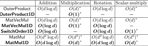
In this subsection, we compare the complexities of the techniques described in Section 3.1 and Section 3.2, in terms of homomorphic operations. For details on effect of these operations on noise and their running time, we refer the readers to [15, Table 1]. In Table 1, we have summarized the complexities for all the matrix operations. It can be easily
Table 1.Complexity of Matrix Operations in terms of Homomorphic Operations.dis the size of matrix dimensions and “−” denotes that the operation is not used. The rows corresponding to our techniques are shown in bold face.
Addition Multiplication Rotation Scalar-multiply OuterProduct O(dlogd) O(d)∗ O(dlogd) O(d)∗ OuterProduct1D − O(1)∗ − −
MatVecMul O(dlogd) O(d)∗ O(dlogd) O(d)∗ MatVecMul1D O(logd) O(1)∗ O(logd) − SwitchOrder1D O(logd) − O(logd) O(1)∗
MatMul O(d2logd) O(d2)∗ O(d2logd) O(d2)∗ MatMul1D O(dlogd) O(d)∗ O(dlogd) O(d)∗
∗: represents that the depth complexity of the operation isO(1)
observed that for all the matrix operations, our method has decreased the complexity by a factor of matrix dimension i.e.d.
4
Secure computation in the cloud
Having defined the matrix primitives in the previous section, we are now ready to proceed to defining protocols for secure computation in the cloud. We showed in the previous section that our method for matrix operations can result in significant performance improvement. Therefore, we adapt thePrivatePCAandPrivateLRprotocols proposed in [16] to work with our method for secure matrix operations. The protocols used are basically the same, except we have used our method for matrix operations. Before we proceed with their description, we first describe the input data that will be computed upon:
– We perform statistical procedures on datasets with entries in the real domain. Since the BGV scheme only works on integers, we first need to convert all the real attributes of a dataset into integers with fixed point precision. Givenx∈R, we scale it up by the magnifying constantM and then round it to the nearest integer i.e.bM xe. For the rest of description, we assume that we are computing statistics on datasets with integer attributes.
– Our setup assumes that the data rows could be coming from different sources that require that their data remains secure from other sources and the cloud. To keep the data secure, each source can encrypt their data rows separately, and send them to the cloud. But there is a problem that given the dataset (X,y) ={xT
i, yi} N−1
i=0 ∈Z
N×d t , it will
be too inefficient to compute XTXor XTy homomorphically for any practicalN. To overcome this problem, we use the fact that XTX = PN−1
i=0 xixTi and XTy =
PN−1
i=0 yixTi. Therefore, each source can encrypt the matrix xixTi and the vector yixTi for each data row independent of other sources, which can then be added in the cloud
Remark 2. Since we use the protocols proposed by Lu et al., with the exception of underlying matrix operations, we defer the security analysis of the protocols to [16, Section VI].
4.1 PrivatePCA
In this subsection, we want to compute the principal components of the data matrixX∈ZN×d
t securely in the cloud,
which requires to compute the covariance matrixΣ= N1XTX−µµT. Since we can’t perform division while computing µT and 1
NX
TXin the cloud, we rather calculate N2Σ, multiplyingXTXbyN and computingNµT in place ofµT. This works because scaling a matrix doesn’t change the direction of its eigen-vectors, it only scales their associated eigen-values. To compute N2µµT, we first compute NµT in row-wise packing, use SwitchOrder1D procedure to get
Nµ in column-wise packing, and then input both the ciphertexts into OuterProduct1D to get an encrypted matrix forN2µµT. Having computed N2Σ, all that is left is to multiply the vector v with matrixN2Σ repeatedly. Since
N2Σ is a symmetric matrix, we can do it directly with MatVecMul1Dprocedure without the need ofSwitchOrder1D
procedure. The description of the protocol is given in Algorithm 10.
Algorithm 10PrivatePCA({ct1(xTi),ct(xixTi)} N−1
i=0 , T) Input:
– ct1(xTi) : row-wise encryption ofi-th row ofX
– ct(xixTi) : ciphertext of outer-product ofxTi with itself
– T : number of iterations Output:
– u1, λ1: first principal component ofXand its magnitude Cloud:
1: ct1(NµT) =PN−1
i=0 ct1(x
T
i) . NµT∈Zdt
2: ct2(Nµ) =SwitchOrder1D(ct1(NµT))
3: ct(N2µµT) =OuterProduct1D(ct2(Nµ),ct1(NµT))
4: ct(N2Σ) =N·PN−1
i=0 ct(xix
T
i)−ct(N2µµT) . N2Σ∈Zdt×d
5: fori= 1 toT do 6: if iisoddthen
7: ct2(v(i)) =MatVecMul1D(ct(N2Σ),ct1(v(i−1))) 8: else if iiseventhen
9: ct1(v(i)) =MatVecMul1D(ct(N2Σ),ct2(v(i−1))) 10: end if
11: end for
12: if T isoddthen
13: returnct2(v(T)) andct1(v(T−1)) 14: else if T iseventhen
15: returnct1(v(T)) andct2(v(T−1)) 16: end if
Decryptor:
1: returnu1=v(T)/kv(T)kandλ1=kv(T)k/(N2· kv(T−1)k)
In this way, we can securely compute thefirstprincipal component of data matrixX. Apart from thePowerMethod
that we have in place in the form of PrivatePCA, we just need the EigenShift procedure to compute other principal components securely. TheEigenShiftprocedure is easily performed in the cloud through simple operations like matrix addition and homomorphic multiplication, along with outer product onui’s which can be done exactly like we did on Nµ.
Remark 3. If the input data is known to be normalized beforehand, we can skip the computation ofN2µTµsince it will always be zero. Moreover, we don’t need to multiplyXTXwithN then.
4.2 PrivateLR
To perform Linear Regression on the dataset (X,y) ={xT
i, yi} N−1
i=0 ∈Z
N×d
t , we need to computew= (XTX)−1XTy.
Since we can construct encrypted matricesXTXandXTyin the cloud by adding the inputsx
ixTi andyixTi respectively,
3 for matrix inversion, that involves just matrix multiplications and additions. Hence, we can use our proposed matrix operations to compute Linear Regression securely. We also need the dominant eigen valueλof matrix XTX∈ Z(td−1)×(d−1)for stable geometric convergence, which we can get through the PCA protocol before performing Linear
Regression. For the scalarλ∈Zt, we use the notation ct(λ) to refer to the ciphertext of a plaintextVwithλpacked
in each plaintext slot i.e.V[i, j] =λ. ThePrivateLRprotocol is described in Algorithm 11.
Algorithm 11PrivateLR({ct1(yixiT),ct(xixTi)} N−1
i=0 ,ct(λ), T) Input:
– ct1(yixTi) : row-wise encryption ofi-th row ofXmultiplied withi-th element ofy
– ct(xixTi) : ciphertext of outer-product ofxTi with itself
– ct(λ) : ciphertext of dominant eigen-value ofXTX – T : number of iterations
Output:
– w: weight vectorw∈Zdt−1
Cloud:
1: ct1(XTy) =PN−1
i=0 ct1(yix
T
i) .XTy∈Z(td−1)
2: ct(A0) =ct(XTX) =PN−1
i=0 ct(xixTi) .X
T
X∈Z(td−1)×(d−1)
3: ct(R0) =ct(I), ct(α(0)) =ct(λ) 4: fori= 1 toT do
5: ct(B) = 2·ct(α(i−1))·I−ct(A(i−1)) 6: ct(R(i)) =MatMul1D(ct(R(i−1)),ct(B)) 7: ct(A(i)) =MatMul1D(ct(A(i−1)),ct(B)) 8: ct(α(i)) =ct(α(i−1))·ct(α(i−1))
9: end for .ct(λ2T(XTX)−1) =ct(R(T))
10: ct2(λ2Tw) =MatVecMul1D(ct(λ2T(XTX)−1),ct1(XTy))
11: returnct2(λ2Tw) andct(λ2T) .ct(α(T)) =ct(λ2T)
Decryptor:
1: returnwfromλ2Twby dividing with λ2T.
Remark 4. We have described the protocols as if each data row is coming from an independent source. In practice, we will have multiple data rows coming from a particular source. The sources can send just one ciphertext each for
xT
i,xixTi andyixTi by performing addition corresponding to their data rows in the plaintext.
5
Choosing the right context
The right choice of context parameters can significantly improve the performance of our protocols. Choosing the right parameters is a non-trivial task inHEliband in most works usingHElib, the authors do not describe how they chose the optimal parameters for their application. In this section, we describe the theory used to choose optimal parameters for our setup. Moreover, we found that the parameter choice in [16] is non-optimal. So, we describe how to choose the right parameters for their setup as well.
As described in Section 2.1,{f1, . . . , fn}is the generating set ofZ∗m/hti. Let the order offiinZ∗m/ht, f1, . . . , fi−1ibe
mi. Therefore, we have the number of plaintext slots`=|Z∗m/hti|=
Qn
i=1mi. For efficient data movement operations,
we basically have two main requirements:
1. For eachi∈[n], we should haveordZ∗
m(fi) =mi, since it allows true rotations on slots. 2. `should be kept close to the number of plaintext slots required by the application.
For more details on why we have these requirements, refer [14, Section 4]. Before proceeding to the solution that satisfies the above-mentioned requirements, we derive some results on which our solution will be based.
Theorem 1. LetGbe a finite abelian group. Suppose we have an elementg∈Gand a subgroupN such thatord(g) =k
and|N|=K. Then the following holds:
Proof. It is clear from the definition of a quotient group that:
ordG(g) =ordG/N(g)⇐⇒ hgi ∩N={e},
where e is the identity element of G. Therefore, to prove the theorem, it is sufficient to prove that gcd(k, K) = 1 implies hgi ∩N = {e}. Let g0 be an arbitrary element ∈ hgi ∩N. This implies that ord(g0)|k as well as ord(g0)|K. Since gcd(k, K) = 1, g0 has order 1, implyingg0 =e. Since we assumed g0 to be a general element inhgi ∩N, we have hgi ∩N={e}.
Corollary 1. Let g ∈ G be an element of a finite abelian group G with ord(g) = k. Suppose we have n elements
g1, . . . , gn∈Gwithord(gi) =ki. We denote the subgroup generated by the set{g1, . . . , gn}withNi.e.N =hg1, . . . , gni.
Then the following holds:
∀i∈[n],gcd(ki, k) = 1 =⇒ ordG(g) =ordG/N(g)
Proof. It is a well-known equality that given subgroupsN1, N2/ G, we have a subgroupN1N2={h1h2|h1∈N1, h2∈
N2} such that |N1N2| = |N1| · |N2|/|N1∩N2|. Therefore, we have a subgroup N generated by {gi}ni=1 of order K which divides the product of allki’s i.e.K|(Qn
i=1ki). Since∀i∈[n],gcd(ki, k) = 1, we have gcd(k, K) = 1. Hence, by Theorem 1, the proof is complete.
5.1 For Lu et al.’s Method
For our application using Lu et al.’s method, we need a one-dimensional array of sizem1, wherem1is greater than and close tod. Moreover, this dimension should be agood dimension. These two conditions satisfy our above-mentioned requirements for efficient data movement. We achieve these conditions by choosingmandt such that:
1. m=k·m1+ 1∈P, 2. gcd(k, m1) = 1, 3. ord(t) =k.
Since m is chosen to be a prime, Z∗m is a cyclic group of order m1·k. This ensures that it has an element f1 of order m1. If we choose an element of order k (exists because Z∗m is cyclic) as t, then the number of plaintext slots ` = |Z∗m/hti| = m1. Given gcd(k, m1) = 1, by Corollary 1, we get ordZm∗(f1) = ordZ∗m/hti(f1) = m1. Therefore, Z∗m/hti=hf1iand we get a one-dimensional array with agood dimension of sizem1.
5.2 For Our Method
The optimal parameters for our method lead to atwo-dimensional hypercube with good dimensions of sizem1 and
m2, wherem1=dandm2is greater than and close tod. These parameters satisfy the requirements for efficiency, and are achieved by choosingmand tsuch that:
1. m=k·m1·m2+ 1∈P,
2. gcd(k, m1) = gcd(k, m2) = gcd(m1, m2) = 1, 3. ord(t) =k.
SinceZ∗m is a cyclic group of orderk·m1·m2, we can find f1 andf2 in Z∗m with orderm1 and m2 respectively. For a chosent of orderk, we have`=|Z∗
m/hti|=m1·m2. Given gcd(k, m1) = 1 and gcd(k, m2) = gcd(m1, m2) = 1, by Corollary 1, we get ordZ∗
m(f1) = ordZ∗m/hti(f1) = m1 and ordZ∗m(f2) =ordZ∗m/ht,f1i(f2) =m2 respectively. Therefore, Z∗m/hti=hf1, f2iand we get atwo-dimensional hypercube withgood dimensions of sizem1 andm2.
5.3 CRT method for plaintext modulus
In HElib, the maximum plaintext precision is 60 bits, which is not sufficient for our applications. To address this problem, we split the plaintext modulus t into e different primes ti each of bitsize ¡ 60 bits such that t = Qe
i=1ti for some e∈Z. Now, we create e different instances of the cryptosystem, with i-th instance operating on plaintext modulusti, and encrypt our inputs in each one of them. Then, the protocol is performed for every instance and the decryption results are combined using the Chinese Remainder Theorem to get plaintext precision of Qe
i=1blog2(ti)c bits. Using the CRT method, we essentially haveeciphertexts as opposed to one. This does not pose a problem since the CRT method is completely parallelizable. Moreover, increasingeleads to a smallerti, and as a result, lesser number of levelsL. Therefore, we get a more efficient implementation, given we have enough CPU cores.
Remark 6. In practice, we want to choose eachti ofp-bits, and to maintain security,m is chosen to be greater than a lower bound which depends ont and the number of levelsL. To choose each ti, we search the equivalence class of elements with orderkfor distinct p-bit members. The numbermis chosen such thatm1 andm2 are close todwhile keepingmas close to the lower bound as possible.
6
Implementation Details and Results
We implemented the protocols defined in Section 4 using both our method and Lu et al.’s method. The implementations were written in C++ and compiled with g++ 4.8.5. We usedHElib [14] for the implementation of the BGV scheme. Our experiments ran on a machine with Intel(R) Xeon(R) [email protected] processor and 1TB memory running CentOS 7.5.1804. In all our experiments, we use CRT method withe= 8 (see Section 5.3), and have parallelized the implementations over 8 threads.
6.1 Experimental Setup
Our experimental setup is identical to the one used in [16]. We have conducted our experiments on five datasets from the UCI Machine Learning Repository [8]. For the analysis of the effect of number of iterations and different magnification constants on performance, experiments were performed on theadult dataset that hasN = 32561 records withd= 6 numerical attributes each. More specifically, we took iteration numbersT ={3,4,5}forPrivatePCAprotocol and iteration numbersT ={1,2,3}for PrivateLRprotocol. Three magnification constants M ={10,100,1000} were considered for both the protocols. Experiments on the other datasets serve to show the scalability of our approach and we have takenT = 5, M = 1000 and T = 3, M = 1000 for PrivatePCA and PrivateLR protocol, respectively on these datasets. Following the experimental setup of [16], we have also performed all our experiments on normalized datasets, with the assumption that the data is coming from a single source. Since our experimental setup is identical to Lu et al.’s, we defer to [16, Appendix A] for discussion on iteration-error tradeoffs.
6.2 Selection of Parameters
Our parameter selection basically involves choosingmandtithat define the plaintext spacesZ[X]/(Φm(X), ti) for 1≤
i≤e, andLwhich defines the number of levels. Given a dataset with each entry bounded byB, we get a lower bound on the bitsizepofti from the inequalityti>(B2M N d)T /8for thePrivatePCA protocol andti> M1/8(B2M N d)2
T/8
for thePrivateLR protocol. An ephemeralp-bit prime following this inequality is sampled and a dry run is performed to find the required number of levelsL.
According to the analysis of [11, Appendix C.3], we get κ-bit security from the BGV scheme if the following inequality holds:
φ(m)> (L(logφ(m) + 23)−8.5)(κ+ 110)
7.2 .
Remark 7. We have chosen the best possible plaintext dimensions for our experiments. We could easily find such parameters since the matrix dimension was not too large (≤20). For operations on matrices with large dimensions, we can relax the upper bound on the size of plaintext dimensions, or we can use the block matrix multiplication method.
For other parameters inHElib, we use the default values such asσ= 3.2 (standard deviation parameter for error distribution), H = 64 (Hamming weight of secret key), r= 1 (lifting factor) and c = 3 (number of columns in key switching matrix). For all the experiments, we have maintained a minimum security of 128 bits.
6.3 Results and Analysis
In Table 2 and Table 3, we have compared the performance of our method with Lu et al.’s method for performing
PrivatePCAand PrivateLRrespectively. For PrivatePCA, we have only considered the time taken to compute the first principal component, and for PrivateLR, we exclude the time taken to compute the first eigen value λ1. From the results of Table 2 and Table 3, the following observations can be made:
– Encryption Time: The encryption time for our method isdtimes faster than Lu et al.’s on an average because we requireone ciphertext to encrypt a matrix, as opposed todciphertexts for their method.
– Evaluation Time: The difference in homomorphic evaluation time is in accordance with the complexities of matrix operations described in Table 1. As expected, the evaluation time of our method isdtimes faster than Lu et al.’s.
– Decryption Time: Since the output of both the protocols is a vector, our method outputs the same number of ciphertexts as Lu et al.’s method. Our decryption time is more, owing to the fact that the decoding operation takes more time for our method, given we are using more plaintext slots.
– Depth Requirement: Our method has comparatively less depth requirement. This is due to the fact that the
MatVecMulprocedure requires an additional scalar-multiplication operation, which adds moderate noise (see [15, Table 1]), compared to theMatVecMul1Dprocedure. This effect is more pronounced inPrivatePCAsince it involves the matrix vector multiplication in each iteration, whilePrivateLRinvolves it only once.
7
Conclusion and Future Work
We made the protocols for PCA and Linear Regression, proposed in [16], more efficient by improving their underlying matrix operations by a factor of data dimension. This was achieved by utilising the hypercube structure of the plaintext slots. Our techniques for matrix operations are flexible and can be used for any application involving matrix operations. In addition to this, we show how to choose optimal parameters for our method as well as for the method proposed in [16] by Lu et al. With our improved matrix procedures, we reduced the evaluation time of largest case (d= 20, N = 1994, M = 1000, T ={5}) for PCA from 149 seconds to 6.5 seconds, and of largest case (d= 20, N = 1994, M = 1000, T ={3}) for Linear Regression from 4400 seconds to 207 seconds. With this work, we show that the plaintext space can be utilized to a larger extent, leading to much faster PCA and Linear Regression computation.
A direction for future work is the extension of the hypercube structure fromtwo tothree-dimensions. As a result, we can reduce the complexity of matrix multiplication fromO(dlogd) to O(logd), wheredis the matrix dimension. This can be done by constructing a multiplication procedure along the lines of DNS algorithm [7]. A limitation of this approach is that it will be harder for us to find optimal parameters. A future work can explore the situations where it is beneficial to use a higher dimension plaintext structure. In this paper, we’ve considered predictive statistics through exact arithmetic and controlled the high plaintext modulus growth by using the CRT method and leveraging multiple cores to limit the impact. Switching to a scheme that allowsapproximate arithmetic, like the one described in [6], can help resolve this problem. Encoding techniques that better utilise the finite field structure of a plaintext slot can also help in containing the large plaintext modulus.
8
Acknowledgement
Table 2.Performance comparison for thePrivatePCAprotocol of our method (Section 4.1) with Lu et al.’s method ([16, Section V.C], with our optimized parameters) to find the first principal component. For all the experiments, we split the plaintext modulus into 8 primest1, . . . , t8 using our CRT method and use 8 threads to execute them all in parallel. The performance for our method is shown in bold face.
Dataset details Exp. Settings BGV settings Performance (seconds)
Dataset N d M T blog2(ti)c m L Encryption Hom. Eval. Decryption Total time
adult 32561 6 10
3 11 12703 11 0.4788 5.4683 0.1319 6.079
11047 9 0.0912 0.8562 0.2713 1.2187
4 12 14503 13 0.5767 8.8194 0.1363 9.5324
13063 11 0.1161 1.529 0.2893 1.9344
5 15 18583 17 1.2227 22.8318 0.2323 24.2868 15331 13 0.1469 2.2915 0.5591 2.9975
100
3 11 12703 11 0.4788 5.4683 0.1319 6.079
11047 9 0.0912 0.8562 0.2713 1.2187
4 14 14683 13 0.5288 9.0437 0.1364 9.7089
14071 11 0.1199 1.7285 0.296 2.1444
5 17 23011 21 1.4851 30.8704 0.2728 32.6283 15331 13 0.1423 2.3695 0.5595 3.0713
1000
3 11 12703 11 0.4788 5.4683 0.1319 6.079
11047 9 0.0912 0.8562 0.2713 1.2187
4 15 14683 13 0.6396 8.9445 0.2 9.7841
14071 11 0.1328 1.7843 1.1814 3.0985
5 19 25603 23 1.6289 33.835 0.4118 35.8757
19447 17 0.2769 5.5374 0.6144 6.4287
auto-mpg 398 7 1000 5 15 19069 17 1.3713 33.1703 0.2885 34.8301 15401 13 0.1583 2.5215 1.3696 4.0494
winequality 4898 12 1000 5 18 26293 23 3.4114 84.1018 0.5672 88.0804 19501 15 0.2865 5.3242 2.2644 7.8751
forestfires 517 13 1000 5 16 20749 19 3.074 82.9019 0.4014 86.3773 15107 13 0.1651 2.9428 1.4105 4.5184
communities 1994 20 1000 5 17 22741 21 5.1348 148.784 0.6661 154.5849 18061 15 0.2803 6.3988 2.09 8.7691
References
1. Boneh, D., Goh, E.J., Nissim, K.: Evaluating 2-dnf formulas on ciphertexts. In: Proceedings of the Second Inter-national Conference on Theory of Cryptography. pp. 325–341. TCC’05, Springer-Verlag, Berlin, Heidelberg (2005). https://doi.org/10.1007/978-3-540-30576-7 18,http://dx.doi.org/10.1007/978-3-540-30576-7_18
2. Bost, R., Popa, R.A., Tu, S., Goldwasser, S.: Machine learning classification over encrypted data. In: 22nd Annual Network and Distributed System Security Symposium, NDSS 2015, San Diego, California, USA, February 8-11, 2015 (2015),https: //www.ndss-symposium.org/ndss2015/machine-learning-classification-over-encrypted-data
3. Brakerski, Z., Gentry, C., Vaikuntanathan, V.: (leveled) fully homomorphic encryption without bootstrapping. In: Proceed-ings of the 3rd Innovations in Theoretical Computer Science Conference. pp. 309–325. ITCS ’12, ACM, New York, NY, USA (2012). https://doi.org/10.1145/2090236.2090262,http://doi.acm.org/10.1145/2090236.2090262
4. Brakerski, Z., Vaikuntanathan, V.: Fully homomorphic encryption from ring-lwe and security for key dependent messages. In: Rogaway, P. (ed.) Advances in Cryptology – CRYPTO 2011. pp. 505–524. Springer Berlin Heidelberg, Berlin, Heidelberg (2011)
5. Cheon, J.H., Kim, M., Kim, M.: Optimized search-and-compute circuits and their application to query evalua-tion on encrypted data. IEEE Transacevalua-tions on Informaevalua-tion Forensics and Security 11(1), 188–199 (Jan 2016). https://doi.org/10.1109/TIFS.2015.2483486
Table 3.Performance comparison for thePrivateLRprotocol of our method (Section 4.2) with Lu et al.’s method ([16, Section V.C], with our optimized parameters). We excluded the computational time required to compute the largest eigen-valueλ1. For all the experiments, we split the plaintext modulus into 8 primest1, . . . , t8using our CRT method and use 8 threads to execute them all in parallel. The performance for our method is shown in bold face.
Dataset details Exp. settings BGV settings Performance (Seconds)
Dataset N d M T blog2(ti)c m L Encryption Hom. Eval. Decryption Total time
adult 32561 6 10
1 11 10531 9 0.4964 3.8267 0.0733 4.3964
8311 7 0.1959 0.6444 0.1471 0.9874
2 15 13121 11 0.5524 28.1256 0.1198 28.7978 10771 9 0.2719 4.7969 0.2767 5.3455
3 26 23741 21 1.8307 159.8920 0.2256 161.9483 20731 19 0.7658 34.0543 0.6125 35.4326
100
1 11 10531 9 0.4964 3.8267 0.0733 4.3964
8311 7 0.1959 0.6444 0.1471 0.9874
2 17 15031 13 0.6564 33.8865 0.1153 34.6582 14011 11 0.2912 6.5338 0.3211 7.1461
3 30 27011 23 1.8077 188.1300 0.2712 190.2089 23011 21 0.7817 38.3839 0.6418 39.8074
1000
1 11 10531 9 0.4964 3.8267 0.0733 4.3964
8311 7 0.1959 0.6444 0.1471 0.9874
2 19 17011 15 1.2712 60.1418 0.1906 61.6036 14731 13 0.3093 7.4470 0.3506 8.1069
3 33 28111 25 2.0766 206.4470 0.2745 208.7981 26431 23 0.9210 45.4241 0.6954 47.0405
auto-mpg 398 7 1000 3 26 24007 21 2.0630 228.9190 0.2190 231.2010 21211 19 0.8031 49.1406 0.6096 50.5533
winequality 4898 12 1000 3 30 26203 23 3.5929 1169.4800 0.3569 1173.4298 23629 21 0.8884 95.7648 3.1740 99.8228
forestfires 517 13 1000 3 27 25117 23 3.8555 1158.9700 0.3843 1163.2098 22621 21 0.8640 122.2040 2.9421 126.0101
communities 1994 20 1000 3 29 27361 23 6.0348 4399.6500 0.4428 4406.1276 26981 21 0.9311 207.5400 4.2580 212.7291
7. Dekel, E., Nassimi, D., Sahni, S.: Parallel matrix and graph algorithms. SIAM Journal on Computing10(4), 657–675 (1981). https://doi.org/10.1137/0210049,https://doi.org/10.1137/0210049
8. Dheeru, D., Karra Taniskidou, E.: UCI machine learning repository (2017),http://archive.ics.uci.edu/ml
9. Fox, G., Otto, S., Hey, A.: Matrix algorithms on a hypercube i: Matrix multiplication. Parallel Computing 4(1), 17 – 31 (1987). https://doi.org/https://doi.org/10.1016/0167-8191(87)90060-3,http://www.sciencedirect.com/science/ article/pii/0167819187900603
10. Gentry, C.: Fully homomorphic encryption using ideal lattices. In: Proceedings of the Forty-first Annual ACM Symposium on Theory of Computing. pp. 169–178. STOC ’09, ACM, New York, NY, USA (2009). https://doi.org/10.1145/1536414.1536440,http://doi.acm.org/10.1145/1536414.1536440
11. Gentry, C., Halevi, S., Smart, N.P.: Homomorphic evaluation of the aes circuit. In: Safavi-Naini, R., Canetti, R. (eds.) Advances in Cryptology – CRYPTO 2012. pp. 850–867. Springer Berlin Heidelberg, Berlin, Heidelberg (2012)
12. Graepel, T., Lauter, K., Naehrig, M.: Ml confidential: Machine learning on encrypted data. In: Proceedings of the 15th International Conference on Information Security and Cryptology. pp. 1–21. ICISC’12, Springer-Verlag, Berlin, Heidelberg (2013). https://doi.org/10.1007/978-3-642-37682-5 1,http://dx.doi.org/10.1007/978-3-642-37682-5_1
13. Guo, C., Higham, N.: A schur-newton method for the matrix pth root and its inverse. SIAM Journal on Matrix Analysis and Applications28(3), 788–804 (2006). https://doi.org/10.1137/050643374,https://doi.org/10.1137/050643374 14. Halevi, S., Shoup, V.: Design and implementation of a homomorphic-encryption library (2013),http://people.csail.mit.
edu/shaih/pubs/he-library.pdf
16. Lu, W., Kawasaki, S., Sakuma, J.: Using fully homomorphic encryption for statistical analysis of categorical, ordinal and numerical data (this is the full version of the conference paper presented at NDSS 2017). IACR Cryptology ePrint Archive, Report 2016/1163 (2016),https://eprint.iacr.org/2016/1163
17. Naehrig, M., Lauter, K., Vaikuntanathan, V.: Can homomorphic encryption be practical? In: Proceedings of the 3rd ACM Workshop on Cloud Computing Security Workshop. pp. 113–124. CCSW ’11, ACM, New York, NY, USA (2011). https://doi.org/10.1145/2046660.2046682,http://doi.acm.org/10.1145/2046660.2046682
18. Paillier, P.: Public-key cryptosystems based on composite degree residuosity classes. In: Stern, J. (ed.) Advances in Cryp-tology — EUROCRYPT ’99. pp. 223–238. Springer Berlin Heidelberg, Berlin, Heidelberg (1999)
19. Rivest, R.L., Shamir, A., Adleman, L.: A method for obtaining digital signatures and public-key cryptosystems. Commun. ACM21(2), 120–126 (Feb 1978). https://doi.org/10.1145/359340.359342,http://doi.acm.org/10.1145/359340.359342 20. Smart, N.P., Vercauteren, F.: Fully homomorphic encryption with relatively small key and ciphertext sizes. In:
Proceed-ings of the 13th International Conference on Practice and Theory in Public Key Cryptography. pp. 420–443. PKC’10, Springer-Verlag, Berlin, Heidelberg (2010). https://doi.org/10.1007/978-3-642-13013-7 25, http://dx.doi.org/10.1007/ 978-3-642-13013-7_25
21. Smart, N.P., Vercauteren, F.: Fully homomorphic simd operations. Des. Codes Cryptography 71(1), 57–81 (Apr 2014). https://doi.org/10.1007/s10623-012-9720-4,http://dx.doi.org/10.1007/s10623-012-9720-4
22. Wu, D., Haven, J.: Using homomorphic encryption for large scale statistical analysis (2012),https://crypto.stanford. edu/~dwu4/FHE-SI_Report.pdf
23. Yasuda, M., Shimoyama, T., Kogure, J., Yokoyama, K., Koshiba, T.: Secure pattern matching using somewhat homomorphic encryption. In: Proceedings of the 2013 ACM Workshop on Cloud Computing Security Workshop. pp. 65–76. CCSW ’13, ACM, New York, NY, USA (2013). https://doi.org/10.1145/2517488.2517497, http://doi.acm.org/10.1145/2517488. 2517497
![Table 2. Performance comparison for theV.C], with our optimized parameters) to find the first principal component](https://thumb-us.123doks.com/thumbv2/123dok_us/7975912.1322600/16.595.68.531.116.501/table-performance-comparison-optimized-parameters-rst-principal-component.webp)
![Table 3. Performance comparison for the PrivateLR protocol of our method (Section 4.2) with Lu et al.’s method ([16, SectionV.C], with our optimized parameters)](https://thumb-us.123doks.com/thumbv2/123dok_us/7975912.1322600/17.595.68.529.117.503/performance-comparison-privatelr-protocol-section-sectionv-optimized-parameters.webp)
