Validation of Selected Non-destructive Methods for Determining the Compressive Strength of Masonry Units Made of Autoclaved Aerated Concrete

Article

Validation of Selected Non-destructive Methods for

Determining the Compressive Strength of Masonry

Units Made of Autoclaved Aerated Concrete

Radosław Jasiński1*_{, Łukasz Drobiec} 2 _{and Wojciech Mazur} 3

1 _{Silesian University of Technology, Department of Building Structures; ul. Akademicka 5, 44-100 Gliwice,}

Poland [email protected] (R.J.)

2 _{Silesian University of Technology, Department of Building Structures; ul. Akademicka 5, 44-100 Gliwice,}

Poland [email protected] (Ł.D.)

3 _{Silesian University of Technology, Department of Building Structures; ul. Akademicka 5, 44-100 Gliwice,}

Poland [email protected] (W.M.)

* Correspondence: [email protected]; ORCID: https://orcid.org/0000-0003-4015-4971; Tel. +48 32 237-11-27

Abstract: Semi-destructive and non-destructive techniques are not commonly used for masonry as they are complex and difficult to perform. This paper describes validation of the following methods: semi-destructive and non-destructive, ultrasonic technique for autoclaved aerated concrete (AAC). The research subject was the compressive strength of AAC test elements with declared various density classes of: 400, 500, 600 and 700 (kg/m3_{) and various moisture levels.}

Empirical data including the shape and size of specimens, were established from tests on 494 cylindrical and cuboid specimens, and standard cube specimens 100×100×100 mm using the general relationship for standard concrete (Neville’s curve). The effect of moisture on AAC was taken into account while determining the strength fBw for 127 standard specimens tested at

different levels of water content (w = 100%, 67%, 33% 23% and 10%). Defined empirical relations can be used to correct the compressive strength of dry specimens. For 91 specimens 100×100×100 mm, the P-wave velocity cp was tested with the transmission method using using the ultrasonic

pulse velocity method with exponential transducers. The curve (fBw – cp) for determining the

compressive strength of AAC elements with any moisture level (fBw) was established.

Keywords: Autoclaved Aerated Concrete (AAC), Compressive Strength, Shape and Size of Specimen, Moisture of AAC, Ultrasonic Testing

1. Introduction

Non-destructive (ultrasonic, sclerometric, pull-out and pull-off) methods for determining mechanical parameters are not commonly used for masonry structures due to significant variations of materials, technology and performance [1-4]. In-situ evaluation of masonry compressive strength can be performed using the destructive (direct) method with flat jacks or drilling a fragment of the masonry [5]. The semi-destructive method consists in testing small specimens of masonry or its components (elements of masonry and mortar) and applying proper empirical curves to convert obtained strength values into the requested value fk [6]. Also, stricte non-destructive methods, such

as sclerometic ones (L-type Schmidt hammer) and ultrasonic methods are undertaken although they are not common now.

Determination of compressive strength of modern masonry walls with thin joints, where mortar levels any irregularities of support areas and head joints are unfilled, requires only the properly determined compressive strength of the masonry unit fB and calculated (with empirical

factors ηw and δ expressing the specimen moisture and shape) an average normalised compressive

strength. This procedure involves the relationship acc. to Eurocode 6 [7] and is used to calculate the specific compressive strength of the masonry wall:

(

)

( )

0 B w 85

0, , ,

b

k Kf K f K f

f = =





where: K = 0.75 or 0.8, fb– average normalised compressive strength of masonry unit determined for

specimens 100×100×100 mm, fB – average compressive strength of the whole masonry unit or a

specimen with moisture content w = 0, fBw– compressive strength of the masonry specimen cut out

from the masonry construction with the actual moisture content.

If tests are performed on specimens having different dimensions than a cube with a 10 mm side, the normalised strength is determined using δ factors specified in the standard PN-EN 772-1 [8]. However, the standard does not specify conversion factors for non-standard specimens, such as cores or micro-cores. Consequently, the conversion of results is burdened with a default error that is difficult to be estimated. The literature [9-11] describes conversion factors obtained from tests on other materials, such as concrete, ceramics, or masonry units [12]. No relations to AAC have been presented so far. There are no procedures for determining specific compressive strength of the existing masonry wall with the actual density and moisture content. But in some situations, drilling micro-cores, and even performing sclerometic tests is impossible. So, only ultrasonic non-destructive technique can be used to determine compressive strength.

This paper describes an attempt to establish the empirical curve for determining the normalised compressive strength of the AAC masonry unit with unspecified density and moisture content fBw using semi-destructive techniques. Neville’s curve [9] , in the commonly known form

from diagnosing standard concrete, was used and calibrated to nominal density classes of AAC (400, 500, 600 and 700). Knowing that, apart from the effect of rising and hardening [13-14], also moisture content in AAC influences the compressive strength, tests were performed and additional empirical relations were defined. The analysis included test results [15] from 494+127 cylindrical and cuboid specimens used to develop empirical curves. Results obtained from destructive tests on standard cube specimens 100×100×100 mm at different moisture content were correlated with results from testing velocity of P-wave generated by point transducers with the transmission method.

2. Semi-destructive technique

2.1. Specimens, a technique and test results for specimens with varying shapes and dimensions

Tests included four series of masonry units with thickness within the range of 180 mm-240 mm and different classes of density: 400, 500, 600 and 700, from each 20 masonry units were randomly selected. Six series of cores with varying diameters were drilled from each masonry unit. Six series of square specimens having different side length and height were sampled from masonry units using a diamond saw. Cuboid specimens included blocks with dimensions of 100×100×100 mm, which were used as basic specimens for determining the strength fB in accordance with Appendix B

to the standard EN 771-4 [16]). Drilled core and cube specimens are illustrated in Fig. 1. All specimens drilled from blocks were dried until constant weight at a temperature of 105°C±5°C (for at least 36 hours).

Depending on the specimen size, loading rate was 2400 N/s and 100 N/s. Due to the size of specimens, two types of machines having an operating range of 100 kN and 3000 kN, and the class of accuracy of 0.5, were used (acc. to EN 772-1 [8]) – Fig. 2. Compressive strength fB was determined

(

a

)

(

b

)

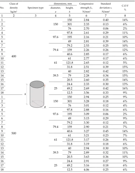
Table 1. Test results for core (cylindrical) specimens

No.

Class of density kg/m3

Specimen type

dimensions, mm Compressive strength fci,

N/mm2

Standard deviation s,

N/mm2

C.O.V % diameter,

ø

height, h

1 2 3 4 5 6 7 8

1

400

150

150 2.84 0.40 14%

2 301 2.33 0.13 6%

3 76 2.70 0.06 2%

4

97.6

97.8 2.61 0.29 11%

5 195 2.16 0.21 10%

6 49 2.81 0.39 14%

7

79.4

79.2 2.53 0.25 10%

8 159 2.26 0.26 12%

9 40.6 2.85 0.17 6%

10

61

61 2.77 0.17 6%

11 121.8 2.65 0.12 5%

12 31.8 2.51 0.39 15%

13

39.5

40 2.82 0.42 15%

14 79 2.28 0.34 15%

15 20.5 2.60 0.35 14%

16

25

24.4 2.33 0.30 13%

17 49.2 2.69 0.42 16%

18 12.5 3.56 0.33 9%

1

500

150

150 2.94 0.25 9%

2 301 3.28 0.18 6%

3 76 3.01 0.12 4%

4

97.6

97.8 2.88 0.16 6%

5 195 3.09 0.06 2%

6 49 3.15 0.29 9%

7

79.4

79.2 3.30 0.12 4%

8 159 2.90 0.21 7%

9 40.6 3.27 0.45 14%

10

61

61 3.21 0.23 7%

11 121.8 3.17 0.26 8%

12 31.8 3.19 0.18 6%

13

39.5

40 2.94 0.30 10%

14 79 2.89 0.32 11%

15 20.5 3.63 0.36 10%

16

25

24.4 2.91 0.27 9%

17 49.2 3.16 0.18 6%

cont. Table 1 Test results for core (cylindrical) specimens

1 2 3 4 5 6 7 8

1

600

150

150 5.06 0.36 7%

2 301 4.23 0.21 5%

3 76 5.11 0.68 13%

4

97.6

97.8 4.49 0.22 5%

5 195 4.26 0.18 4%

6 49 5.01 0.61 12%

7

79.4

79.2 4.43 0.09 2%

8 159 4.73 0.25 5%

9 40.6 5.14 0.52 10%

10

61

61 4.65 0.47 10%

11 121.8 4.54 0.16 3%

12 31.8 5.19 0.66 13%

13

39.5

40 4.87 0.53 11%

14 79 4.18 0.31 8%

15 20.5 6.00 0.81 14%

16

25

24.4 5.17 0.27 5%

17 49.2 4.79 0.64 13%

18 12.5 6.88 0.76 11%

1

700

150

150 7.12 0.96 14%

2 301 7.25 0.56 8%

3 76 7.69 0.63 8%

4

97.6

97.8 7.37 0.76 10%

5 195 7.22 0.42 6%

6 49 7.93 0.28 4%

7

79.4

79.2 6.77 0.35 5%

8 159 7.25 0.57 8%

9 40.6 8.87 0.36 4%

10

61

61 7.25 1.04 14%

11 121.8 7.05 0.51 7%

12 31.8 8.57 0.35 4%

13

39.5

40 7.55 0.32 4%

14 79 7.21 1.08 15%

15 20.5 9.18 0.77 8%

16

25

24.4 7.66 0.77 10%

17 49.2 7.73 0.40 5%

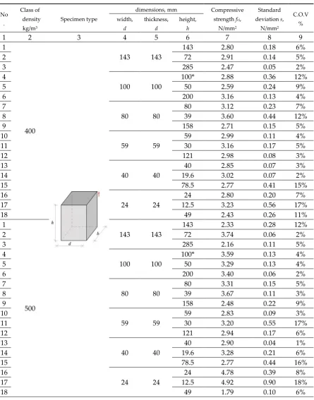
Table 2. Test results for cuboid specimens

No .

Class of density kg/m3

Specimen type

dimensions, mm Compressive strength fci,

N/mm2

Standard deviation s,

N/mm2

C.O.V % width,

d

thickness, d

height, h

1 2 3 4 5 6 7 8 9

1

400

143 143

143 2.80 0.18 6%

2 72 2.91 0.14 5%

3 285 2.47 0.05 2%

4

100 100

100* 2.88 0.36 12%

5 50 2.59 0.24 9%

6 200 3.16 0.13 4%

7

80 80

80 3.12 0.23 7%

8 39 3.60 0.44 12%

9 158 2.71 0.15 5%

10

59 59

59 2.99 0.11 4%

11 30 3.16 0.17 5%

12 121 2.98 0.08 3%

13

40 40

40 2.85 0.07 3%

14 19.6 3.02 0.07 2%

15 78.5 2.77 0.41 15%

16

24 24

24 2.80 0.20 7%

17 12.5 3.23 0.56 17%

18 49 2.43 0.26 11%

1

500

143 143

143 2.33 0.28 12%

2 72 3.74 0.06 2%

3 285 2.16 0.11 5%

4

100 100

100* 3.59 0.13 4%

5 50 3.29 0.13 4%

6 200 3.40 0.06 2%

7

80 80

80 3.31 0.15 5%

8 39 3.67 0.11 3%

9 158 2.48 0.22 9%

10

59 59

59 2.83 0.09 3%

11 30 3.20 0.55 17%

12 121 2.94 0.17 6%

13

40 40

40 2.90 0.04 1%

14 19.6 3.28 0.21 6%

15 78.5 2.77 0.44 16%

16

24 24

24 4.78 0.39 8%

17 12.5 4.92 0.90 18%

cont. Table 2 Test results for cuboid specimens

1 2 3 4 5 6 7 8 9

1

600

143 143

143 3.97 0.10 2%

2 72 5.69 0.10 2%

3 285 3.58 0.25 7%

4

100 100

100* 4.95 0.35 7%

5 50 5.80 0.35 6%

6 200 5.34 0.61 11%

7

80 80

80 6.01 0.75 12%

8 39 6.60 0.12 2%

9 158 4.45 0.19 4%

10

59 59

59 4.58 0.08 2%

11 30 5.85 0.04 1%

12 121 4.84 0.09 2%

13

40 40

40 5.81 0.41 7%

14 19.6 5.06 0.17 3%

15 78.5 5.65 0.20 4%

16

24 24

24 6.02 0.74 12%

17 12.5 6.30 0.19 3%

18 49 4.19 0.91 22%

1

700

143 143

143 4.88 1.03 21%

2 72 7.21 0.27 4%

3 285 5.28 0.44 8%

4

100 100

100* 8.11 0.58 7%

5 50 7.02 1.07 15%

6 200 7.56 0.25 3%

7

80 80

80 6.31 0.27 4%

8 39 8.79 0.89 10%

9 158 6.50 0.98 15%

10

59 59

59 5.76 0.34 6%

11 30 6.31 1.10 17%

12 121 4.65 0.95 20%

13

40 40

40 5.48 0.52 10%

14 19.6 7.00 0.22 3%

15 78.5 6.71 0.29 4%

16

24 24

24 5.38 1.98 37%

17 12.5 9.37 1.96 21%

18 49 4.89 1.66 34%

* – cube specimens according to PN-EN 771-4:2012 used to determine compressive strength fB.

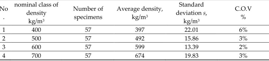
Table 3. Test results for AAC density

No .

nominal class of density

kg/m3

Number of specimens

Average density, kg/m3

Standard deviation s,

kg/m3

C.O.V %

1 400 57 397 22.01 6%

2 500 57 492 15.86 3%

3 600 57 599 13.39 2%

Development of cracks in cuboid specimens of different dimensions was recorded with an optical measuring system – Fig. 3. In dense specimens with slenderness ratio h/b = 1, diagonal cracks developed at upper edges, and they formed two truncated pyramids at failure – Fig. 3a. In specimens with slenderness ratio h/d = 2, a vertical crack in the mid-length of the base appeared as the first, and then secondary diagonal cracks formed near corners of specimens - Fig. 3b. The arrangement of cracks in specimens of bigger volume at failure was similar to dense specimens – Fig. 3c.

(

a

)

(

b

)

Figure 2. Testing compressive strength of AAC specimens [15]: (a) tests on cores using a strength testing machine with an operating range of 100 kN, (b) tests on cuboid specimens using a strength testing machine with an operating range of 3000 kN

(

a

)

(

b

)

(

c

)

Figure 3. Destruction of specimens with varying slenderness ratio [15]: (a) specimen 143×143×143 mm, (b) specimen 100×100×200 mm, (c) specimen 80×80×158 mm.

If strength of the material depends on its defects, such as pores or voids, then individual specimens of different shapes can have significantly different values. These aspects are covered by Weibull’s statistical theory of material strength [17-18], which states that strength of the material is reversely proportional to volume of the tested specimen at the same probability of failure:

m / V V 1 1 2 2 1       =  

, (2)

where: σ1, σ2– failure stresses for specimens with volume V1 and V2, m – constant.

The exponential type of this relation (2) is similar to hyperbole and is used during tests on compressive and tensile strength of dense specimens. Neville [9] developed a similar hyperbolic relation with regard to its course, while testing specimens of different slenderness. This relation is used to determine compressive strength of concrete in specimens with shape and dimensions different from those of standard specimens (blocks 150×150×150 mm). The empirical curve for standard concrete is expressed as:

d h hd V , , f f cube , c c + + = 152 697 0 56 0 150 , (3)

where: V– specimen volume, h– specimen height, d– the smallest side dimension of the specimen. Replacing strength fc,cube150 obtained from standard specimens 150×150×150 mm with strength fB

for specimens 100×100×100 mm drilled from masonry units, and the ratio 152hd with volume of the standard specimen 100hd, the relationship(3) can be expressed as:

x a b y d h hd V a b f f B

c _{→ = +}

+ + = 100 , (4)

where: fB – compressive strength of normalised specimen 100×100×100 mm with moisture content

w=0, fc– compressive strength of a specimen with any shape and dimensions, and moisture content

w=0, a and b – constant coefficients for the curve , y= f_c/f_B – ratio of compressive strength,

d / h hd / V

x= 100 + – dimensionless coefficient representing the effect of specimen volume and slenderness.

Sought parameters of the curve (4) were determined by searching a local minimum sum of squares difference:

( )



( )



i i _i

n

i i i

b x a y x y y b , a S 1 2 1

2 _{, (5)}

using the following relationships:

( )

, (6)

( )

. (7)

        −    −  = = = = = = = n i i n i i n i _i n i _i n i i n i _i i x x n x x y n x y a 1 1 1 2 1 1 1 1 1 1 1 1 1

, ₍₈₎

                       −    −  −  = = = = = = = = = n i _i n i i n i i n i _i n i i n i i n i i i n

i i x

x x n x x y n x y n y n b 1 1 1 1 2 1 1 1 1 1 1 1 1 1 1 1 1 1

. (9)

For defining compliance of the curve, some uncertainty was assumed to be neglected during measurements x (the specimen geometry). Additionally, uncertainties of all y values were the same (the same significance of measurements resulting from identical measuring techniques). To estimate the coefficient of correlation, the following was calculated:

- error of estimate

(

)

 −

= = n

i i m

tN y y

n S

1

2

1

, (10)

where: = 

= n i i m y n y 1 1 ,

- sum of errors:

 _             + − = = n

i i i

rN _x b

a y n S 1 2 1

, (11)

and then coefficient of correlation:

tN rN tN S S S

R= − . ₍₁₂₎

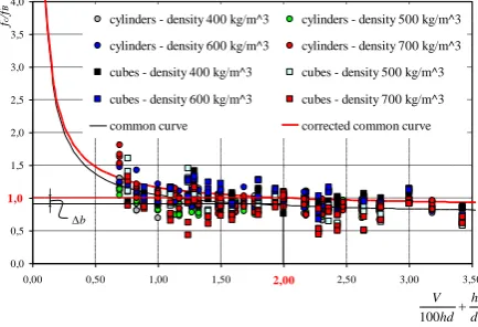
The paper [15] compares curve correlations developed for cuboid and cylindrical specimens. Obtained values of curve coefficients a and b are compared in Table 4. Comparison of test results and the common curve is shown in Fig. 4.

0,0 0,5 1,0 1,5 2,0 2,5 3,0 3,5 4,0

0,00 0,50 1,00 1,50 2,00 2,50 3,00 3,50

f

c

/f

B

cylinders - density 400 kg/m^3 cylinders - density 500 kg/m^3 cylinders - density 600 kg/m^3 cylinders - density 700 kg/m^3 cubes - density 400 kg/m^3 cubes - density 500 kg/m^3 cubes - density 600 kg/m^3 cubes - density 700 kg/m^3 common curve corrected common curve

d h hd V ₊ 100 Db 2,00 1,0

Figure 4. Test results for all core and cube specimens and determined curve of correlation

When specimens 100×100×100 mm are used, the value of curve dominator is V/100hd + h/d = 2, and strength ratios calculated according to equations from Table 4 are fc/fB≠ 1. To obtain the ratio

fc/fB = 1 from normalised specimens, curves need to be translated in parallel to the intercept axis

2 1 100 a b b d h hd V a b b f f B

c _{→ = − −}

+ +

+

= D D .

(13)

Table 4. Comparison of coefficients and equations of empirical curves Density range of

AAC, average density ρ,

(nominal class of density) kg/m3 Coefficient for curve R Additive correction factor Δb Corrected coefficient for curve bkor Curve equation

a b

from 375 to 446 397, (400)

0.159 0.857 0.324 0.06 0.921

d h hd V , , f f B c + + = 100 159 0 921 0

from 462 to 532, 492, (500)

0.312 0.682 0.533 0.16 0.844

d h hd V , , f f B c + + = 100 312 0 844 0

from 562 to 619, 599, (600)

0.349 0.779 0.612 0.05 0.826

d h hd V , , f f B c + + = 100 349 0 826 0

from 655 to 725, 674, (700)

0.454 0.608 0.614 0.16 0.773

d h hd V , , f f B c + + = 100 454 0 773 0

common curve aw = 0.321

bw =

0.730 0.262 0.11 0.840 V_{hd d}h

, , f f B c + + = 100 321 0 840 0

2.3. Calibrating a curve in air-dry conditions

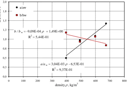
Many curves developed for specific density of AAC were replaced with a curve which was more favourable for diagnostic purposes and could be used to determine the strength of AAC with any density and moisture content. Coefficients a and b determined for concrete with specific density within the defined ranges and presented in Table 4 as well as coefficients aw and bw of the common

curve were used to develop correlations illustrated in Fig. 5.

b / bw = -9,09E-04 r + 1,49E+00

R2

= 5,44E-01

a/aw = 3,04E-03 r - 6,53E-01

R2 = 9,37E-01

0,0 0,3 0,5 0,8 1,0 1,3 1,5 1,8 2,0

0 100 200 300 400 500 600 700 800

density r, kg/m3

a /a w , b /b w a/aw b/bw Liniowy (b/bw) Liniowy (a/aw)

Figure 5. Relative coefficients of curves

The following relationships describing curve coefficients as a function of AAC densities were developed on the basis of results shown in Fig. 5, using the method of least squares:

(

)

(

)

(

)

(

)

b= w  − =−   −

−

−

_r

_r

. (15)

The formation of AAC curve with any density, when a and b values have been determined, requires a correction for the coefficient b which results in the strength ratio obtained from the curve (13) at V/100hd + h/d = 2.

2.4. Calibrating an empirical curve in moisture conditions

Properties of AAC and standard concrete depend on moisture content [14, 19] which cause a clear reduction in compressive and tensile strengths, and degradation of insulating parameters. Thus, further tests also focus on the effect of moisture content in AAC, which is a ratio of absorbed water to the mass of dry material:

%, m

m m w

s s

w − _100

= ₍₁₆₎

where: mw– mass of wet specimen, ms– mass of specimen dried until constant weight.

The maximum moisture content (absorbality) wmax in AAC corresponds to the level of water, at

which no further increase in mass mw is observed as the effect of passage of (capillary) water.

Relative moisture was calculated as the ratio of current and maximum moisture w/wmax.

The total number of 127 specimens 100×100×100 m, divided into five six-element series, was prepared from AAC blocks with varying density. Each specimen was put into containers filled with water to saturate it with water as the effect of passage of (capillary) water. Specimens were weighed every 6 hours and moisture content w was calculated each time. Maximum moisture content in each type of AAC was assumed to be determined at first, and then specimens were dried until the required moisture content. Strength tests were expected to be performed at the following levels of relative moisture: w / wmax = 100%; 67%; 33%; 23%, 10% and 0%. Average test results for individual

series of specimens are shown in Table 8.

Maximum moisture content in AAC depended on nominal density. At the density increase in the range from ρ = 397 kg/m3 _{to 674 kg/m}3_{, the maximum moisture content was varying within wmax}

= 89.9% – 53.3 %, which made it possible to determine a straight line of the least square in the following form:

34 1 1000 23

1, ,

w_{m ax}=− r + when _{3 3}

m kg 674 m

kg

397 r . (17)

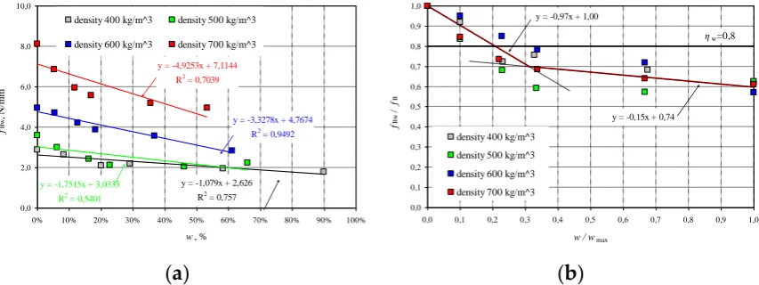
At each moisture level, destructive tests were performed to determine the strength of wet concrete fBw, and the results are illustrated in Fig. 6a as a function of moisture w. Fig. 6b presents the

obtained strength values with respect to the strength fB of dry (w=0) AAC as a function of relative

moisture w / wmax.

Two empirical lines were drawn on the basis of obtained results and used to determine the relative strength of AAC as a function of relative moisture in the following form:

   

 

+ −

= → + −

= 096 1 097 1

m ax B

Bw m ax

B Bw

w w , f f w

w , f f

when 0 0,31

w w

m ax



 ₍₁₈₎

   

 

+ −

= → + −

= 015 074 015 0,74

w w , f f , w

w , f f

m ax B

Bw m ax

B

Bw _{when 031 1,0}

w w ,

m ax



 ₍₁₉₎

Strength fBw calculated from equations (18) and (19) includes the moisture effect, so it does not

y = -1,079x + 2,626

R2 _{= 0,757}

y = -1,7515x + 3,0333 R2 _{= 0,5401}

y = -3,3278x + 4,7674 R2 _{= 0,9492} y = -4,9253x + 7,1144

R2 _{= 0,7039}

0,0 2,0 4,0 6,0 8,0 10,0

0% 10% 20% 30% 40% 50% 60% 70% 80% 90% 100%

w, %

f

Bw

,

N

/m

m

2

density 400 kg/m^3 density 500 kg/m^3 density 600 kg/m^3 density 700 kg/m^3

y = -0,97x + 1,00

y = -0,15x + 0,74

0,0 0,1 0,2 0,3 0,4 0,5 0,6 0,7 0,8 0,9 1,0

0,0 0,1 0,2 0,3 0,4 0,5 0,6 0,7 0,8 0,9 1,0

w / wmax

f

B

w

/

f

B

density 400 kg/m^3 density 500 kg/m^3 density 600 kg/m^3 density 700 kg/m^3

ηw=0,8

(

a

)

(

b

)

Figure 6. Test results for AAC strength, taking into account moisture level: (a) strength fBw as a

function of moisture w, (b) relative strength of AAC fBw / fB as a function w / wmax

Fig. 6b also shows the value of factor ηw = 0.8 recommended by the standard EN 772-1 [8] and

used to take into consideration the effect of moisture level. The standard recommendation provides the safe reduction of compressive strength only for the moisture level w / wmax = 0.2. Tests on walls

with higher moisture content showed that compressive strength could be even reduced by 40%, that is, over twice more than the provisions recommend.

Table 8. Test results for AAC with varying moisture content

No.

Density range of AAC, average density

ρ, (nominal class of

density) kg/m3

Average moisture content

w, %

Average relative moisture

w/wmax

Average compressive

strength fBw, N/mm2

Standard deviation, s, N/mm2

COV, %

Average relative compressive

strength fBw / fB

1 2 3 4 5 6 7 8

1

from 375 to 446, 397, (400),

0 0 2.88* 0.36 12% 1.0

2 8.3 0.10 2.64 0.21 8% 0.92

3 20.1 0.23 2.09 0.11 5% 0.72

4 29.1 0.33 2.18 0.16 8% 0.76

5 58.3 0.67 1.96 0.14 7% 0.68

6 89.9 1.00 1.78 0.13 7% 0.62

7

from 462 to 532, 492, (500),

0 0 3.59* 0.13 4% 1.0

8 6.2 0.10 3.00 0.22 7% 0.84

9 16.2 0.23 2.44 0.49 20% 0.68

10 22.8 0.33 2.12 0.21 10% 0.59

11 46.1 0.67 2.06 0.29 14% 0.57

12 66.0 1.00 2.24 0.23 10% 0.62

13

from 562 to 619, 599, (600),

0 0 4.95* 0.35 7% 1.0

14 5.40 0.10 4.71 0.49 10% 0.95

15 12.6 0.23 4.21 0.38 9% 0.85

16 18.2 0.34 3.88 0.52 13% 0.78

17 58.3 0.67 1.96 0.33 9% 0.68

18 61.1 1.00 2.82 0.28 10% 0.57

1 2 3 4 5 6 7 8 19

from 655 to 725, 674, (700),

0 0 8.11* 0.58 7% 1.0

20 5.30 0.10 6.86 0.63 9% 0.85

21 11.7 0.22 5.96 0.71 12% 0.74

22 16.8 0.34 5.56 0.58 10% 0.69

23 46.1 0.67 2.06 0.70 13% 0.57

24 53.3 1.00 4.95 0.41 8% 0.61

* fB– compressive strength of dry AAC, when w = 0.

To sum it up, determination of compressive strength of the wall fk requires at first, taking into

account varying shape and moisture, to estimate in-situ moisture content, and then drill specimens, estimate density and compressive strength, and then make conversion relevant to moisture. Compressive strength calculated from the equation (18) or (19) can be substituted to the equation (1).

3. Ultrasonic non-destructive method

The application of traditional cylindrical transducers may be difficult as it requires the agent coupling with the tested surface. Tests on very porous and coarse materials, such as AAC, with cylindrical transducers may be also problematic. Measuring the distance of the wave is also difficult, especially if tests are performed only at one side [21-23]. Measurements are simpler and easier to perform when transducers having local contact with concrete are applied. Waveguides for this type of transducers are in cone shape or can be formed according to the exponential curve. As energy produced by ultrasound is lower than in cylindrical transducers with a larger contact surface, the spacing of transducers at one-side access to standard concrete with density of ca. 2500 kg/m3 should not exceed 25 cm, and at both-side access - 15 cm [24].

3.1. Testing technique of specimens

Non-destructive tests on AAC were performed using the ultrasonic testing, commonly applied for testing strength of concrete [25], and testing masonry walls [1-3]. Ultrasonic testing was conducted on block specimens 100×100×100 mm drilled from masonry units – Fig. 7. Wet specimens with relative moisture w / wmax = 100%, 67%, 33%, 23% and 10%, and specimens dried until constant

weight w / wmax = 0% were used in tests. Each series of elements included at least 20 specimens, and

91 specimens in total were tested.

The PUNDIT LAB instrument (Proceq SA, Schwerzenbach, Switzerland) was utilized for measurements of the ultrasonic pulse velocity. Commercial exponential transducers with the waveguide length L = 50 mm, diameters ø1 = 4.2 mm and ø2 = 50 mm, and frequency 54 kHz were

employed. The applied research methodology and equipment was also used for testing also for ultrasonic tomography for concrete [26-27] or masonry [28-29].

Each specimen was put on a pad insulating from shock and outdoor noise, and then transducers were applied to walls and the measurement was made with the transmission method. Transducers were in contact with specimens at an angle of 90o _{within distance between transducers}

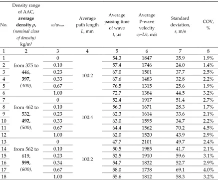
measured every time with an accuracy up to ±1 mm. Time was measured with an accuracy up to ±0,1 µs. The measurement results are presented in Table 9.

In AAC specimens dried until constant weight, the velocity of ultrasounds was varying from 1847 m/s in concrete of class 400 kg/m3 _{to 2379 m/s in concrete of class 700 kg/m}3_{. An increase in}

Figure 7. A test stand for measuring ultrasound velocity: (a) specimen geometry and elements of the stand, (b) geometry of exponential transducer, (c) a test stand; 1 – tested AAC specimen 100×100×100 mm, 2 – exponential transducers, 3– cables connecting transducers with recording equipment, 4– recording equipment, 5– an insulating pad

Table 9. Test results for ultrasound velocity in AAC with varying moisture content

No.

Density range of AAC, average density ρ,

(nominal class of density)

kg/m3

w/wmax

Average path length

L, mm

Average passing time

of wave

t, µs

Average P-wave velocity

cp=L/t, m/s

Standard deviation,

s, m/s

COV, %

1 2 3 4 5 6 7 8

1

from 375 to 446, 397, (400),

0

100.2

54.3 1847 35.9 1.9%

2 0.10 57.4 1746 24.0 1.4%

3 0.23 67.0 1501 37.7 2.5%

4 0.33 67.6 1483 32.8 2.2%

5 0.67 76.5 1315 25.6 1.9%

6 1.00 72.7 1384 44.5 3.2%

7

from 462 to 532, 492, (500),

0

100.4

52.4 1917 51.4 2.7%

8 0.10 56.3 1671 28.3 1.7%

9 0.23 62.3 1614 33.6 2.1%

10 0.33 63.0 1595 34.7 2.2%

11 0.67 64.4 1562 70.2 4.5%

12 1.00 62.0 1520 43.9 2.9%

13

from 562 to 619, 599, (600),

0

100.2

47.7 2101 49.7 2.4%

14 0.10 50.5 1985 41.7 2.1%

15 0.23 52.5 1910 59.6 3.1%

16 0.34 54.7 1832 52.7 2.9%

17 0.67 58.0 1738 69.1 4.0%

cont. Table 9 Test results for ultrasound velocity in AAC with varying moisture content

1 2 3 4 5 6 7 8

19

from 655 to 725, 674, (700),

0

100.5

42.2 2379 46.2 1.9%

20 0.10 44.3 2269 43.1 1.9%

21 0.22 47.0 2139 52.4 2.4%

22 0.34 47.6 2111 51.5 2.4%

23 0.67 48.4 2085 56.1 2.7%

24 1.00 48.2 2094 28.3 1.4%

3.2. Calibrating a curve in air-dry conditions

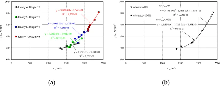
Performed tests showed that density and relative moisture affected the velocity of P-waves in AAC. By performing steps like in point 2.2, at first the correlation curve was determined which presented ultrasound velocity in AAC specimens in air-dry conditions as a function of compressive strength fB. At the beginning, the curve representing the relationship between the average measured

ultrasound velocity as a function of compressive strength fBw of wet AAC, grouping results by AAC

density – Fig. 8a. Higher sound velocity was found in concrete with greater density and compressive strength. Linear dependence, equations of which are illustrated in Fig. 8a, are adequately precise approximations. Fig. 8b illustrates results for compressive strength and corresponding ultrasound velocity of dry AAC (w / wmax = 0%), selected from each density class of

AAC. Then, the relationship cp – fB was calculated with the least square method. For example,

Fig. 8b also shows the relationship of concrete with maximum moisture content (w / wmax = 100%),

obtained similarly.

y = 1,95E-03x - 7,64E-01

R2 _{= 9,32E-01}

y = 3,96E-03x - 3,94E+00

R2 _{= 8,71E-01}

y = 5,06E-03x - 5,57E+00 R2 _{= 7,28E-01}

y = 9,86E-03x - 1,54E+01 R2 _{= 9,72E-01}

0,0 2,0 4,0 6,0 8,0 10,0

0 500 1000 1500 2000 2500

cp, m/s

f

Bw

,

N

/m

m

2

density 400 kg/m^3

density 500 kg/m^3

density 600 kg/m^3

density 700 kg/m^3

y = 5,73E-06x2 _{- 1,46E-02x + 1,03E+01}

R2 _{= 9,98E-01}

y = 6,15E-06x2 _{- 1,72E-02x + 1,39E+01}

R2 _{= 9,84E-01}

0,0 2,0 4,0 6,0 8,0 10,0

0 500 1000 1500 2000 2500

cp, m/s

f

Bw

,

N

/m

m

2

w/wmax=0%

w/wmax=100%

w/wmax=100%

w/wmax=0

(

a

)

(

b

)

Figure 8. Results from P-waves velocity testing: (a) compressive strength of AAC including density classes, (b) AAC strength in wet concrete – fBw and totally dry concrete –fB

For concrete with moisture content w / wmax= 0%, the following empirical relationship was

obtained:

( )

( )

a

fB= p + p+ → B=  p +  p+

− −

,

when

s m 2379 s

m

1847 c_p .

(20)

The curve (20) covers results from testing all densities of AAC, where the obtained coefficient of correlation is R2 _{= 0.98.}

3.3. Calibrating a curve in moisture conditions

including all moisture levels w/wmax and densities, was found with the least square method – Fig. 9a.

The equation of the common curve was:

( )

( )

a

fBw= w p + w p+ w→ Bw=  − p −  − p+ when

s m 2379 s

m

1315 c_p . (21)

Then, equations for individual curves were developed with reference to AAC density. Test results are presented in Table 10. The obtained coefficient values were compared to coefficients aw,

bw and cw for the common curve, and then plotted to the graph Fig. 9b.

y = 5,33E-06x2 _{- 1,39E-02x + 1,09E+01}

R2 _{= 9,67E-01}

0,0 2,0 4,0 6,0 8,0 10,0

0 500 1000 1500 2000 2500

cp, m/s

f Bw , N /m m 2 w/wmax=0% w/wmax=10% w/wmax=23% w/wmax=33% w/wmax=67% w/wmax=100%

a/aw = 1,9852x2 - 1,8865x + 1,0528

R2

= 0,9575

b/bw = 2,771x 2

- 2,5602x + 1,0269 R2

= 0,9739

c/cw = 2,8933x 2

- 2,5613x + 0,9445

R2 = 0,9825 0,0 0,2 0,4 0,6 0,8 1,0 1,2

0,0 0,1 0,2 0,3 0,4 0,5 0,6 0,7 0,8 0,9 1,0

w/wmax a/ aw , b/ bw , c

/cw a/aw

b/bw c/cw Wielom. (a/aw) Wielom. (b/bw) Wielom. (c/cw)

(

a

)

(

b

)

Figure 9. Results from ultrasound velocity testing: (a) common curve fBw–cp for all AAC densities

and moisture levels, (b) equations for curve coefficients at varying moisture content in AAC fBw

Table 10. Comparison of coefficients and equations of empirical curves

w/wmax Curve coefficient R2 Curve equation

a b c

0 _5.73×10-6 _-1.46×10-2 _10.30 0.99 fBw=5,7310−6

( )

0.1 _4.37×10-6 _-1.02×10-2 _7.56 0.97 f_Bw=4,3710 6

( )

−

0.23 _4.22×10-6 _-9.19×10-3 _6.35 0.99 422 10

( )

3 2 6 , c , c ,

fBw=  − p −  − p+

0.33 _3.33×10-6 _-6.21×10-3 _3.88 0.98 f_Bw=3,3310 6

( )

−

0.67 _3.59×10-6 _-7.75×10-3 _5.84 0.95 359 10

( )

3 2 6 , c , c ,

fBw=  − p −  − p+

1 _6.15×10-6 _-1.72×10-2 _13.90 0.98 f_Bw=6,1510 6

( )

−

common curve

aw =

5.33·10-6

bw =

-1.39×10-2 cw =

10.90 0.97 533 10

( )

2 2 6 , c , c ,

fBw=  p −  p+

− −

The method of least squares gives the following forms of empirical curves used to determine coefficients of the relationship fBw–cp for AAC with any moisture level and density:

, , w w , w w , a a m ax m ax w 05 1 89 1 99 1 2 + −      

= R2 _{= 0.96, (22)}

, , w w , w w , b b m ax m ax w 03 1 56 2 77 2 2 + −      

= R2 _{= 0.97, (23)}

, , w w , w w , c c m ax m ax w 94 0 56 2 89 2 2 + −      

Calculated coefficients a, b and c should be put into the equation:

( )

a

fBw= p 2+ p+ , when

s m 2379 s

m

1315 c_p . (25)

which gives the general form of the basic curve for AAC. In practice, ultrasonic testing should be associated with destructive tests for graduation. In this case, further steps can follow rules specified in the European standard EN 13791 [30] for standard concrete.

4. Procedure algorithm for determining characteristic compressive strength of masonry

Proposed empirical procedure for determining characteristic compressive strength of masonry with semi-destructive and non-destructive techniques can be described with the following steps shown in Table 11.

Table 11. Procedure algorithm for determining characteristic compressive strength of masonry with semi-destructive and non-destructive techniques

Step

Description

Semi-destructive technique Reference Non-destructive (ultrasonic)

technique Reference

1 2 3 4 5

1

Determining moisture content by weight w in AAC at the tested

(in-situ) point

equation (16)

Determining moisture content by weight w in AAC at the tested

point

equation (16)

2 Calculating maximum moisture content wmax in AAC

equation (17)

Calculating maximum moisture content wmax in AAC

equation (17)

3

Drilling specimens from AAC, drying them until constant weight

and calculating density ρ

--

Determining P-waves velocity (cp = L/t,) using the transmission method after measuring the path

length L and time t.

--

4 Calculating coefficients a and b of the empirical curve

equation (14) equation

(15)

Calculating coefficients a, b and c

of the empirical curve

equation (22) equation

(23) equation

(24)

5 Calculating the correction factor Δb

equation (13)

Calculating compressive strength of AAC fBw acc. to the

curve

equation (25)

6

Performing destructive tests and determining compressive strength

of dry AAC fc

--

Graduating the curve according to

the standard EN 13791:2008

--

7 Calculating compressive strength

fB acc. to the corrected curve

equation (13)

Calculating compressive strength of AAC fBw acc. to the

graduated curve

--

8

Calculating compressive strength

fBw depending on moisture content

in AAC

equation (18) equation

(19)

Calculating characteristic compressive strength of AAC

masonry

equation (1)

9

Calculating characteristic compressive strength fk of AAC

masonry

equation (1)

5. Conclusions

density of AAC, compressive strength determined at specific volumes and slenderness was found to be similar to the strength of standard specimens. The greatest strength was found in specimens with the smallest volume. And compressive strength of specimens with the greatest volume was much lower than in case of standard cube specimens with dimensions of 100×100×100 mm.

Maximum moisture content is increasing reversely proportional to AAC density, and moisture significantly reduces strength with reference to the strength of AAC tested in air-dry conditions. The greatest 30% reduction in compressive strength was observed at moisture content w = 0 – 30%. Higher moisture levels caused a drop in strength by 10%. AAC moisture coefficient ηw = 0.8

recommended by the standard PN-EN 772-1 may give dangerously overestimated strength of masonry with moisture content w > 20%.

The non-destructive ultrasonic testing demonstrates the profound effect of density and moisture. An increase in P-waves velocity was proportional to density of AAC (maximum velocity was 2379 m/s in concrete with density of 700 kg/m3_{, minimum velocity was 1847 m/s in concrete}

with density of 400 kg/m3_{. Increasing density of AAC caused a significant reduction of the velocity.}

According to general rules of using non-destructive techniques, the established correlation curve with coefficients determined by density can be applied providing the adequate graduation which includes results from non-destructive testing.

Author Contributions:Conceptualization, R.J. and Ł.D.; methodology, R.J. and W.M; validation, R.J..; formal analysis, R.J snd W.M.; investigation, R.J., Ł.D and W.M; writing—original draft preparation, R.J.; writing—review and editing, R.J. Ł. D.; visualization, R.J. and W.M.; supervision, R.J and Ł.D.

Acknowledgements: Authors would like to express particular thanks to Solbet Sp. z o.o. Company for its technical support and supply of materials used during the research works.

Conflicts of Interest: The authors declare no conflict of interest.

References

1. Suprenant, B.A.; Schuller, M. P.: Nondestructive Evaluation & Testing of Masonry Structures. Hanley Wood Inc., USA,1994, ISBN 978-0924659577.

2. Noland, J.; Atkinson, R.; Baur, J. An investigation into methods of nondestructive evaluation of masonry structures. National Science Fundation. National Technical Information Service report No. PB 82218074. 1982.

3. Schuller, M.P. Nondestructive testing and damage assessment of masonry structures. 2006, NSF/FILEM Workshop. In-Situ Evaluation of Historic Wood and Masonry Structures, Jully 10-16, 2006, Prague, Czech Republic, pp. 67 – 86.

4. McCann, D.M.; Forde, M.C. Review of NDT methods in the assessment of concrete and masonry structures. NDT E Int. 2001, 34, 71–84. https://doi.org/10.1016/S0963-8695(00)00032-3.

5. Łątka, D.; Matysek P. The estimation of compressive stress level in brick masonry using the flat-jack method. Procedia Engineering2017, 193, pp. 266-272, https://doi.org/10.1016/j.proeng.2017.06.213.

6. Matysek, P. Compressive strength of brick masonry in existing buildings – research on samples cut from the structures. In Brick and Block Masonry – Trends, Innovations and Challenges, 3rd ed; Modena, da Porto & Valluzzi, Eds; © 2016 Taylor & Francis Group, Great Britain, London, ISBN 978-1-138-02999-6, pp. 1741-1747.

7. PN-EN 1996-1-1:2010+A1:2013-05P, Eurocode 6: Design of Masonry Structures. Part 1-1: General rules for reinforced and unreinforced masonry structures. (In Polish)

8. EN 772-1:2011 Methods of test for masonry units. Determination of compressive strength. 9. Neville, A.M. Properties of Concrete, 5th edition, Pearson Education Limited, 2011, Essex, England.

10. Kadir, K.; Celik, A. O.; Tuncan, M.; Tuncan, A. The Effect of Diameter and Length-to-Diameter Ratio on the Compressive Strength of Concrete Cores, Proceedings of International Scientific Conference People, Buildings and Environment 2, pp. 219-229. ISSN: 1805-6784.

11. Bartlett, F. M.; Macgregor, J. G. Effect of Core Diameter on Concrete Core Strengths, 1994, ACI Materials Journal, 91(5, Sept.-Oct.), pp. 460-470.

13. Gębarowski; P.; Łaskawiec, K. Correlations between physicochemical properties and AAC porosity structure, Materiały Budowlane 2015, 11, pp. 214-216. (in Polish)

14. Zapotoczna-Sytek, G.; Balkovic, S. Autoclaved Areated Concrete. Technology, properties, application. Wydawnictwo Naukowe PWN, Warszawa 2013. (in-Polish)

15. Mazur, W.; Drobiec, Ł.; Jasiński, R. Effects of specimen dimensions and shape on compressive strength of specific autoclaved aerated concrete. Ce/Pepers, Volume 2, Issue 4, 2018, pp. 541-556. https://doi.org/10.1002/cepa.837.

16. EN 771-4:2011 Specification for masonry units - Part 4: Autoclaved aerated concrete masonry units 17. Weibull, W. A Statistical Theory of Strength of Materials. Ingvetenskaps Handl. 1939.

18. Weibull, W. A statistical distribution function of wide applicability.Journal of Applied Mechanics, 1951, 18, 1951, pp. 293 – 297.

19. Bartlett, F. M.; Macgregor, J. G. Effect of Moisture Condition on Concrete Core Strengths, 1993, ACI Materials Journal 91(3, May-June), pp. 227-236.

20. Jasiński, R. Determination of AAC masonry compressive strength by semi destructive method. Nondestructive testing and diagnostics, 2018, 3, pp. 81 – 85. https://doi: 10.26357/BNiD.2018.029.

21. Matauschek, J.; Einführun in die Ultraschalltechnik. Berlin, Verlag Technik. 1957.

22. Stawiski, B.; Kania, T. Determination of the Influence of Cylindrical Samples Dimensions on the Evaluation of Concrete and Wall Mortar Strength Using Ultrasound Method. Procedia Engineering2013,

57, pp. 1078-1085, https://doi.org/10.1016/j.proeng.2013.04.136.

23. Roland, J.; Atkinson, R.; Kingsley, G.; Schuller, M. Nondestructive evaluation of masonry structures. National Science Fundation. Project No. ECE-8315924. 1990.

24. Stawski, B. Ultarsonic testing of concrete and mortar using point probes. Scientific Papers of the Institute of Building Engineering of the Wrocław University of Technology. No. 92. Monographs. No. 39. 2009 (in Polish).

25. Drobiec, Ł.; Jasiński, R.; Piekarczyk, A. Diagnostic testing of reinforced concrete structures. Methodology, field

tests, laboratory tests of concrete and steel. Wydawnictwo Naukowe PWN, Warszawa 2013. (in-Polish)

26. Haach, V.G.; Ramirez, F.C. Qualitative assessment of concrete by ultrasound tomography. Constr. Build. Mater. 2016, 119, 61–70. https://doi.org/10.1016/j.conbuildmat.2016.05.056.

27. Schabowicz, K. Ultrasonic tomography—The latest nondestructive technique for testing concrete members — Description, test methodology, application example. Arch. Civ. Mech. Eng. 2014, 14, 295–303. https://doi.org/10.1016/j.acme.2013.10.006.

28. Rucka, M.; Lachowicz, J.; Zielińska, M. GPR investigation of the strengthening system of a historic masonry tower. J. Appl. Geophys. 2016, 131, 94–102. https://doi.org/10.1016/j.jappgeo.2016.05.014.

29. Zielińska, M.; Rucka, M. Non-Destructive Assessment of Masonry Pillars using Ultrasonic Tomography. Materials. 2018, 11, 2543; https://doi:10.3390/ma11122543.