Initial Results on Deep Learning-Based Pilot Contamination Mitigation in Massive MIMO Systems

Initial Results on Deep Learning-based Pilot Contamination Mitigation in Massive

MIMO Systems

Felipe Augusto P. de Figueiredo

Department of Information Technology, Ghent University - Gent - Belgium [email protected]

Abstract

In this brief letter we report our initial results on the application of deep-learning to the massive MIMO channel estimation challenge. We show that it is possible to estimate wireless channels and that the possibility of mitigating pilot-contamination with deep-learning is possible given that the leaning model underwent an extensive training-phase and that it has been presented with a large number of different channel conditions.

Keywords_​: massive MIMO; pilot contamination; deep learning; machine learning.

Introduction

Pilot contamination occurs when two terminals use the same pilot sequence (also known as reference signal) at the same time/frequency resource. It can be suppressed by using different pilots in adjacent cells - for example, by having a large number of pilots sequences and switching randomly between them. Conventional systems can afford to have many more pilot sequences than active terminals, which makes the risk of pilot "collision" rather small. In contrast, Massive MIMO cannot afford that since it is supposed to have 20-40 times more active terminals on the same time/frequency resource than conventional systems. In other words, if a system has 30x more terminals the pilot contamination will be 30x more severe [1, 2].

Therefore, techniques to mitigate such problem become of utter importance in Massive MIMO systems.

This work presents our initial results in deep learning for channel estimation, pilot contamination mitigation and symbol detection. It demonstrates that DNNs have the ability to learn and analyze the characteristics of wireless channels in massive MIMO systems.

Problem definition

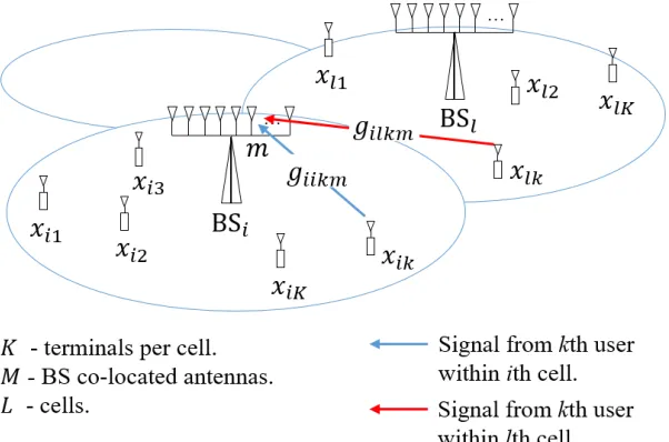
We assume as illustrated in Fig. 1 a multi-cell system with L cells, where each cell has a BS at its center with _​M co-located antenna elements and _​K randomly located single antenna users. We also assume _​flat Rayleigh fading channels being independent across users and antennas. Let g_ilkm represent the complex gain of the channel from the _​k_​th user in the _​l_​th cell to the _​m_​th BS antenna in the i_​th cell. We can write_​ g_iikm =

_√

β_ilk h_iikm where β_ilk is the large-scale coefficient encompassing both path loss and log-normal shadowing. We assume the same large-scale coefficient value for all BS colocated antennas, and h_ilkm is the small-scale coefficient with a circularly-symmetric complex normal distribution _​CN_​(0,1). We assume that the large-scale fading coefficients do not depend on the antenna index _​mof a given BS because

typically, the distance between a user and a BS is significantly larger than the distance between the BS antennas. The wireless channels are considered static during the channel coherence time, _​τ_​, (i.e., channel estimates are effective only in this time interval) and independent across users and antennas.

Figure 1_​ - Problem definition.

Uplink Training

Each user transmits an uplink training sequence so that the user serving BS can estimate the channels per antenna and subsequently detect the transmitted user data. We assume that users in different cells transmit data at the same time-frequency resource (a typical scenario in massive MIMO) and that the pilot reuse factor is one, the worst possible use case scenario. As all BSs reuse the same set of pilots and transmit at the same time-frequency resource, the pilot contamination problem arises, consequently, all the other BSs will also receive the pilots sent by users being served by other BSs, limiting the quality of the channel estimation.

The pilot signals of K users are represented by a N x K matrix S_​ of the form_​S = [s₁, s₂, …, s_K], where _​N is the length of the pilot sequences. Each pilot sequence is of the form s_k = [

, , ..., . The pilot matrix,_​S_​, exhibits orthogonal property = N . Within a cell,

s0

k s1k sNk−1 ]

T _SH_{S I}

K

the K terminals always use orthogonal pilot sequences to eliminate intra-cell pilot interference (τ ≥ K)_​.

The received uplink training sequences at the _​i_​th BS can be represented as a _​M x N

As can be seen by analysing the LS equation above, we notice that the received pilot signal is contaminated with transmissions from terminals in other cells reusing the same pilot sequence.

The Least Squares (LS) estimator is given by the equation below_​.

As can be seen by analysing the equation above, the channel estimate of g_iik is contaminated by the channels of other cells reusing the same pilot sequence.

Deep Learning Methods

neurons, which need to be optimized before the online deployment. The optimal weights are usually learned on a training set, with known desired outputs, i.e., labels.

Precoding techniques

Maximum ratio transmission (MRT, also known as conjugate beamforming) is an approach that focuses transmitted signal power to the location of desired terminal, while not considering its impact on interference at rest of the terminals. MRT is therefore an SNR-maximizing technique. On the other hand, zero-forcing (ZF) design places nulls at the location of the rest of the terminals to minimize interference at those terminals. However, it transmits the signal in all other directions, a fraction of which may be received by the desired terminal. In general, MRT is preferable for noise-dominated regime, while ZF is preferred for high-SNR regime where interference dominates the SINR.

Downlink transmission

During downlink transmission, pilot contamination adversely affects the precoding weight vectors for the kth terminal. In case of MRT precoding, the BS uses the channel estimates to focus signal energy at the location of the kth terminal. Due to the contaminated channel estimates, some of the transmit power leaks towards the kth terminals in other cells, attenuating the signal power at the desired terminal. Moreover, this leakage appears as focused interference at these terminals, decreasing their SINR. Thus, the impact of pilot contamination on downlink data transmission with MRT precoding is twofold: the signal power lost for desired terminal appears as sharply focused interference at other terminals that reuse the same pilot sequence.

Remarks

1. MMSE Estimation

The Bayesian MMSE estimator is optimal if the channel statistics are known [5]-[9], while the minimum variance unbiased (MVU) estimator is applied otherwise [5]. If z_ik , g_kii are jointly Gaussian, then the linear MMSE estimator and the optimal (Bayesian) MMSE estimator coincide.

The estimator in Theorem 3.1 is therefore sometimes called the linear MMSE (LMMSE) estimator. However, we prefer to use the MMSE notion to make it clear that one cannot further reduce the MSE by using a non-linear estimator [10].

2. Large Scale fading

The measurements in [11] suggest that the large-scale fading is constant for a time interval around 100 times longer than the coherence time. The measurements in [12] suggest roughly two orders of magnitude slower variations.

According to [13] in a mobile scenario where Bs = 10 MHz, Ts = 0.5 s, Bc = 200 KHz and Tc = 1 ms, the number of coherence blocks where the large-scale fading can be considered static is equal to 25000.

Performance Assessment

In this section we highlight a few metrics and points to evaluation the performance of the deep learning-based pilot-contamination mitigation schemes.

● Flat Rayleigh Fading Channel Model_​: initially, we will adopt this model once it is simple and will give us a better/faster insight of the possible results of applying deep learning to channel estimation and pilot contamination problems.

● Frequency Selective Channel Model

● Realistic Channel Models

● Comparison of MSE and BER with LS/MMSE/Proposed

● Impact of the number of pilots on the performance

● Impact of the number of hidden layers on the performance

● Assess the performance with different deep learning architectures? ○ Feedforward Neural Networks

○ Convolutional Neural Networks ○ Recursive Neural Networks ○ Recurrent Neural Networks

● How long does it take to train? Relation between number of training vectors and observed performance.

● It might not be necessary to consider other users’ signals as interference, i.e., we could try to estimate all the other channels at the same time based on the observation we have. Current techniques focus only on estimating the channel from the k-th user in the i-th cell and consider the other channels as interference.

Realistic channel models

In this section we list some channel models that represent realistic representation of wireless channels.

Geometry-based stochastic models (GSCM)

○

WINNER II Channel Model for Communications System Toolbox

■ Widely used for its scalability and reasonable low complexity with respect to Ray Tracing.

■ https://nl.mathworks.com/matlabcentral/fileexchange/59690-winner-ii-cha nnel-model-for-communications-system-toolbox

■ The channel model supports:

● RF frequencies up to 6 GHz, and signal bandwidths up to 100 MHz.

● Line-of-sight (LOS) and non-LOS propagation. ● 12 indoor and outdoor propagation scenarios.

● Arbitrarily large antenna arrays (for massive MIMO applications). ● Isotropic, dipole and user-defined antenna element patterns ● A variety of antenna array types (linear, circular, and user-defined)

○

Quadriga Channel Model

■ Quadriga channel model is provided by the Fraunhofer Institute.

■ Extension of WINNER II and WINNER+ models with full 3D characterization of the channel, including a geometric polarization model. ■ Quasi-deterministic radio channel generator

■ The model supports:

● RF frequencies from 500 MHz to 100 GHz, _​and signal bandwidths up to _​100 MHz (from version 2 onwards).

● Line-of-sight (LOS) and non-LOS propagation.

● 3D spatial consistency of large and small-scale fading based on the sum-of-sinusoids method.

● Multi-frequency simulations (supporting carrier aggregation and functional split).

● Scalability from a single input single output (SISO) or

multiple-input multiple-output (MIMO) link to a multi-link MIMO scenario.

● Support of multi-antenna technologies, polarization, multi-user, multi-cell, and multi-hop networks

■ http://quadriga-channel-model.de/

Training Scenarios

The training scenarios are based on the ones employed in [4]. In [4], we adopt a typical multi-cell structure as the one shown in Fig. 1 with L = 7 cells, i.e., one central cell surrounded by 6 other cells, K = 10 users in each cell, the frequency reuse factor of 1 and N = K pilot symbols. We consider two different types of setups for setting the large-scale fading coefficients {β_ilk }:

Fixed values

For the fixed case, we set β_iik = 1 and β_ilk = a, l=/i , where _​a represents the cross-cell interference level. The value selected for “_​a” in the fixed case is 0.05 and it is chosen so that there is moderate cross-cell interference level from users being served by other BSs, i.e., not being served by the central cell.

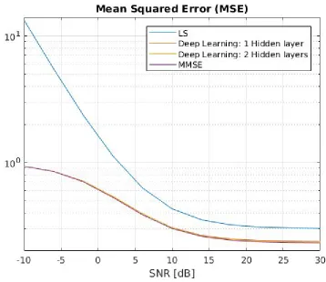
Figure 1 - Scenario 1: Channel Estimation MSE versus uplink pilot power.

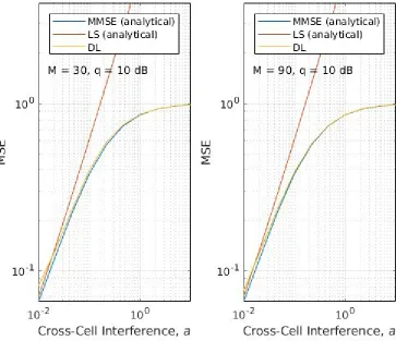
● 2nd scenario: Channel estimation MSE versus cross-cell interference level_​: ○ M = 30,_​ q_​ = 10 dB, _​a_​ = 1e-2 up to 1.

Figure 2 - Scenario 2: Channel estimation MSE versus cross-cell interference level

Conclusions

In this work we have shown that it is possible to estimate wireless channels and that the possibility of mitigating pilot-contamination with deep-learning is possible given that the leaning model underwent an extensive training-phase and that it has been presented with a large number of different channel conditions.

References

[1] Emil Björnson, Erik G. Larsson, and Mérouane Debbah, “Massive MIMO for Maximal Spectral Efficiency: How Many Users and Pilots Should Be Allocated?”,_​IEEE Transactions on

Wireless Communications_​, vol. 15, no. 2, Feb. 2016.

[2] Olakunle Elijah, Chee Yen Leow, Tharek Abdul Rahman, Solomon Nunoo, and Solomon Zakwoi Iliya, “A Comprehensive Survey of Pilot Contamination in Massive MIMO—5G System”, IEEE Communications Surveys & Tutorials, vol. 18, no. 2, 2016.

[4] Felipe A. P. de Figueiredo et. al, “Channel Estimation for Massive MIMO TDD Systems Assuming Pilot Contamination and Flat Fading”, EURASIP Journal on Wireless Communications and Networkin_​g, vol. 2018, no. 14, Jan. 2018.

[5] S. Kay, Fundamentals of Statistical Signal Processing: Estimation Theory. Prentice Hall, 1993.

[6] J. Kotecha and A. Sayeed, “Transmit signal design for optimal estimation of correlated MIMO channels,” IEEE Trans. Signal Process., vol. 52, no. 2, pp. 546–557, 2004.

[7] Y. Liu, T. Wong, and W. Hager, “Training signal design for estimation of correlated MIMO channels with colored interference,” IEEE Trans. Signal Process., vol. 55, no. 4, pp. 1486–1497, 2007.

[8] E. Bjornson and B. Ottersten, “A framework for training-based estimation in arbitrarily correlated Rician MIMO channels with Rician disturbance,” IEEE Trans. Signal Process., vol. 58, no. 3, pp. 1807– 1820, 2010.

[9] N. Shariati, J. Wang, and M. Bengtsson, “Robust training sequence design for correlated MIMO channel estimation,” IEEE Trans. Signal Process., vol. 62, no. 1, pp. 107–120, 2014. [10] Emil Björnson, Jakob Hoydis and Luca Sanguinetti (2017), “Massive MIMO Networks: Spectral, Energy, and Hardware Efficiency”, Foundations and Trends in Signal Processing: Vol. 11, No. 3-4, pp 154–655. DOI: 10.1561/2000000093.

[11] Viering, I., H. Hofstetter, and W. Utschick. 2002. “Spatial long term variations in urban, rural and indoor environments”. In: COST273 5th Meeting, Lisbon, Portugal.

[12] I. Viering, H. Hofstetter, and W. Utschick, “Spatial long-term variations in urban, rural and indoor environments,” in the 5th Meeting of COST273, Lisbon, Portugal, 2002.

[13] Emil Bjornson, Luca Sanguinetti, Merouane Debbah, “Massive MIMO with Imperfect Channel Covariance Information”, 2017.