A Comparative Analysis of Clustering Algorithms and Recent Developments

Volume 8, No. 3, March – April 2017

International Journal of Advanced Research in Computer Science RESEARCH PAPER

Available Online at www.ijarcs.info

A Comparative Analysis of Clustering Algorithms and Recent Developments

Sandeep Mukherjee

Department of Computer Science and Engineering Birla Institute of Technology, Mesra, Kolkata Campus,

Kolkata, India

Ambar Dutta

Department of Computer Science and Engineering Birla Institute of Technology, Mesra, Kolkata Campus

Kolkata, India

Abstract:Clustering is very central to the concept of data mining applications and data analysis. It is a very desirable capability to be able to identify regions of highly co-related objects as their count becomes very high and at the same time the data sets enlarge and changes in their properties and relationships among the datasets also altered. It is important to note that the concept of clustering is fundamentally a partitioning of some or many objects based on a set of rules. In the literature, a considerable number of clustering algorithms are available which are classified into various categories. In this paper, an attempt is made to perform a comparative analysis of some state-of-the-art clustering algorithms based on different parameters. At the end, some recent advances of clustering algorithms are also highlighted.

Keywords:Data mining; clustering; comparison; evaluation parameters; recent advances

I. INTRODUCTION

Data mining is a process of extracting implicit, previously unknown, interesting and useful information from huge data. Data mining is also synonymous to Knowledge discovery, which is a multistage process including pre-processing, data mining process and post-processing. Pre-processing is extraction, cleaning and trans-formation of data. In data mining process various algorithms are applied to generate hidden knowledge. Mining results are evaluated as per requirement of the user and knowledge of domain. There are various data mining techniques – Classification, Clustering, Association Rule Mining, Sequential Pattern Mining, Outlier Analysis etc. The techniques used is dependent on user requirement and data type.

The present paper focuses on Clustering and various major techniques associated with it. Clustering can formally be defined as the process of forming a group of a set of physical or abstract objects into classes of objects that are similar to each other. In clustering it is desired that a set of objects clustered or grouped together should exhibit similarity to a great extent, whereas those belonging to different cluster should exhibit discerning degree of dissimilarity. In simple terms - High intra-cluster similarity and low inter-cluster similarity should exist amongst object points. There are several Applications of Cluster Analysis. In the field of pattern recognition, image processing, market research and data analysis, clustering analysis has its applications. Marketers can identify the specific groups in their customer base with the assistance of Clustering technique. Depending on the purchasing patterns the marketers can characterize the specific customer groups. Plant and animal taxonomies can be derived in the field of biology. This technique can be used to categorize genes which are alike in functionalities and develop some idea about structures inherent to populations. Also in the field of GIS - identification of groups of houses can be identified by house type in a city, its value, and the geographic location, is possible. With the help of clustering documents from the web can be classified for information and knowledge discovery. Clustering can also be used for detection of outlier applications and credit card fraud detection [1].

The rest of the paper is summarized as follows. Section II deals with the detailed classification of clustering algorithms which is followed by a brief description of a few algorithms

in each category in section III. Section IV presents an exhaustive comparative analysis of clustering algorithms presented in Section III. Section V describes some of the recent developments in clustering algorithms. Finally, Section VI provides the concluding remarks.

II. CLASSIFICATION OF CLUSTERING ALGORITHMS

Several classifications of clustering algorithms exist for the reason the idea of a ‘cluster’ has not been clearly stated. As a result many clustering methods have been proposed – each of which have a different notion. The classification of clustering algorithms into two major groups – the hierarchical and partitioning, was suggested by Farley and Raftery in 1998 [2]. Three more groups – density-based, grid-based and model based categorization was first suggested by Han and Kamber [1].

A. Partition-based Methods

In a partitioning method if k be the number of partitions of the data and n be the number of objects and a cluster is represented by a partition and k <= n. data is di-vided by the method into k groups. With each group having a minimum of 1(one) object. Partitioning methods carry out 1-level of partitioning on the data set. Exclusive cluster separation method is carried out so that each object is associated with exactly 1(one) group/cluster.

Usually the partitioning methods adopt a distance based approach. For a particular value of ‘k’ (denoting the number of partitions), an initial partitioning is done by the method employed. Thereafter the process is refined by iterative use of the technique. This is done by moving the objects of 1(one) group to another at each iteration. A greedy approach like the k-means or k-medoids is adopted by most techniques. These are essentially heuristic and improve the results i.e. the quality of clustering upon successive iterations and an optimum result is obtained locally. This approach produces very good result for spherical shaped clusters, when the size of database ranges from small to moderate. Important methods are k-means, k-medoids.

B. Hierarchical Methods

merged till the algorithm terminates. This is a bottom–up approach.

The objects from the same classes are considered in the second approach – the divisive approach. A cluster is split into smaller clusters till each individual objects are assigned a single cluster or till the algorithm terminates. It is a top-down approach. Hierarchical methods are further classified into two sub-categories – (i) agglomerative and (ii) divisive. Agglomerative clustering begins by considering each object as individual cluster and by an iterative merging process progressively larger clusters are found. This is done till all elements are grouped into a single monolithic and some termination condition is attained. The monolithic structure may then be considered to be a root of the cluster hierarchy. Two clusters which are closest are merged on the basis of some similarity measure – it may be the nearest distance between the two. The strategy employed in Divisive clustering is just the opposite to that of Agglomerative clustering – it top-down instead of bottom-up. At the start all object points are grouped into a single big cluster. Smaller sub-clusters are produced from bigger clusters by division. Several levels of sub-clusters may be produced from bigger clusters till no further sub-division is possible – either the cluster becomes a single element one or the intra-cluster elements exhibit extreme similarity. Depending on the degree of linkage between the individual elements of clusters, the hierarchical method can be further divided into (i) single-link, (ii) complete-link and (iii) average-link [3]. Important method in this category is BIRCH, CURE etc.

C. Density based Methods

Distance between objects is the primary consideration of the most partitioning method. For such techniques discovering only spherical shaped clustering is easier. These techniques find it hard to discover arbitrary shaped clusters. Idea of density has assisted the development of other clustering techniques. Here the main idea is to continue the growth of a given cluster till the density value reaches a threshold in the neighborhood. The method can then be used to eliminate noise and abnormal or outlier values and find the arbitrarily shaped clusters. These methods help in dividing the input values into a hierarchy of clusters or a number of distinct clusters. Important methods are: DBSCAN, OPTICS, DENCLUE etc.

D. Grid-based Methods

This method segregate the object space into a grid like collection of structures of a definite number of cells. The grid is the scene of the clustering operations. This approach has a very quick processing time. The processing time primarily depends on the number of cells at every dimension of the grid. The processing time does not de-pend on the number of data objects. Important method is: STING.

E. Model Based Methods

An optimum fit between a given dataset and a mathematical model is attempted in this approach. General clustering methods identifies object groups but this approach also finds typical description for the groups. A class or a concept is represented by each of the groups. ‘Decision trees’ and ‘Neural Network’ are two very important application areas. Important methods are: COBWEB, Expectation Maximization (EM) Algorithm.

III. DESCRIPTION OF SOME IMPORTANT ALGORITHMS

A. K-Means

There are ‘n’ data elements in the Dataset D. By means of partitioning methods the ‘n’ data elements of the Data set D are grouped into ‘k’ disjoint clusters – C1, C2, ... CK. The

goal of the objective function is to maintain strong inter-cluster similarity and weak intra-cluster similarity in centroid based algorithms. The centre of the cluster is meant by the centroid. Mean or medoid of the points belonging to the cluster signifies the centroid of that cluster. The value of the intra-cluster variation is an indication of the cluster quality. It is measured as the sum of the squared error between p and Ci.

B. K-Medoids

The output of k-means algorithm is affected by the presence of outliers. These objects are located far away from the purported data clusters. They can significantly alter the mean of the cluster to which they are assigned. To overcome this shortcoming a value of 1(one) suitable cluster member is chosen as representative of the cluster. This is done in case of all the clusters. Thus here the k-means is modified to eliminate/reduce such effect of the outliers – actual objects can be chosen from the datasets to represent the clusters to which it bears the maximum similarity. The partitioning of the clusters is done by minimizing the summation of the distance between the two objects and the representing object of the cluster where the object belongs. Thus n objects are grouped into k clusters. This forms the essence of k-medoids method. When k=1, the exact median can be found to be in O(n2

C. BIRCH

) time. However when k is a normal positive number, the k-medoid problem is considered to be an NP-hard problem.

BIRCH is the acronym for Balanced Iterative Reducing and Clustering using Hierarchies[4]. It is a 2-stage process in which Hierarchical partitioning is used at the initial micro-clustering stage and thereafter in the second phase of macro-clustering by iterative partitioning. In this method a huge amount of numeric data can be clustered. The two major problems of agglomerative clustering are – i) scalability and ii) inability to undo actions that have been done in the previous steps. These have been overcome in BIRCH. In BIRCH a cluster is summarized by using the notions of clustering feature and cluster hierarchy is represented by the clustering feature (CF) tree. Good speed and scalability can be attained even in streaming databases by using the aforestated structures. The clustering technique is also made effective for handling dynamic and incremental clustering of the streaming objects. There are two important phases of BIRCH.

PHASE I: at first an in-memory CF-Tree is built after the algorithm scans the database. This may be considered as a multilevel compression of data, where the natural clustering structure of the data remains unaltered. PHASE II: The leaf-nodes of the CF tree are clustered by selective application of the clustering algorithm. Thus dense clusters become grouped into larger clusters and the spare clusters are considered as outliers and are removed.

For n objects the time-complexity has been observed to be O(n). it has been empirically observed that a considering the number of elements to be clustered the BIRCH has been linearly scalable and the clustering quality is good.

D. DBSCAN

E. OPTICS

In this technique [5] no explicit data set clustering is produced. A cluster ordering is produced as output instead and a linear list of all objects under scrutiny is produced and a density based cluster structure of the data set is produced, in this method. In the cluster ordering those objects which are in a denser cluster are listed closer to each other. This ordering of objects belong to is found to be the same to the density-based clustering that is calculated from a varied range of parameter settings. N specific density threshold is required to be stated by the user in OPTICS. Basic clustering in-formation can be extracted – like cluster centres or clusters of arbitrary shapes. The cluster ordering also helps in determining the fundamental structuring of the clustering. For simultaneous construction of different clusters the object points are processed in a definite order. This definite order helps in selection of a density reachable object with the lowest ε value so that the clusters having higher density (lower ε) will be processed first.

The OPTICS algorithm requires two important information for each object, based on this idea:

• The first is that the smallest value ε is such that there are at least MinPts number of objects in the neighborhood of p

• The second is that the minimum value of the radius for which p is able to be ‘density reachable’ from ‘q’, then that value is termed as the reachability distance.

With relation to many different core objects an object p may have several reachability distances if an object ‘p’ may be directly reachable from multiple core objects. The least reachability distance of p is most important as it gives the shortest path with which p has a connection to a dense cluster.

OPTICS clustering technique saves ‘core distance’ and an appropriate ‘reachability distance’ for each object point of the data cluster and also finds an ordering for the entire set of objects of the database..

F. STING

It is an acronym for STatistical INformation Grid [6]. In STING the spatial area is partitioned into rectangular cells in this typical multi-resolution approach to clustering. Various levels of rectangular cells are there, which synchronizes with various resolution levels. A hierarchical structure is formed by these cells. A number of cells at the lower level is formed by partitioning each cell at high level. Pre-computation and storage of statistical information of various attributes of cells of the grid (like – mean, max. and min. values) are done.

In the following manner, using top-down approach and grid-like method the statistical parameters can be utilized. At first a layer is identified within the hierarchical structure. The ‘query-answering’ process is initiated from that layer. This layer usually has a very few cells. A confidence interval or approximate probability interval is calculated which corresponds to how the cell is relevant to the query. The cells which are more relevant are not considered any further. Only the leftover relevant cells are processed at the next lower level. The process continues till the cells of the lowermost level are processed. The areas of the relevant cells satisfying the query are returned at this point of time provided the query specification is satisfied.

G. Expectation Maximization (EM)

This algorithm adjusts and readjusts the object points against the mixture density which is produced by the vector. Thereafter parameter estimates are updated using the readjusted object points. The algorithm proceeds as follows:

1. An initial estimate of the parameter is made. This is done by choosing ‘k’ object points randomly for representing the cluster means or centroids.

2. Parameters are refined in a step-wise manner on the basis of the following steps:

• Expectation step: a cluster Ck is assigned to each object xi having probability j, where p(xi, Ck) = N(mk, Ek(xi)) and the Gaussian distribution is followed with mean, mk, with expectation, Ek.

• Maximization Step: here the model parameters are better estimated or defined by using the probability estimates derived from the Expectation step

This step maximizes the probability of the distribution corresponding to the provided data.

IV. COMPARATIVE ANALYSIS OF ALGORITHMS

This section presents the relative advantages and disadvantages of the above mentioned clustering algorithms. A comparison table (Table – I) is also provided in this paper based on various parameters.

A. K-Means

It is comparatively more scalable and very efficiently processes large data sets. However its application is subject to proper definition of cluster mean. The value of K has to be specified by the user. The algorithm cannot be applied to discover non-convex shaped clusters and also clusters of varying sizes. The Mean value is influenced since the method is sensitive to noise and outlier data points. Also it is not good on overlapping data.

B. K-Medoids

Performance comparatively less affected in the presence of noise and outliers than k-Means. But the algorithm is costlier than the k-Means method. The value of K has to be specified by the user. In presence of large data sets the algorithm scales up poorly.

C. Hierarchical method (Agglomerative/ Divisive)

These algorithms can produce better-quality clusters. However the computational and storage requirements-wise the method is expensive. Also in case of hi-dimensional data and data with hi-level of noise, the finds the merges once made cannot be undone.

D. BIRCH (An instance of Divisive method)

The best possible clusters are derived by making optimum use of the memory at disposal. Good clustering achieved at the initial scan. Subsequent clustering achieved by undertaking further scans result in development of further clusters or improved clusters. In BIRCH a decision is arrived at by not scanning all the data points so the algorithm is local in that sense. Algorithm handles only numeric data. The result depends on the order of the data record.

E. DBSCAN

F. OPTICS

The method overcomes the weakness of DBSCAN in detecting meaningful clusters in data of varying density. However, it is 1.6 times slower than DBSCAN.

G. STING

This Grid-based computation is query independent. Also good quality clusters obtained for noisy data sets. The

method is slower than DBSCAN (though faster than BIRCH).

H. EM

The method is simple and easy to implement. It performs much better on the overlapping data. It converges fast. Though the method implements well by quick convergence, however global optimum may not be achieved. The method is very sensitive to the selection of initial parameters.

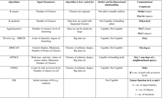
Table I. Comparative Analysisof Clustering Algorithms Based on Various Parameters

Algorithms Input Parameters Algorithm is best suited for Outlier and hi-dimensional

datahandling

Computational

Complexity

K-means Number of Clusters Clusters are separate Not able to handle outliers O(nkt) (time)

O(n+k) (space)

K-medoids Number of Clusters Data Sets are small with

Separated Clusters

Not Capable of handling either

O(k(n-k)2)

Agglomerative Number of clusters/ level of clustering

Data set can be relatively large

Capable, Not Capable O(n2

O(n ) (time)

2_{) (space)}

Divisive eg. – BIRCH Limit of diameter, degree of branching

Big data set Capable, Not Capable O(n)

DBSCAN Clusters Radius, Minimum,

Number of Points in Clusters

Clusters of arbitrary shapes, Big data set

Capable, Not Capable O(n log n)

OPTICS Both max. and min. values of

cluster radius, Minimum Number of Clusters

Clusters of arbitrary shapes, Big data set

Capable of handling both O(n * run-time of ε -neighbourhood query)

STING Count of cells in lowest level,

Number of objects in cell

Clusters of arbitrary shapes, Big data set

Capable, Not Capable O(K)

K is no. of grid-cells at lowest level

EM Initial estimate of Θ (e.g.,

random)

Not Capable Linear function in d, n and t

d = no. of input features,

n = no. of objects,

t = no. of iterations

V. RECENT DEVELOPMENTS OF CLUSTERING ALGORITHMS

The present section highlights some of the recent advances of clustering algorithms which includes the following classifications [7, 8, 9, 10].

A. Fuzzy Clustering

In traditional Clustering approach one object instance strictly belongs to one cluster. This type of clustering is disjointed or hard. Fuzzy Clustering is an extension of this idea and softy clustering principles are followed. Here using a kind of mapping function each pattern is associated with every cluster. In other words each and every cluster is a fuzzy set of all patterns. High degree of confidence in the assignment of patterns to the cluster is indicated by the large value of the membership. A threshold of the membership value is determined for the determination of hard clustering from a fuzzy partition. A popular algorithm is this category is Fuzzy C-Means which performs better than hard K-means algorithm. Most vital problem in Fuzzy Clustering is the construction of membership function.

B. Evolutionary Approaches in Clustering

This approach may be considered to be a general statistical method for a solution to the optimization problem. Evolutionary path may be very suitable as clustering problem on the whole is a problem of optimization. The central idea is

the convergence of a big pool of cluster structures by making use of evolutionary operators, into universally optimal clustering. In chromosome-like abstracts the candidate clustering are encoded. Selection, recombination and mutation are the most frequently and popularly used evolutionary operators. The likelihood of a chromosome serving the next generation is determined by a fitness function evaluated on it. Genetic algorithms are very popularly used in the problems of clustering involving evolutionary technique. With each cluster is associated a fitness value. Larger values of fitness implies that the clustering structure has low value of squared error.

C. Spectral Clustering

The well-known clustering techniques like k-means or EM form clusters having regular geometric shape of convex type. Spectral Clustering is capable of dealing with far greater complexities. The shapes may be arbitrarily non-linear like an intertwined spiral. Areas of application of the various types of the Spectral Clustering Algorithm are i) text mining, ii) Speech Processing and iii) Image Segmentation. Spectral Clustering is a 3 step method – (i) A similarity graph is constructed for all the data prints, (ii) Using the eigenvectors of the graph Laplacian, the clusters of the embedded data points in the space become very apparent, (iii) Finally to partition the embedded points a traditional clustering technique like the k-means is applied.

D. Uncertain Data Clustering

collectable then the uncertainty can be used to improve the results of data mining algorithms. The technique of ‘Uncertain Data Clustering’ is often wrongly confused with ‘Fuzzy Clustering’. In the former case the uncertainty concerns the representation of the clusters. The clustering itself is either probabilistic or deterministic, whereas in the latter case the clusters are deterministic but the membership of objects to the clusters are probabilistic.

Uncertain data clustering has broadly been classified as [11, 12, 13, 14, 15]:

• Mixture modelling algorithms: A good example is EM Algorithm where for modelling uncertain data probabilistic technique is used.

• Density based methods: density based method is used for uncertain data mod-elling like FDBSCAN, FOPTICS etc.

• Partitional method: Lee S. D et. al. [13], Aggarwal C. et. al. [14]) modified K-means algorithm is employed to tackle uncertain data is used.

• High Dimensional Algorithms [15]: This type of data is very sparse which itself is very challenging.

E. Multimedia Clustering

It concerns clustering of feature and semantic spaces and varying levels of granularity. This clustering helps in far more robust and uniform analysis and interpretation of the multimedia objects by carrying out in-depth and complementary clustering at the various levels of the multimedia domain. So clustering of multimedia data is considered to be a very much accepted technique and application. As pre-processing steps of multimedia – a construction of visual dictionary can be done; automatic video structuring and also content summary of the images can be done. In real world applications of multimedia noisy, multi-model high-dimensional data in large scale in encountered. This is a very big challenge. The methods involved involving the afore-mentioned challenges depend very much on the procedures followed in processing real world application. Clustering techniques can be applied to a varied number of image data. These include image segmentation, photo album event recognition, face clustering and annotation, video story clustering, music-summarization, video summarization and video event detection etc [16, 17, 18, 19].

VI. CONCLUSIONS

Clustering is an important data mining technique which helps in the formation of a group of a set of objects into classes of objects that are similar to each other. In this paper, a detailed comparative analysis of some popular clustering algorithms is presented based on several parameters. In the second part of the paper, recent developments of clustering algorithms are discussed in brief. It is found from the study that there is an enormous scope of in the field of fuzzy, spectral and multimedia clustering.

VII. REFERENCES

[1] J. Han and M. Kamber, “Data Mining: Concepts and Techniques”, Second Edition. Morgan Kaufmann Publisher, 2006

[2] C. Fraley and A. E. Raftery, “How Many Clusters? Which Clustering Method? Answers Via Model-Based Cluster Analysis”, Technical Report No. 329. Department of Statistics University of Washington, 1998

[3] A, K, Jain, M. N. Murty, and P. J. Flynn, “Data Clustering: A Survey”, ACM Computing Surveys, 31(3), September 1999 [4] T. Zhang, R. Ramakrishnan, M. Livny, “BIRCH: an efficient data

clustering method for very large databases”, in Proceedings of the 1996 ACM SIGMOD international conference on Management of data, 103–114, 1996

[5] M. Ankerst, M. M. Breunig, H. Kriegel, S. Jörg, “OPTICS: Ordering Points to Identify the Clustering Structure”,in Proceedings of the 1999 ACM SIGMOD international conference on Management of Data, Philadelphia PA, 1999

[6] W. Wang,J. Yang, R. Muntz,“STING: A Statistical Information Grid Approach to Spatial Data Mining”,inProceedings of the 23rd International Conference on Very Large Data Bases, Athens, Greece, 1997.

[7] J. Han, J. Lu., C. Aggarwal, “Data Clustering: Algorithms and Applications”, CRC Press, 457- 479, 2014

[8] V. Estivill-Castro, and J. Yang,“A Fast and robust general purpose clustering algorithm”, Pacific Rim International Conference on Artificial Intelligence, pp. 208-218, 2000.

[9] A. Y. Ng, M. Jordan, and Y. Weiss, “On spectral clustering: Analysis and an algorithm”, Advances in Neural Information Processing Systems, 14, 849–856. 2001.

[10] Y. Boykov, O. Veksler, and R. Zabih, “Fast approximate energy minimization via graph cuts”, IEEE Transactions on Pattern Analysis and Machine Intelligence, 29(11),1222–1239, 2001. [11] H. P. Kriegel and M. Pfeifle,“Hierarchical density based clustering

of uncertain data”, in Fifth IEEE Conference on Data Mining, 672–689, 2005.

[12] W. Ngai, B. Kao, C. Chui, R. Cheng, M. Chau, and K. Y. Yip, “Efficient clustering of uncertain data”, in Fifth IEEE Conference on Data Mining, 436–445, 2006.

[13] S. D. Lee, B. Kao, and R. Cheng, “Reducing Umeans to K-means”, in Seventh IEEE Conference on Data Mining Workshops, 483–488, 2007.

[14] C. Aggarwal, J. Han, J. Wang and P. Yu,“A framework for clustering evolving data streams”,in 29th

[15] A. Gionis, A. Hinneburg, S. Papadimitriou and P. Tsaparas,“Dimension induced clustering”,in Proceedings of Eleventh ACM SIGKDD International Conference on Knowledge Discovery in Data Mining, 51–60, 2005.

International Conference on Vary Large Data Base, 81–92, 2003.

[16] C. Liangliang, L. Jiebo, S. K. Henry, and S. H. Thomas, “Annotating collections of photos using hierarchical event and scene models”, in CVPR, 1–8, 2008.

[17] C. Liangliang, Y. Jie, L. Jiebo, and S. H. Thomas, “Enhancing semantic and geographic annotation of web images via logistic canonical correlation regression”, In ACM International Conference on Multimedia, 125–134, 2009.

[18] X. Wu,C. W. Ngo, and Q. Li, “Co-clustering of time-evolving news story with transcript and keyframe”, In Proceedings of the 2005 IEEE International Conference on Multimedia and Expo, ICME 2005, July 6-9, 2005, Amsterdam, The Netherlands, pages 117–120, 2005.