An Empirical Comparison of Supervised Classifiers for Diabetic Diagnosis

Volume 8, No. 1, Jan-Feb 2017

International Journal of Advanced Research in Computer Science

RESEARCH PAPER

Available Online at www.ijarcs.info

An Empirical Comparison of Supervised Classifiers for Diabetic Diagnosis

S. Jahangeer Sidiq

Research Scholar, Department of Computer Science University of Kashmir, J&K, India

Dr. Majid Zaman Scientist D, Directorate of IT&SS, University of Kashmir, J&k, India

Dr. Muheet Ahmed

Scientist D, Department of Computer Science University of Kashmir, J&K India

Mudasir Ashraf

Research Scholar, Department of Computer Science University of Kashmir, J&K, India

Abstract: The focus of this paper is on diagnosing the diabetes using different supervised machine learning classifiers such as Neural Networks, SVM, KNN, Naïve Bayes technique and Decision trees using holdout validation. The diabetic dataset classification is one of the research problems of machine learning research community. The pima Indian diabetes dataset which is available at [1] UCI machine learning repository has been used in all the experiments mentioned in this paper and MATLAB 2014 has been used to perform the experiments. Here we have mainly focus on the performance evaluation methods like accuracy, error rate, sensitivity, specificity, confusion matrix and AUC.

Keywords: Diabetes, Diagnosis, Classification, Accuracy, Machine learning.

I. INTRODUCTION

Diabetes has globally impacted and requires immediate attention which goes beyond clinical solutions. Diabetes is a chronic disease that may lead to severe damage such as kidney failure, renal failure, blindness and it may even lead to heart attack. Diabetes has no cure but it can be controlled by changing life style such as changing eating habits, avoiding smoking and by doing regular workout. Diabetes is a state in which glucose cannot enter body cells to generate energy. This could be either due to lack of insulin in the body which is produced by pancreas and this type is known as Type 1 diabetes while as if there is not enough insulin or if body becomes insulin resistant this type of diabetes is known as Type2 diabetes. Type2 diabetes is prevalentin 85% to 95% of people living with diabetes in the world population [2]. As per the report of International Diabetes Federation in 2014 there were 387 million people living with diabetes and it is expected by 2035 the score will move on to 592 million and 50% of people living with diabetes disease do not know they have it [3]. So there is an urgent need for classification of diabetes disease that will assist health professionals in decision making. The diabetes disease has become common as is evident from figures above. Moreover as the number of parameters (features) of a dataset of particular disease increase it is really difficult for health professionals who are even experienced to classify a particular subject as positive or negative. Moreover these classification systems will assist health professionals that are less experienced to label a particular case.

II. MATERIALS AND METHODS

A. Diabetes disease dataset

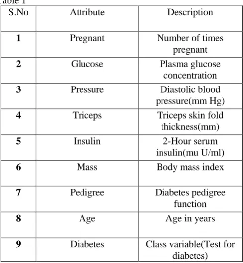
The dataset has been imported from[1] and it was collected by the US National Institute of Diabetes and Digestive and Kidney Diseases. It has a total of 768 instances with 9 attributes which includes a class label as well among the given attributes and all the attributes are numeric in nature. Among the total number of instances 268 are tested positive and 500 are tested negative for diabetes and this is

indicated by a class value of 1 and 0 in class label attribute. A brief description of attributes is given below:

Table 1

S.No Attribute Description

1 Pregnant Number of times

pregnant

2 Glucose Plasma glucose

concentration

3 Pressure Diastolic blood

pressure(mm Hg)

4 Triceps Triceps skin fold

thickness(mm)

5 Insulin 2-Hour serum

insulin(mu U/ml)

6 Mass Body mass index

7 Pedigree Diabetes pedigree

function

8 Age Age in years

9 Diabetes Class variable(Test for diabetes)

B. Supervised Classification Algorithms

Tree Algorithms

Naive Bayes

Naive Bayes finds the probabilty of specific outcome by counting the number of times numerious conditions are observed in an attempt to find and represent the relationship and pattern in the data set[5]. Bayes theorem can be useful for making predictions from such relationships.Bayesian classifiers are also known by the name naive Bayesian classifier.These classifiers possess high accuracy and speed in predicting the categorical classes when applied to large databases[5].This classifier has minimum error when compared to other classifiers and hence more effective[4].

Artificial Neural Network

Neural Network(NN)is most widely used but is very less interpretable[6][7]. This is basically mathematical model that mimics the human brain and has been used in sound,image and pattern recognition.Here input , hidden and output units are connected using edges containing weights[8]. We train a neural network by adjusting the weights that are initially randomly assigned so as to minimize the error[4][6].

Instance-based learning

Instance-based learning lies under the category of statistical methods. The Instance-based learning algorithms are also called as lazy-learning algorithms[9], because they perform the generalization or induction process at last when classification is performed. They require a smaller amount of time for computation in the training phase compared to eager-learners (such as neural, Bayes nets and decision trees) but require more computation time for classification process. Nearest Neighbour algorithms is one of the most simple instance-based learning algorithms. (kNN) K-Nearest Neighbour works on the principle that, objects which have similar properties will generally be in close nearness to other object within a dataset[10] . The tag of an unclassified object can be found by finding the class of its adjacent neighbours, if the objects are tagged with a classification label. The class is determined by kNN by identifying the particular mainly frequent class tag.

Support Vector Machines

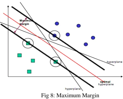
The latest supervised machine learning technique is Support Vector Machines (SVMs)[11].In SVMs the two data classes are separated by hyperplane. Maximizing the margin space between the separating hyper plane and the objects on each side of it .It has been confirmed to decrease an upper bound on the likely generalization error. A pair (w,b) exists if the training data is linearly separable, such that

An optimum separating hyperplane can be created by reduction of the squared norm of the separating hyperplane. It is easy to show that, when it is feasible to linearly divide two classes using a convex quadratic programming problem, then minimization can be set up as follows:

Once the optimum separating hyperplane is set up, in the case of linearly separable data, the points that are positioned on its margin are called as support vectors and the result is shown as a linear combination of just these points (see Figure 8). Further data points are overlooked.

Fig 8: Maximum Margin

The number of attributes that are encountered in the training dataset (the number of support vectors selected by the SVM learning algorithm is usually little). This is the reason that the complexity of SVM model is unaffected by the number of instances.

C. EVALUATION MEASURES

The explanation of some of performance evaluation measures is shown as under:

Accuracy (Correct Rate) = Number of cases correctly diagnosed/Total number of cases.

Error Rate=Number of cases incorrectly diagnosed/Total number of cases.

Sensitivity=Number of positive cases correctly diagnosed/Total number of positive cases.

Specificity=Number of negative cases correctly diagnosed/Total number of negative cases.

Confusion matrix:-Confusion matrix[12] is also used for evaluating the performance of the classification system it consists of information regarding the predicted classification and actual classification. The confusion matrix is shown below in table 6 which for a two class classifier.

True Positive (TP) – Correct Positive Prediction False Positive (FP) – Incorrect Positive Prediction True Negative (TN) – Correct Negative Prediction False Negative (FN) – Incorrect Negative Prediction These four categories are represented by the Confusion Matrix as below:

Table 2:Confusion matrix showing the four categories.

Actual Predicted

Negativ e

Positiv e

Negative TN FN

Positive FP TP

We would always like to have FP and FN as zero the less value of these two groups in confusion matrix the better is the classification of a classifier.

III. Experiments and Results

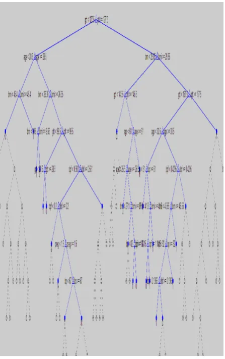
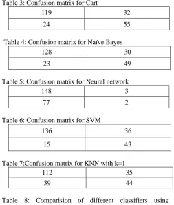
In this section we present the results of experiments using different machine learning classifiers by making use of MATLAB 2014 with the hardware confugration of Intel(R) Core(TM) i3 CPU M 370 @ 2.40 GHz 2.39 GHz processor with 2 GB RAM. Holdout validation has been used because dataset contains good number of instances , where 70% of instances have been used for training purpose and the rest 30% for testing purpose Each experiment has been repated five times and the mean of the measures has been mentioned in the tables so as to avoid the impact of extraneous varibles.Moreover for KNN and Neural network classifiers only change in parameters is shown twice in table 8 for each experiment so as to keep the size of the table limited. Among the tree algorithms the classification and regression tree (CART) has been used for classification of pima indian diabetes data set and the view of the tree formed is shown below in Fig1, confusion matrix is shown in table 3,ROC curve is depicted in fig 2 and the others measures are accuracy=0.7565,error rate=0.2435, Sensitivity=0.7881, Specificity=0.6962 and AUC =0.7421. The Naive Bayes technique has been used on the same data set its confusion matrix is shown in table 4,ROC curve in fig 3 and the other measures are accuracy=0.7696,error rate=0.2304, Sensitivity=0.8101, Specificity=0.6806and AUC =0.7453.The Neural network has been implemented on the data set and the training phase consists of 1000 epochs as this has been set as stopping criteria for traininng the neural network as is shown in fig4,confusion matrix for this is shown in table 5,ROC curve is shown in fig5 and the other measures are accuracy=0.6522,error rate=0.3478, Sensitivity=0.9801, Specificity=0.0253and AUC =0.5027.And we have also changed epoch parameter and observed the changes in performance of the classifier thus by observing the impact of tuning the parameter of this classifier.The Support vector machines( SVM ) has been implemented on pima indian diabetes data set and its confusion matrix is shown in table 6,ROC curve in fig 6 and its accuracy=0.7783,error rate=0.2217, Sensitivity=0.7907, Specificity=0.7414 and AUC =0.7660.The last technique that falls under the category of lazy learners called KNN technique has been used on the same benchmark data set and its confusion matrix is shown in table 6,its ROC curve in fig 7 and its accuracy=0.6783,error rate=0.3217,

Sensitivity=0.7619, Specificity=0.5301and AUC =0.6460 and similarly for this classifier parameters were changed /tuned over several runs and the change in performance observed and recorded as shown in table 8.In (Table 8) it may seem that (SVM) outperforms all other algorithms except for Naïve Bayes and Neural Networks in case of sensitivity measure. But in case of diabetic diagnosis this measure is of vital importance. This is basically the proportion of positive cases that are correctly labeled. And the other measure specificity is proportion of negative cases that are correctly labeled. If a case detected as diabetic which is actually non diabetic does not matter much as is the case if a patient is diabetic and diagnosed as non diabetic because diabetes is a chronic disease a patient may lose his life. This is the reason why this measure is of vital importance. And neural network perform the best with respect to this parameter. And further improvements are possible by tuning the parameters as analyzed experimentally.

Fig 2: ROC Curve for CART Classifier

Fig 3: ROC Curve for Naive Bayes Classifier

Fig 4: Neural network training with epoch 1000

Fig 5: ROC Curve for Neural network Classifier with epoch 1000

Fig 6: ROC Curve for SVM Classifier

Table 3: Confusion matrix for Cart

119 32

24 55

Table 4: Confusion matrix for Naïve Bayes

128 30

23 49

Table 5: Confusion matrix for Neural network

148 3

77 2

Table 6: Confusion matrix for SVM

136 36

15 43

Table 7:Confusion matrix for KNN with k=1

112 35

39 44

Table 8: Comparision of different classifiers using performance metrics

IV. CONCLUSION

This paper presents the classification of diabetic dataset without taking in to consideration the computational time

and the nature of classification algorithms. The main focus is on checking classification accuracy and other performance measures of automatic classifiers and the classifiers that require expert intervention for tuning up the parameters. Moreover there is the blend of automatic and non-automatic machine learning techniques used on this benchmark dataset that adds to the variance in accuracy and other performance measures across different algorithms used for diagnosis of diabetic disease. Finally we conclude that neural networks outperforms all the above given algorithms for diabetic diagnosis. Parameter tuning capability of a researcher may further improve the diagnosis of diabetes as is evident by changing certain parameters in the experiments. Parameter tuning and has a major importance in diagnosing diabetes.

V. REFERENCES

[1] www.archive.ics.uci.edu/ml/datasets.html [2] www.diabetes.org.uk/Guide-to-diabetes what-is-diabetes/what-is-Type—2 Diabetes.

[3] www.idf.org/worlddiabetesday/toolkit/gp/facts-figures [4] Han, Jiawei, Micheline Kamber, and Jian Pei. Data mining:

concepts and techniques, second Edition (The Morgan Kaufmann Series in Data management Systems). Morgan aufmann, San Franscisco, CA, USA,2 edition, January 2006. [5] Berger, C., Oracle Data Mining, Know More, Spend

Less-An Oracle White paper,(2004).

[6] Berry, Michael JA, and Gordon S.Linoff. Mastering data mining:the art and science of customer relationship management. Amazon, 2006.

[7] Hinton, G.E . and Sejnowski, T.J.Unsupervised learning: Foundations of neural Computation, MIT press, Cambridge, MA, MIT Press publishers, (1999), www.elsevier.com/locate/tcs

[8] Pyle, Dorian. Data preparation for data mining. Vol. 1. Morgan Kaufmann, 1999.

[9] Rumelhart, D. E., Hinton, G. E., Williams, R. J.(1986), Learning internal representations by error propagation. In: Rumelhart D E, McClelland J L et al. (eds.) Parallel Distributed Processing: Explorations in the Microstructure of Cognition. MIT Press, Cambridge, MA, Vol. 1, pp. 318-362. [10] Cover, T., Hart, P. (1967), Nearest neighbor pattern

classification. IEEE Transactions on Information Theory, 13(1): 21–7.

[11] Vapnik, V. (1995), The Nature of Statistical Learning Theory}. Springer Verlag.

[12] Jeff Schneider’s home page,http://www.cs.cmu.edu/~schneide/tut5/node42.html.