The effects of oar-shaft stiffness and length on rowing biomechanics

(1)

Western University Western University

Scholarship@Western

Electronic Thesis and Dissertation Repository

8-15-2014 12:00 AM

The effects of oar-shaft stiffness and length on rowing

biomechanics

Brock Laschowski

The University of Western Ontario

Supervisor Dr. Volker Nolte

The University of Western Ontario Graduate Program in Kinesiology

A thesis submitted in partial fulfillment of the requirements for the degree in Master of Science © Brock Laschowski 2014

Follow this and additional works at: https://ir.lib.uwo.ca/etd

(2)

THE EFFECTS OF OAR-SHAFT STIFFNESS AND LENGTH ON ROWING BIOMECHANICS

(Thesis format: Integrated Article)

by

Brock Laschowski

Graduate Program in Kinesiology

A thesis submitted in partial fulfillment of the requirements for the degree of

Masters of Science

The School of Graduate and Postdoctoral Studies The University of Western Ontario

London, Ontario, Canada

(3)

Abstract

This work investigates the effects of oar-shaft stiffness and length on rowing biomechanics. The mechanical properties of the oar-shafts were examined using an end-loaded cantilever system, and theoretical relations were proposed

between the mechanics of the oar-shafts and rowing performance. On-water experiments were subsequently conducted and rowing biomechanics measured via the PowerLine Rowing Instrumentation System. The PowerLine system measures force and oar angle on the oarlock, as well as proper boat

acceleration. The convergent validity and test-retest reliability of the PowerLine force measurements were determined prior to the on-water experiments. Thereafter, rowers were tested over a set distance using oar-shafts of different stiffness and length. There were slight differences in the biomechanics between rowing with the different oar configurations. However, the measured differences in the biomechanical parameters were on the same order of magnitude as the rower’s inter-stroke inconsistencies.

Keywords

(4)

Co

-

Authorship Statement

(5)

Acknowledgments

I want to thank:

- Dr. Volker Nolte, my MSc supervisor

- Dr. John de Bruyn and Cameron Hopkins from the Department of Physics and Astronomy

- Michael Adamovsky and Ryan Alexander from the Faculty of Engineering - Will George from the Canadian Sport Institute Ontario

- Dr. Daniel Bechard and Matt Waddell from the Western Rowing Program - Katherine Cornacchia, my fiancé

(6)

List of Tables

Table 1. The twelve oar configurations that were investigated. Each configuration is designated by a code that indicates the stiffness (M or ES), side (P or S), and total length of the oar. The total length of the oar varied by changing Lb. ... 11

Table 2. The flexural rigidity EI (Nm2) for each oar configuration at each position

yi along the oar-shaft. The uncertainties are SD. ... 18

Table 3. The deflection angles θ at the blade-end of the oar-shafts for each

configuration when loaded with 201.04 N. The uncertainties are SD. ... 20

Table 4. Analyzing normality of the PL force measurements as a function of the testing date using a Shapiro–Wilk test. ... 31

Table 5. Investigating normality of the PL force measurements as a function of the known static forces using a Shapiro–Wilk test. ... 33

Table 6. Testing the convergent validity of the PL force measurements using a Wilcoxon One-Sample Signed Rank Test. ... 34

Table 7. The slope, y-intercept and R2 for the PL force measurements as a function of the known static forces from a least-squares linear regression

analysis. ... 37

Table 8. The six oar configurations that were tested. Each configuration is

(10)

Table 11. Average wind velocity (m/s) measured along the testing course during trials 1-6 for each rower. ... 48

Table 12. The maximum force (N), % of the drive to maximum force, and impulse (Ns) measured on port and starboard oarlocks for each oar configuration for all four rowers. The results are given by the mean ± SD over 20 strokes. ... 54

(11)

List of Figures

Figure 1. Schematic of the rowing boat from an aerial view. The components of the boat are discussed in the text. ... 2

Figure 2. Schematic of the rowing oar. The properties of the oar are discussed in the text. ... 3

Figure 3. The locations of the seat and oars at the catch [grey] and finish [black] positions. The oar angles are 0° when the oars are perpendicular to the boat’s main direction of motion. ... 4

Figure 4. Photograph of a sweep oar-shaft during on-water rowing with visible deflection. ... 9

Figure 5. Schematic of the setup used to measure the oar-shaft’s deflection from its equilibrium position Ex at six positions yi along the shaft when a static

load W is applied at length Lb from Clamp 2. The support length Ls is the distance between Clamps 1 and 2. The deflection angle at the blade-end of the oar-shaft is denoted by θ. ... 10

Figure 6. Photograph of the experimental set-up used to measure oar-shaft deflection. The oar is secured to a laboratory bench with a custom-made support stand, and a weight plate is suspended from the oar-shaft using a tether. ... 12

(12)

Figure 10. Flexural rigidity EI as a function of position y for port and starboard versions of Oar M. The three data points in each group correspond to oar lengths of 2.66, 2.68, and 2.70 m, as shown by the sketched curves. ... 17

Figure 11. Deflection angles θ at the blade-end of the oar-shafts for MP2.70 and ESP2.70 as a function of load W. The linear fits are expressions to equation (3). ... 19

Figure 12. Orientating the PL swivel perpendicular to the base of the inner tube (shown in the left side of the photograph) using a spirit level. ... 28

Figure 13. Photograph of the experimental setup used to test the PL oarlocks. A bar is supported by two stands, and a PL oarlock is fixed to the bar. The PL swivel is pointed in the x-direction and the base of the inner tube is pointed in the

y-direction. The PL oarlock is connected to a data-logger, and a suspension rig is hanging from the oarlock. ... 29

Figure 14. The PL force measurements as a function of the known static forces for a single sculling oarlock. The linear fit is a regression line. ... 35

Figure 15. Schematic of the oar-shaft’s dynamic behavior during the drive. The equilibrium position Ex refers to the point where the magnitude of the oar-shaft’s deflection in the x-axis is zero. δ is deflection and δ-1 is inverse deflection, as described in the text. Deflection of the inboard is neglected in this model. ... 43

Figure 16. Free body diagram of the external forces that act on the rowing oar during the drive. Fh is the force applied by the rower to the handle, Fo is the

normal reaction force at the oarlock, M is the resultant moment of force, Fb is the

load on the blade, Lbʹ′ is the beam moment arm, and Lsʹ′ is the support moment arm. ... 44

(13)

Figure 18. Boat acceleration as a percentage of the drive between ES2.70 and M2.70 for rower 2. The fits to the data are smoothing splines. ... 51

Figure 21. Oarlock force as a function of angle between ES2.70 and M2.70 for rower 1 on port side. The fits are smoothing splines. ... 56

Figure 25. Oarlock force as a function of angle between M2.66 and M2.70 for rower 1 on port side. The fits are smoothing splines. ... 59

Figure 26. Oarlock force as a function of angle between M2.66 and M2.70 for rower 2 on port side. The fits are smoothing splines. ... 59

(14)

List of

Nomenclature

AOA Angle of attack (°)

M Medium oar-shaft

ES Extra-Soft oar-shaft

yi Position on the oar-shaft in the y-axis (m)

W Static load (N)

Lb Beam length (m)

Ls Support length (m)

θ Angle of deflection (°)

δ Deflection (m)

P Port

S Starboard

E Young's modulus (N/m2)

I Area moment of inertia (m4)

EI Flexural rigidity (N·m2)

PL PowerLine

Re Electrical resistance (Ω)

ρ Electrical resistivity (Ω·m)

Lg Length of strain gauge (m)

A Cross-sectional area (m2)

R2 _{Coefficient of determination}

Ho Null hypothesis

SD Standard deviation

Ex Equilibrium position of oar-shaft in x-axis

Fl Lift force (N)

Fd Drag force (N)

cl Lift coefficient

cd Drag coefficient

(15)

Aʹ′ Reference area (m2)

α Angular acceleration (rad/s2)

ρw Density of water (kg/m3)

Fdiff Difference in force (N)

ANOVA Analysis of variance

Lbʹ′ Beam moment arm (m)

Lsʹ′ Support moment arm (m)

Fh Handle force (N)

Fb Blade force (N)

Fo Oarlock force (N)

M Moment of force (N·m)

Im Mass moment of inertia (kg·m2)

Fmax Maximum force (N)

Fmax% Percentage of drive to Fmax (%)

r Pearson product-moment correlation coefficient

δ-1 Inverse deflection (m)

𝒙 Arithmetic mean

x, y, z Three-dimensional Cartesian coordinate system

(16)

Chapter 1

1 General Introduction

1.1 Rowing

The main objective in competitive rowing is for a rower to cover a 2000 m race distance, in a rowing boat, in the least amount of time. Rowing is divided into two classes: sweep and sculling. In sweep, the rower rows with one oar gripped with both hands. There are three types of sweep boats: the pair (i.e., two rowers), the four (i.e., four rowers) and the eight (i.e., eight rowers). In sculling, the rower rows with one oar in each hand simultaneously. There are three types of sculling boats: the single (i.e., one rower), the double (i.e., two rowers) and the quad (i.e., four rowers). The following work will pertain to single sculling unless otherwise specified.

1.1.1 Boat

(17)

Figure 1. Schematic of the rowing boat from an aerial view. The components of the boat are discussed in the text.

The shell is the supporting structure of the boat that interacts with the water. A wing rigger is mounted on top of the shell, and extends outward from the centerline of the boat in the port and starboard directions. Cylindrical pins at the ends of the wing rigger extend upward in the z-axis. “Oarlocks” slide onto the pins and feature U-shaped channels that are used to support the oars on the wing rigger. Throughout the rowing stroke, the oars rotate with the oarlocks around the pins in the z-axis.

1.1.2 Oar

Figure 2 illustrates the components of the rowing oar. The blade is the

cleaver-Bow Stern

Direction of Motion

Blade Oarlock

x y

Wing Rigger

Shell Port

Starboard

(18)

the collar to the tip of the handle. The total length of the oar is the sum of the outboard and inboard lengths.

Figure 2. Schematic of the rowing oar. The properties of the oar are discussed in the text.

1.1.3 Stroke

The rowing stroke is divided into two positions (i.e., catch and finish) and two phases (i.e., drive and recovery). The oar angles are defined by their rotation around the pins in the z-axis. The catch position is the point where the handles are closest to the stern; it has the highest magnitude of negative oar angle and is defined as the start of the rowing stroke (Figure 3). Following the catch position, the blades enter the water and the rower pulls on the handles. As the handles move towards the bow, the oar angles decrease in negative magnitude. The oar angles are considered to be 0° when the oars are perpendicular to the boat’s main direction of motion [1-2], as illustrated in Figure 3. Passing the

perpendicular position, the oar angles increase in positive magnitude as the handles move towards the bow. The finish position is the point in the stroke where the handles are closest to the bow, which has the highest magnitude of positive oar angle. Typical catch and finish angles for an elite heavyweight female sculling rower, averaged over 20 strokes at a rate of 20 strokes/min, is purportedly 63.2 ± 1.2° and 44.0 ± 0.9°, respectively (Canadian Sport Institute Ontario, 2014, personal communication). The blades are removed from the water slightly before the finish. The drive phase is the motion from the catch to the finish position, and the recovery phase is the motion from the finish position back to the catch.

Outboard Length Inboard Length

Handle _Collar

Sleeve

(19)

Figure 3. The locations of the seat and oars at the catch [grey] and finish [black] positions. The oar angles are 0° when the oars are perpendicular to the boat’s

main direction of motion.

1.2 Current Research

Rowing oar-shafts are engineered in a variety of circumferences, lengths, materials and structural designs. However, the effects of these properties on rowing performance are not well known. This is particularly true for oar-shaft stiffness, as many previous studies have assumed that the shaft is perfectly rigid [3-13]. In addition, the effect of oar length on rowing performance is widely

discussed. For many years, rower’s opted for longer oars because increasing oar length was associated with greater force on the blade [14]. Recently, Nolte [15]

x y

Catch Position

Finish Position

0°

(-) (+)

(20)

1.3 References

1. Dal Monte A and Komor A. Rowing and sculling mechanics. In: Vaughan CL (eds) Biomechanics of Sport. USA: CRC Press, 1989, pp.53-119.

2. Nolte V. Die Effektivität des Ruderschlages. [The efficiency of the rowing stroke.] Germany: Bartels and Wernitz, 1984.

3. Affeld K, Schichl K and Ziemann A. Assessment of rowing efficiency.

International Journal of Sports Medicine 1993; 14: 39-41.

4. Alexander FH. The theory of rowing. Proceedings of the University of Durham Philosophical Society 1925, pp.160-179.

5. Baudouin A and Hawkins D. A biomechanical review of factors affecting rowing performance. British Journal of Sports Medicine 2002; 36: 396-402.

6. Brearley MN and De Mestre NJ. Modeling the rowing stroke and increasing its efficiency. In: The third Conference on Mathematics and Computers in Sport, Bond University, Queensland, Australia, 30 Sept–2 Oct 1996, pp.35–46.

7. Cabrera D, Ruina A and Kleshnev V. A Simple 1+ Dimensional Model of Rowing Mimics Observed Forces and Motions. Human Movement Science 2006; 25: 192-220.

8. Findlay M and Turnock SR. Mechanics of a rowing stroke: Surge speed variations of a single scull. Proceedings of the Institution of Mechanical

Engineers, Part P: Journal of Sports Engineering and Technology 2010; 224: 89-100.

(21)

10. Macrossan MN and Macrossan NW. Energy efficiency of the rowing oar from catch to square-off. Report, University of Queensland, Australia, May 2008.

11. Sanderson B and Martindale W. Towards optimizing rowing technique.

Medicine and Science in Sports and Exercise 1986; 18: 454-468.

12. Serveto S, Barre S, Kobus JM and Mariot JP. A three-dimensional model of the boat–oars–rower system using ADAMS and LifeMOD commercial software.

Proceedings of the Institution of Mechanical Engineers, Part P: Journal of Sports Engineering and Technology 2010; 224: 75-88.

13. Zatsiorsky VM and Yakunin N. Mechanics and biomechanics of rowing: A review. International Journal of Sport Biomechanics 1991; 7: 229-281.

14. Adam K, Lenk H, Nowacki P, Rulffs M and Schröder W. Rudertraining. [Rowing training.] Germany: Limpert, 1977.

15. Nolte V. Shorter Oars Are More Effective. Journal of Applied Biomechanics

2009; 25: 1-8.

16. Hofmijster M, De Koning J and Van Soest AJ. Estimation of the energy loss at the blades in rowing: Common assumptions revisited. Journal of Sports Science 2010; 28: 1093-1102.

(22)

Chapter 2

2 The Mechanical Properties of

Oar

-

Shafts

2.1 Introduction

Rowing oar-shafts transfer force applied to the handles by the rower to the blades, which act on the water to propel the boat. The oar-shaft’s efficiency [1] in transferring force is affected by its mechanical design and material composition. Until the 1980s, oar-shafts were predominantly made out of Sitka spruce from the northern United States and Canada because their shorter growing seasons produced a finer grain [2, 3]. The wood was cut into strips, laminated, shelved for weeks, and finished by hand cutting and polishing [3-5]. Ash was occasionally glued onto the oar-shafts for added durability [4]. The Sitka spruce oar-shafts tapered from the sleeves towards the blades [5], and had masses of 4 to 4.3 kg [3].

Most present-day oar-shafts are engineered from composite materials, like carbon fiber reinforced polymers that are cured at high temperatures [2-4, 6]. These composite shafts are stiffer, and up to 60 % lighter, than wood oar-shafts [4-6]. Oar manufacturers typically classify a shaft’s stiffness based on its deflection at the junction between the shaft and the blade, when a static load of 98.1 N is applied to the junction area [7-9]. Its stiffness can be affected by the amount and distribution of high-modulus carbon fiber. For instance, Concept2 designs and markets “Extra-Soft” shafts, which contain approximately 20 % high modulus carbon fiber, and “Medium” stiffness oar-shafts with about 40 %;

(23)

The mechanical properties of rowing oar-shafts are not well known. Many previous studies have assumed that the oar-shaft is perfectly rigid [10-20]. This assumption is simple but unrealistic, since oar-shaft deflections can be seen with the naked eye during on-water rowing (Figure 4). Sliasas and Tullis [21]

(24)

Figure 4. Photograph of a sweep oar-shaft during on-water rowing with visible deflection.

(25)

2.2 Methods

Two sets of sculling oars with “skinny” shafts (Concept2 Inc., Vermont, United States) of different stiffness were investigated. Medium oar-shafts, which are designed to deflect 0.045 ± 0.002 m at the junction between the shaft and the blade when loaded with 98.1 N, are referred to as “M” oars; oar-shafts denoted as “ES” are Extra-Soft and designed to deflect 0.065 ± 0.002 m [8]. The

circumferences of OarM and OarES both taper from 0.111 m at the sleeves to 0.108 m at the blades. OarM and OarES have masses of 1.4 and 1.3 kg, respectively.

Figure 5. Schematic of the setup used to measure the oar-shaft’s deflection from

Static Load (W) Clamp 1 Clamp 2

Support Length

(L_s) y₁ y₂ y₃ y₄ y₅ y₆

Beam Length (L_b) Total Length

y

x

θ Deflection

Angle

(26)

between Clamps 1 and 2 (i.e., the support length Ls) was fixed at 0.715 m. The beam length Lb is the distance between the load and Clamp 2, and ranged between 1.279 and 1.319 m. The total length of the oars, which were set to 2.66, 2.68 and 2.70 m, varied by changing Lb. All length measurements were taken with a ± 9 × 10-5_{m tolerance (Lufkin, Texas, USA). The oars have a built-in}

length adjustment system, whereby the oar can adjust up to 0.05 m in total length [8]. Six positions were marked along the oar-shafts at y1-6measured from Clamp 2 (i.e., where y is zero). A digital height gage (Mitutoyo Inc., Quebec, Canada), with a ± 5 × 10-5_{m tolerance, was used to measure the linear deflection}_δ_{in the}

x-axis at positions y1-6 relative to the oar-shafts equilibrium position Ex. Port (P) and starboard (S) versions of OarM and Oar ES were tested with three different lengths, for a total of twelve configurations (Table 1).

Table 1. The twelve oar configurations that were investigated. Each configuration is designated by a code that indicates the stiffness (M or ES), side (P or S), and

total length of the oar. The total length of the oar varied by changing Lb.

Code Stiffness Side Total Length (m) Lb (m)

MP2.66 Medium Port 2.66 1.279

MS2.66 Medium Starboard 2.66 1.279

ESP2.66 Extra-Soft Port 2.66 1.279

ESS2.66 Extra-Soft Starboard 2.66 1.279

ESS2.68 Extra-Soft Starboard 2.68 1.299

(27)

Static loads W of 12.75, 21.57, 41.19, 111.8, 152, and 201.04 N were individually applied to the oars at distances Lb from Clamp 2 by suspending weight plates from the shafts using a tether. The weights of the plates and tether were measured using a digital bench scale (Rice Lake Weighing Systems, Wisconsin, United States) with an engineering tolerance of ± 0.98 N. The range of W was chosen to parallel the range of forces previously estimated on the blade during on-water rowing [22]. Four measurement trials were conducted for each value of Wand y, and the results are arithmetic means with the

uncertainties given by standard deviations SD. Error bars are not included in the figures because they were smaller than the symbols. This demonstrates that any measurement errors are substantially smaller than the measured deflections. All figures were generated in MATLAB 2013a (The MathWorks Inc., Massachusetts, USA).

(28)

between the two oars increased with distance towards the blades. This trend was seen in all the configurations over the range of W studied. Deflection data were fit to the expression for the deflection of an end-loaded cantilever beam with a homogenous cross-section [25] given by

𝛅_!_! =𝑾_!!!_!"! (3𝐿_!−𝑦_!) (1)

where E is the Young’s modulus, I is the area moment of inertia, and the

combination EI is the flexural rigidity. The weight of the beam is neglected in this model. Since the values of W and Lb are known, EI was the only fitting

(29)

Figure 7. Deflection δ as a function of position y for MP2.70 and ESP2.70 when loaded with 111.8 N. The curves are fits to equation (1).

0 0.2 0.4 0.6 0.8 1 1.2 1.4

0 0.01 0.02 0.03 0.04 0.05 0.06

Position y (m)

Deflection

(m)

(30)

Figure 8. Deflectionδ as a function of load W for MP2.66 at three positions yi along the oar-shaft. The lines are fits to the data discussed in the

text.

Figure 8 shows δ as a function of W for MP2.66 at three positions y. At each yi, δ was accurately proportional to W, as expected from Hooke’s Law; this trend was seen in all the configurations. The slope m of the data for a given yi is the compliance of the oar-shaft at that position, and is related to the flexural rigidity EI via

𝐸𝐼_!_! = _!!!!!

!_! (3𝐿!−𝑦!) (2)

Typical results for EI as a function of y are illustrated for two oar

configurations in Figure 9. Both oars are most compliant near the sleeves and become progressively stiffer towards the blades. Similar results were seen in all

0 20 40 60 80 100 120 140 160 180 200

0 0.01 0.02 0.03 0.04 0.05 0.06 0.07

Load W (N)

Deflection

(m)

(31)

the configurations whereby the blade-end of the oar-shafts are stiffer, by up to 64.4 % for Oar M and 78.9 % for Oar ES, than compared to near the sleeves. In Figure 9, EI is approximately 33.9 % larger for Oar M than Oar ES.

Figure 9. Flexural rigidity EI as a function of position y for MP2.70 and ESP2.70.

Figure 10 shows EI as a function of y for port and starboard versions of Oar M at three different lengths. For a given yi, increasing the oar length from

0.2 0.4 0.6 0.8 1 1.2 1.4

800 1000 1200 1400 1600 1800 2000 2200

Position y (m)

Flexural Rigidity

EI

(Nm

2 )

(32)

Figure 10. Flexural rigidity EI as a function of position y for port and starboard versions of Oar M. The three data points in each group correspond to oar lengths

of 2.66, 2.68, and 2.70 m, as shown by the sketched curves.

0.2 0.4 0.6 0.8 1 1.2 1.4

1200 1300 1400 1500 1600 1700 1800 1900 2000 2100 2200

Position y (m)

Flexural Rigidity

EI

(N m

2 )

MP MS

2.70

2.68

(33)

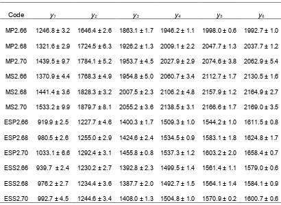
Table 2. The flexural rigidity EI (Nm2) for each oar configuration at each position

yi along the oar-shaft. The uncertainties are SD.

Code y1 y2 y3 y4 y5 y6

MP2.66 1246.8 ± 3.2 1646.4 ± 2.6 1863.1 ± 1.7 1946.2 ± 1.1 1998.0 ± 0.6 1992.7 ± 1.0

MP2.68 1321.6 ± 2.9 1724.5 ± 6.3 1926.2 ± 1.3 2009.1 ± 2.2 2047.7 ± 1.3 2037.7 ± 1.2

MP2.70 1439.5 ± 9.7 1784.1 ± 5.2 1953.7 ± 4.5 2027.9 ± 2.9 2074.6 ± 3.8 2062.9 ± 5.4

MS2.66 1370.9 ± 4.4 1768.3 ± 4.9 1954.8 ± 5.0 2060.7 ± 3.4 2112.7 ± 1.7 2130.5 ± 1.6

MS2.68 1441.4 ± 3.6 1828.3 ± 3.2 2007.5 ± 2.3 2106.2 ± 4.8 2157.9 ± 1.2 2164.9 ± 2.7

MS2.70 1533.2 ± 9.9 1879.7 ± 8.1 2055.2 ± 3.6 2138.5 ± 3.1 2166.6 ± 1.7 2169.0 ± 3.5

ESP2.66 919.9 ± 2.5 1227.7 ± 4.6 1400.3 ± 1.7 1509.3 ± 1.0 1544.2 ± 1.0 1611.5 ± 0.8

ESP2.68 980.5 ± 2.6 1255.0 ± 2.9 1424.6 ± 2.4 1534.5 ± 0.9 1583.1 ± 1.8 1624.8 ± 1.7

ESP2.70 1033.1 ± 6.6 1292.4 ± 3.1 1455.8 ± 0.8 1537.3 ± 1.2 1603.2 ± 2.0 1658.4 ± 0.7

ESS2.66 939.7 ± 2.4 1230.2 ± 2.7 1392.8 ± 2.3 1499.5 ± 1.4 1561.4 ± 1.1 1579.0 ± 0.6

ESS2.68 976.2 ± 2.7 1234.4 ± 3.6 1387.7 ± 2.0 1492.7 ± 1.5 1564.1 ± 1.4 1584.1 ± 0.9

ESS2.70 992.7 ± 4.5 1244.6 ± 3.4 1408.0 ± 1.3 1504.8 ± 1.0 1570.9 ± 0.2 1600.7 ± 0.6

The deflection angle θ was calculated from the tangent between the deflections at the two positions y5 and y6 at the blade-end of the oar-shafts, as illustrated in Figure 5. Figure 11 shows θ as a function of W for MP2.70 and ESP2.70. As expected, θ increased proportionally with W. The relative

(34)

Figure 11. Deflection angles θ at the blade-end of the oar-shafts for MP2.70 and ESP2.70 as a function of load W. The linear fits are expressions to equation (3).

Increasing oar length from 2.66 to 2.70 m increased θ by up to 0.20 ± 0.07° when loaded with 201.04 N. Similarly, there was a maximum difference in θ

of 0.22 ± 0.07° between port and starboard oars of the same stiffness and length. Table 3 shows the calculated values of θ for all twelve configurations.

0 20 40 60 80 100 120 140 160 180 200

0 1 2 3 4 5 6 7

Load W (N)

Deflection Angle

(

°

)

(35)

Table 3. The deflection angles θ at the blade-end of the oar-shafts for each configuration when loaded with 201.04 N. The uncertainties are SD.

Code Deflection Angle (°)

MP2.66 4.73 ± 0.002

MP2.68 4.77 ± 0.003

MP2.70 4.86 ± 0.013

MS2.66 4.42 ± 0.003

MS2.68 4.49 ± 0.006

MS2.70 4.62 ± 0.007

ESP2.66 5.85 ± 0.003

ESP2.68 5.98 ± 0.006

ESP2.70 6.04 ± 0.002

ESS2.66 5.97 ± 0.002

ESS2.68 6.13 ± 0.003

ESS2.70 6.26 ± 0.003

2.4 Discussion

The aim of this chapter was to investigate the mechanical properties of oar-shafts with different stiffness and length. Oars were clamped at the handles and

(36)

approximately 0.065 and 0.045 m when a static load of 98.1 N is applied at a distance of 1.50 m from the support [8]. To compare with the manufacturers specifications, the fits to deflection as a function of load at a beam length of 1.319 m were used to estimate the deflection at 98.1 N. The calculated

deflections for the Extra-Soft and Medium oar-shafts were approximately 30 and 22 % lower than the specified deflections. Since the oar-shafts are most

compliant near the sleeves and Concept2 uses a 12 % longer distance between the support and load, this could explain why Concept2 measures larger

deflections.

There were slight differences in the deflections between starboard and port oars of the same stiffness and length. This is likely not intentional, but rather a result of variations in the manufacturing process. It is expected that similar variations would be seen between, for example, several port oars. Asymmetric transfer of force from the handles to the port and starboard blades could produce a moment of force about the z-axis [10]. This would lead to what is known as yaw rotation. Yaw rotation has a negative effect on boat velocity, since altering the boat’s main direction of motion increases form drag on the underside of the shell [26-29]. However, differences in force between port and starboard oars are assumed to be predominately caused by the rower’s asymmetric application of force to the handles as oppose to any mechanical differences between the port and starboard oars, like the ones measured in this work.

The deflection angle at the blade-end of the oar-shaft was affected by both the oar-shaft’s stiffness and length. However, the effect of stiffness on the

(37)

sculling rower, averaged over 20 strokes at a rate of 20 strokes/min, is reported to be 109.1 ± 1.8° (Canadian Sport Institute Ontario, 2014, personal

communication). The change in deflection angle due to changing oar-shaft stiffness was thus smaller than the inter-stroke inconsistencies in the oar angles (i.e., the uncertainties) for an elite sculling rower.

The results show that the flexural rigidity of Concept2 oars is not constant along the shafts. For instance, differences of up to 775.30 Nm2 were calculated between the sleeve and the blade for MP2.66. The oar-shafts are most compliant near the sleeves and become progressively stiffer towards the blades. These findings can enhance the accuracy of numerical models that rely on the properties of the oar-shafts for input parameters because they provide more information than compared to previous research [21], which assumed a constant flexural rigidity of 8668 Nm2 along the Concept2 oar-shaft. In addition, since the location of the point of force application on the blade seemingly varies with respect to drive time [30], investigating the oar-shaft’s torsional rigidity presents an interesting topic future research.

(38)

3. Ashby MF. Materials selection in mechanical design. 3rd ed. UK: Elsevier Butterworth-Heinemann, 2005.

4. Boyne DJ. Essential Sculling: An Introduction to Basic Strokes, Equipment, Boat Handling, Technique, and Power. Canada: Globe Pequot Press, 2000.

5. Ritchie AC. Effect of Oar Design on the Efficiency of the Rowing Stroke. In: Subic A, Fuss FK and Ujihashi S (eds) The Impact of Technology on Sport II. UK: Taylor & Francis Group, 2007, pp.509-512.

6. Maybery K. Rowing: The essential guide to equipment and technique. UK: New Holland Publishers, 2002.

7. Macrossan MN. The direction of the water force on a rowing blade and its effect on efficiency. Report, University of Queensland, Australia, March 2008.

8. Concept2. Oar-Shafts Stiffness Options, http://www.concept2.com/oars/oar-options/shafts/stiffness (accessed 9 April 2014).

9. Brača-sport Rowing. Oar-Shaft Stiffness, http://rowing.braca-sport.com/oars/shafts/shaft-stiffness.html (accessed 9 April 2014).

10. Baudouin A and Hawkins D. A biomechanical review of factors affecting rowing performance. British Journal of Sports Medicine 2002; 36: 396-402.

11. Brearley MN and De Mestre NJ. Modeling the rowing stroke and increasing its efficiency. In: The third Conference on Mathematics and Computers in Sport, Bond University, Queensland, Australia, 30 Sept–2 Oct 1996, pp.35–46.

(39)

13. Hofmijster MJ, Landman EH, Smith RM and Van Soest AJ. Effect of stroke rate on the distribution of net mechanical power in rowing. Journal of Sports Sciences 2007; 25: 403-411.

14. Sanderson B and Martindale W. Towards optimizing rowing technique.

Medicine and Science in Sports and Exercise 1986; 18: 454-468.

15. Zatsiorsky VM and Yakunin N. Mechanics and biomechanics of rowing: A review. International Journal of Sport Biomechanics 1991; 7: 229-281.

16. Findlay M and Turnock SR. Mechanics of a rowing stroke: Surge speed variations of a single scull. Proceedings of the Institution of Mechanical

Engineers, Part P: Journal of Sports Engineering and Technology 2010; 224: 89-100.

17. Affeld K, Schichl K and Ziemann A. Assessment of rowing efficiency.

International Journal of Sports Medicine 1993; 14: 39-41.

18. Serveto S, Barre S, Kobus JM and Mariot JP. A three-dimensional model of the boat–oars–rower system using ADAMS and LifeMOD commercial software.

Proceedings of the Institution of Mechanical Engineers, Part P: Journal of Sports Engineering and Technology 2010; 224: 75-88.

19. Macrossan MN and Macrossan NW. Energy efficiency of the rowing oar from catch to square-off. Report, University of Queensland, Australia, May 2008.

(40)

22. Hofmijster M, De Koning J and Van Soest AJ. Estimation of the energy loss at the blades in rowing: Common assumptions revisited. Journal of Sports Science 2010; 28: 1093-1102.

23. Coppel A, Gardner T, Caplan N and Hargreaves D. Simulating the fluid dynamic behaviour of oar blades in competition rowing. Proceedings of the Institution of Mechanical Engineers Part P – Journal of Sports Engineering and Technology 2010; 224: 25-35.

24. Nolte V. Shorter Oars Are More Effective. Journal of Applied Biomechanics

2009; 25: 1-8.

25. Gere JM. Mechanics of Materials. 5th ed. USA: Brooks/Cole Publishing Company, 2002.

26. Schneider E and Hauser M. Biomechanical analysis of performance in rowing. In: Morecki A, Fidelus K, Kedzior K and Wit A (eds) Biomechanics VII-B. USA: University Park Press, 1981, pp.430–435.

27. Smith RM and Spinks WL. Discriminant analysis of biomechanical differences between novice, good and elite rowers. Journal of Sports Science 1995; 13: 377– 385.

28. Loschner C, Smith R and Galloway M. Boat orientation and skill level in sculling boats. In: XVIII International Symposium on Biomechanics in Sports, The Chinese University of Hong Kong, Hong Kong, June 25 2000.

29. Wing AM and Woodburn C. The coordination and consistency of rowers in a racing eight. Journal of Sports Science 1995; 13: 187-197.

30. Kinoshita T, Miyashita M, Kobayashi H and Hino T. Rowing Velocity

(41)

Chapter 3

3 Validity and

Reliability of the PowerLine Rowing

Instrumentation System

3.1 Introduction

The PowerLine (PL) Rowing Instrumentation System features replacement oarlocks that include strain gauge load cells, which quantify force at 50 Hz. The load cell consists of three concentric tubes connected in series [1]. The inner tube fits onto the pin of a wing rigger and has a locking mechanism that prevents its rotation around the pin [1]. A swivel fits onto the outer tube of the load cell and can rotate freely; four strain gauges are bound to the middle tube [1]. Individual strain gauges work on the concept of electrical resistance Re,

𝑅_! =𝜌!!

! (4)

where ρ represents the material’s electrical resistivity, Lg is the length of the gauge and A is its cross-sectional area [2]. When force is applied to an instrumented oarlock, its material deforms, the gauge responds to the elastic deformation of the oarlock’s material (i.e., by changing Lg and A) and the

(42)

main motion. In other words, the PL oarlocks are engineered to be insensitive to the forces applied in the orthogonal and vertical directions. The PL force

measurements were originally sensitive to the location of the point of force application [1]. Accordingly, the PL oarlocks were reengineered to use voltage outputs from two Wheatstone half-bridges to estimate the location of an applied force on the face of the PL swivel and automatically calibrate the force

measurements [1]. The PL force measurements have an engineering tolerance of ± 2 % of the force measurement [3].

Many national rowing programs use the PL system including Great Britain, South Africa, Brazil, New Zealand, France, Denmark, Netherlands, United States and Canada [3]. Despite its global popularity, only one independent study has investigated the validity of the PL force measurements [4]. Dynamic forces of up to 554.8 ± 20.4 N were manually applied to a loading bar that was suspended from the PL oarlocks with a load cell linked in series. The results of a linear regression analysis indicated excellent agreement between the PL and load cell measurements. The authors concluded that “the validity of the PL measurements were acceptable over the range tested in the laboratory” [4]. However, the

consistency of the PL force measurements over time has not been established, and previous research [4] has only tested the accuracy of PL scull oarlocks. Therefore, the following work investigates the convergent validity and test-retest reliability of the force measurements from sweep and scull PL oarlocks.

3.2 Methods

(43)

in a fixed direction (i.e., in the y-axis). The PL angle measurements have a ± 0.5° tolerance [3].

The inner tubes of the PL oarlocks were secured to a cylindrical bar that was supported by two squat stands; the bar represents the pin on a wing rigger. The bases of the inner tubes were orientated perpendicular to the PL swivels using a spirit level (Figure 12). The PL swivels were pointed in the x-direction and the bases of the inner tubes were pointed in the y-direction. Through this

(44)

Static forces of 0, 32.4, 255.1 and 431.6 N were individually applied to the PL oarlocks using a custom-made suspension rig that was loaded with weight plates. The suspension rig consisted of a box, wire cable and a loading bar connected in series (Figure 13). The weights of the plates and the suspension rig were measured using a digital bench scale (Rice Lake Weighing Systems,

Wisconsin, United States) with a ± 0.98 N tolerance. 0 N is the theoretical force on the oarlock when it points in the x-direction, 32.4 N is the weight of the suspension rig, and 255.1 and 431.6 N are the weights of the plates, which includes the weight of the suspension rig.

Figure 13. Photograph of the experimental setup used to test the PL oarlocks. A bar is supported by two stands, and a PL oarlock is fixed to the bar. The PL swivel is pointed in the x-direction and the base of the inner tube is pointed in the

(45)

The PL force measurements slightly fluctuate while the oarlocks are statically loaded – this was described as random error. Random error is

inherently unpredictable fluctuations in a measuring instrument [5], and can be reduced through calculating the arithmetic mean of multiple measurements [6]. The PL oarlocks were statically loaded for five seconds and the mean force measurement over that period was calculated and used in the analysis. Note that for a typical rowing drive, the duration of force application from the oar to the oarlock is approximately one second [7]. Data were collected over fifteen days and statistically analyzed using SPSSStatistics Version 21 (IBMCorp., Ontario, Canada). The statistical significance was set to .05, and the results are

presented with 95 % confidence.

3.3 Results

3.3.1 Test-Retest Reliability

Test-retest reliability is the consistency of an instrument to reproduce similar measurements over time [8]. The distributions of the PL force measurements were examined for normality and homogeneity of variance. Normality refers to a theoretical frequency distribution that is “bell-shaped” and symmetric about the mean [9]. A Shapiro–Wilk test [10] was used to test for normality in the

(46)

Table 4. Analyzing normality of the PL force measurements as a function of the testing date using a Shapiro–Wilk test.

Testing Date Sweep p-values Scull p-values

1 .000 .000

2 .269* .020

3 .018 .000

4 .008 .000

5 .001 .000

6 .357* .002

7 .045 .005

8 .000 .002

9 .002 .037

10 .000 .004

11 .005 .707*

12 .008 .028

13 .054* .000

14 .020 .046

15 .007 .030

Note: If the p-value is < .05, the results reject the Ho. An asterisk * indicates a normal distribution (p > .05).

Since the results were statistically significant, a non-parametric Levene’s F-test [11] was used to test for homogeneity of variance in the PL force

measurements over the fifteen days of testing. Data is homoscedastic if all

variables in a sample have similar variance [12]. In contrast, heteroscedasticity is when the variables in a sample have different variance [12]. The Ho is that there is homogeneity of variance. The p-values for sweep and scull oarlocks were .203 and .142, respectively. Since the p-values were > .05, the results fail to reject the

(47)

measurements as a function of the testing date. Although a parametric analysis of variance (ANOVA) can be robust to violations of normality [13], a

non-parametric model was selected to provide a more conservative analysis of the test-retest reliability of the PL force measurements. The reduced statistical power associated with non-parametric models was considered.

A Kruskal–Wallis One-Way ANOVA was used to determine the test-retest reliability of the PL force measurements over the fifteen days of testing; the analysis does not assume a normal distribution. The differences Fdiff between the

PL force measurements and the known static forces were calculated. The independent variable was the testing date and the dependant variable was the Fdiff. The Ho is that there is no difference in the Fdiff over the fifteen days of

testing. The p-values were .335 for scull and .451 for sweep oarlocks. Since the

p-values were > .05, the results fail to reject the Ho. This suggests that the PL force measurements were consistent over the fifteen days of testing. The maximum differences in the PL force measurements over the fifteen days of testing when loaded with 431.6 N, for instance, were 18.8 ± 11.9 N for sweep and 16.8 ± 6.2 N for scull oarlocks; the uncertainties are SD.

3.3.2 Convergent Validity

(48)

static forces. Since the majority of p-values were < .05 (Table 5), the results reject the Ho. This indicates that the PL force measurements are not normally distributed as a function of the known static forces. A non-parametric Levene’s F-test [11] was used to F-test for homogeneity of variance in the PL force

measurements as a function of the known static forces. The Ho is that there is homogeneity of variance in the distributions. The p-values for sweep and scull oarlocks were both .100. Since the p-values were > .05, the results fail to reject the Ho. This indicates homogeneity of variance in the PL force measurements over the range of forces that were tested.

Table 5. Investigating normality of the PL force measurements as a function of the known static forces using a Shapiro–Wilk test.

Known Force (N)

Sweep Force (N)

Sweep p-value Scull Force (N)

Scull p-value

0.0 0.1 ± 0.1 .000 0.1 ± 0.1 .000

32.4 31.5 ± 1.8 .000 31.7 ± 1.6 .100*

255.1 250.7 ± 3.6 .016 249.9 ± 4.1 .000

431.6 425.8 ± 5.5 .000 425.3 ± 5.1 .043

Note: If the p-value is < .05, the results reject the Ho. An asterisk * indicates a normal distribution (p > .05). The PL force measurements for all sweep and scull oarlocks, combined over the fifteen days of testing, are presented as the mean ±

SD for each load.

(49)

are shown in Table 6. Although the median PL force measurements were 98.1 % ± 0.8 percentage points (pp) of the values of the known static forces, the results rejected the Ho since the p-values were < .05. This is considered Type 1 error since the results rejected the Ho when, in reality, it was true. From this point forward, the convergent validity of the PL force measurements will be discussed numerically. Excluding the baseline measurements at 0 N, the median PL force measurements were slightly less than the values of the known static forces (i.e., 2.0 % ± 0.8 pp). The maximum differences between the PL force measurements and the known static forces were 15 ± 4 N for scull and 14 ± 7 N for sweep oarlocks.

Table 6. Testing the convergent validity of the PL force measurements using a Wilcoxon One-Sample Signed Rank Test.

Known Force (N) Median Sweep Force (N)

Sweep p-value Median Scull Force (N)

Scull p-value

0.0 0.1 .000 0.1 .000

32.4 31.3 .000 31.8 .000

255.1 250.2 .000 250.2 .000

431.6 425.6 .000 426.2 .000

Note: If the p-value is < .05, the results reject the Ho.

(50)

3.3.3 Calibration Factors

Calibration factors for each PL oarlock were established to correct for the slight discrepancies in the force measurements. Figure 14 shows an example of the PL force measurements as a function of the known static forces; the other PL

oarlocks showed a similar trend. There are no visual signs of heteroscedasticity, which is in agreement with the aforementioned results from the non-parametric Levene’s F-tests. A linear model was fit to the data using a least squares linear regression analysis generated in MATLAB 2013a (The MathWorks Inc.,

Massachusetts, USA). Though not shown here, the residuals were scattered randomly about the zero point.

Figure 14. The PL force measurements as a function of the known static forces for a single sculling oarlock. The linear fit is a regression line.

0 50 100 150 200 250 300 350 400 450 0

50 100 150 200 250 300 350 400 450

Known Force (N)

(51)

Table 7 shows the slope, coefficient of determination (R2) and y-intercept for the PL force measurements as a function of the known static forces. The R2 quantifies how well the linear regression fits the data [14]. The linear regressions accurately fit the data with R2_≥_{.999. In a calibration experiment, the linear}

(52)

Table 7. The slope, y-intercept and R2 for the PL force measurements as a function of the known static forces from a least-squares linear regression

analysis.

Type Oarlock ID Slope y-intercept y-intercept p-value

R2

Sweep 2664 .989 ± .003 -.18 ± .88 .837 .999

2442 .982 ± .002 -.52 ± .47 .273 1

2441 .985 ± .001 -.32 ± .38 .396 1

2435 .985 ± .003 -1.08 ± .76 .161 .999

2443 .983 ± .003 .39 ± .84 .644 .999

3214 .991 ± .002 -.08 ± .53 .880 1

3215 .991 ± .002 -.07 ± .41 .869 1

2665 .993 ± .002 -.38 ± .40 .338 1

2299 .978 ± .002 -.68 .47 .157 1

Scull 2305 .989 ± .001 .24 ± .36 .511 1

2444 .990 ± .002 -.38 ± .66 .570 1

2445 .987 ± .003 -.16 ± .70 .818 .999

2307 .982 ± .002 .18 ± .55 .752 .999

2447 .976 ± .003 -.75 ± .78 .343 .999

3646 .980 ± .002 .03 ± .60 .960 1

2446 .984 ± .002 -.87 ± .44 .055 1

2306 .989 ± .002 -.53 ± .53 .329 1

Note: The slope and y-intercepts for each PL oarlock are expressed as the coefficient ± SD. If the p-value is > .05, the results fail to reject the Ho.

3.4 Discussion

(53)

based technology, outside of human error, have been largely attributed to changes in temperature, pressure and humidity [15]. Considering that the PL oarlocks were stored and tested in a laboratory with a regulated room

temperature, it is somewhat expected that the PL force measurements were consistent over the fifteen days of testing. Since rowers compete on-water in a wide variety of weather conditions, investigating the test-retest reliability of the PL force measurements in an outdoor setting presents an interesting topic for future research.

The differences between the PL force measurements and the known static forces were at most 15 ± 4 N for scull and 14 ± 7 N for sweep oarlocks. These findings show that the PL force measurements are more accurate than that originally proposed by Coker et al. [4], who reported maximum differences of 15.5 to 45.6 N between a load cell and the PL oarlocks. Maximum oarlock forces for an elite heavyweight female rower, averaged over 20 strokes at a rate of 20 strokes/min, are purportedly 807.2 ± 79.4 N in sweep and 449.9 ± 10.1 N in sculling (Canadian Sport Institute Ontario, 2014, personal communication). Therefore, the inter-stroke inconsistencies (i.e., shown in the uncertainties) in the maximum oarlock forces for an elite rower were generally the same as or larger than the maximum differences between the PL force measurements and the independent measures of force observed in this chapter and in previous research [4].

(54)

The PL force measurements are supposedly insensitive to the location of the point of force application [1]. This was assessed by translating the box of the suspension rig along the face of two PL swivels in the z-axis while loaded with a constant force. The differences in the PL force measurements as a function of the point of force application were on the same order of magnitude as the small fluctuations in the PL force measurements associated with random error.

Total error in a measuring instrument consists of both random error, as previously described, and systematic error [5, 16]. Systematic error refers to predictable measurement errors that consistently differ from a known value [5, 16]. Systematic error in a measuring instrument can result from zero error (i.e., also known as off-set error). Zero error is when an instrument does not measure zero when the known quantity is zero [6]; this can “off-set” the y-intercept from the origin. Imperfect zeroing of a measuring instrument is generally the cause of zero error [6]. The results show that the y-intercepts passed through the origin, which indicates that the PL oarlocks measured approximately 0 N when the known static force was 0 N. These results support the accuracy of the zeroing protocol used.

Calibration factors can be applied to a set of measurements to

compensate for bias associated with systematic error [17]. What remains, after the calibration factors have been applied, are the uncertainties associated with systematic errors [17]. The slopes ranged from .976 to .993. These results indicate that the PL oarlocks slightly underestimated the applied forces, and that the uncertainties associated with systematic error were relatively small (i.e., 0.7 to 2.4 %). The slope and R2_{strongly agreed with those from previous research}

[4], which reported slopes of 1.01 ± .04 and R2_{of .999 ± .004. In conclusion, the}

(55)

3.5 References

1. Haines P. Force-sensing system. Patent 7114398 B2, USA, 2004.

2. Blake A. Handbook of Mechanics, Materials, and Structures. USA: John Wiley & Sons, 1985.

3. Peach Innovations. PowerLine Rowing Instrumentation System, www.peachinnovations.com (assessed 11 June 2014).

4. Coker J, Hume P and Nolte V. Validity of the PowerLine Boat Instrumentation System. In: Scientific Proceedings of the 27th International Conference on Biomechanics in Sports (ed R Anderson, D Harrison and I Kenny), University of Limerick, Ireland, August 17-21 2009, pp.65-68. International Society of

Biomechanics in Sports.

5. American Society of Mechanical Engineers. Test Uncertainty. Performance Test Code 19.1, 2005.

6. Singh M. Introduction to Biomedical Instrumentation. India: PHI Learning Private Limited, 2010.

7. Baca A and Kornfeind P. A Feedback System for Coordination Training in Double Rowing. In: Estivalet M and Brisson P (eds) The Engineering of Sport 7: Volume 1. France: Springer, 2009, pp.659-668.

(56)

11. Nordstokke DW and Zumbo BD. A new nonparametric Levene test for equal variances. Psicológica 2010; 31: 401-430.

12. Sheskin DJ. Handbook of Parametric and Nonparametric Statistical Procedures (3rd_{ed). USA: Chapman & Hall/CRC, 2004.}

13. Schmider E, Ziegler M, Danay E, Beyer L and Bühner M. Is it really robust? Reinvestigating the robustness of ANOVA against violations of the normal distribution assumption. European Journal of Research Methods for the Behavioural and Social Sciences 2010; 6: 147-151.

14. Barwick V. Preparation of Calibration Curves: A Guide to Best Practice. Report, National Measurement System Valid Analytical Measurement Programme, UK, 2003.

15. Steinchen W and Yang L. Digital Shearography: Theory and Application of Digital Speckle Pattern Shearing Interferometry. USA: The Society of Photo-Optical Instrumentation Engineering, 2003.

16. Atkinson G and Nevill AM. Statistical Methods For Assessing Measurement Error (Reliability) in Variables Relevant to Sports Medicine. Sports Medicine

1998; 26: 217-238.

(57)

Chapter 4

4 Rowing

with Different

Oar

-

Shaft

s

4.1 Introduction

The effect of oar-shaft stiffness on rowing biomechanics is not well known. Many previous studies have assumed that the oar-shaft is perfectly rigid [1-11]. The dynamic behaviour of the oar-shaft during the drive is illustrated schematically in Figure 15. The equilibrium position Ex is the point where the magnitude of the oar-shaft’s deflection in the x-axis is zero (i.e., during the recovery when there is no load on the blades - neglecting air resistance). Following the catch position, the blades enter the water and the rower pulls on the handles. The oar-shafts deflect δ towards the bow as the blades experience load while moving through the water. This deflection stores elastic potential energy in the shaft’s material. Towards the end of the drive, the rower’s force application to the handles decreases and the oar-shaft’s inversely deflect δ-1 back to their Ex position (Figure 15).

(58)

Figure 15. Schematic of the oar-shaft’s dynamic behavior during the drive. The equilibrium position Ex refers to the point where the magnitude of the oar-shaft’s

deflection in the x-axis is zero. δ is deflection and δ-1 is inverse deflection, as described in the text. Deflection of the inboard is neglected in this model.

Since an oar-shaft’s stiffness will effect its deflection during the drive, it also has implications on the blade’s AOA. To recall, the AOA is the angle between the blade’s reference line and the vector representing the oncoming flow of water. The AOA indirectly affects the hydrodynamic lift Fl and drag Fd

forces on the blades [13], which are calculated via

Fl = ½clρwAʹ′v2 (5)

Fd = ½cdρwAʹ′v2 (6)

where ρw is the water density, Aʹ′ is the blade’s reference area, cd and cl are

dimensionless drag and lift coefficients, and v is the resultant velocity of the blade relative to the water. The blade’s geometry and AOA affect cd and cl [13].

An oar-shaft’s stiffness may affect the AOA and Aʹ′ during the drive, and thus change the hydrodynamic forces on the blade. Hofmijster et al. [14] investigated this using both theoretical and experimental techniques, which are described in Chapter 2. The authors found that assuming a perfectly rigid oar-shaft changed the reconstructed blade kinematics during the drive, which changed the

hydrodynamic forces calculated on the blades [14].

The effects of oar length on rowing biomechanics are also of interest. The external forces that act on the rowing oar during the drive are commonly

x

y

Hand Oarlock

E_x

(59)

illustrated using a lever model (Figure 16). Fh represents the effort applied by the

rower to the handle, Fb is the load on the blade, and Fo is the normal reaction

force at the oarlock, which is the sum of Fb and Fh. The lines of action are all

modelled in the x-axis. The support moment arm Lsʹ′ is the perpendicular distance between the points of application of the force vectors Fh and Fo, and the beam

moment arm Lbʹ′ is the perpendicular distance between the points of application of vectors Fo and Fb.

Figure 16. Free body diagram of the external forces that act on the rowing oar during the drive. Fh is the force applied by the rower to the handle, Fo is the

normal reaction force at the oarlock, M is the resultant moment of force, Fb is the

load on the blade, Lbʹ′ is the beam moment arm, and Lsʹ′ is the support moment arm.

The moment of force about the oarlock M (i.e., the fulcrum) in dynamic equilibrium is calculated [13] via

𝑴=𝑭_𝒉𝐿_!′−𝑭_𝒃𝐿_!′−𝐼_!𝜶 =0 (7)

F_b F_h

L_s!! Lb!!

F_o x

y

(60)

Assuming a hydrodynamically efficient blade design, Nolte [13] estimated that shorter oars are more effective in rowing since a shorter Lbʹ′ could produce larger Fb for a given Fh andLsʹ′. However, the rowing oar will not likely yield an

ideal mechanical advantage since there is friction between the oarlock and pin, and because the oar-shaft deflects as the blade moves through the water. In addition, recent work using computational fluid dynamics has reported that the location of the point of force application on the blade varies with respect to drive time [15]. Therefore, treating Fb as a constant force that acts at a fixed distance

Lbʹ′ from the collar may be unrealistic.

Previous studies that have considered the effects of oar-shaft stiffness [14, 16] and length [13] on rowing performance have been largely theoretical. In contrast, the following work experimentally measures the biomechanics of rowing with oar-shafts of different stiffness and length, and discusses the results with relation to oar-shaft deflection, inverse deflection, and lever theory.

4.2 Methods

4.2.1 Participants

Four female rowers (mean ± SD: age = 22 ± 3 years, mass = 60.1 ± 1.2 kg, and height = 1.69 ± 0.03 m) were recruited from the University of Western Ontario’s varsity program. Previous research with similar objectives used smaller sample sizes [6, 14, 17]. The rowers gave informed written consent to participate. The University of Western Ontario Research Ethics Board for Health Sciences Research involving Human Subjects approved this work (Appendix 1).

4.2.2 Materials

The same oars previously investigated in Chapter 2 were used in this

(61)

m at the sleeves to 0.108 m at the blades. The shafts have a so-called “skinny” construction and “Fat2” blades were used (Concept2 Inc., Vermont, United

States). Oar M and Oar ES have masses of 1.4 and 1.3 kg, respectively. The two sets of oars were analyzed with three different lengths, for a total of six

configurations (Table 8). The outboard length ranged from 1.79 to 1.83 m and the inboard length was fixed at 0.87 m. All length measurements had an engineering tolerance of ± 9 × 10-5 m (Lufkin, Texas, USA).

Table 8. The six oar configurations that were tested. Each configuration is designated by a code that indicates the stiffness (M or ES) and total length of the

oar. The total length of the oar varied by changing the outboard length.

Code Stiffness Total Length (m) Outboard Length (m)

M2.66 Medium 2.66 1.79

M2.68 Medium 2.68 1.81

M2.70 Medium 2.70 1.83

ES2.66 Extra-Soft 2.66 1.79

4.2.3 Experiment

(62)

%. The rowers had 12 ± 3 minutes to rest between trials. The experiment was single-blinded whereby the configurations of the oars were unknown to the rowers. The six configurations were tested in a different order for each rower, as shown in Table 10.

Table 9. The mean stroke rates (strokes/min) during each trial for each rower; the uncertainties are SD. The experiment started with trial 1 and ended with trial

6. The mean 𝒙 stroke rate for each rower across all six trials is also provided.

Trial Rower 1 Rower 2 Rower 3 Rower 4

1 31.2 ± 0.5 30.4 ± 0.4 31.5 ± 0.5 33.4 ± 0.5

2 31.1 ± 0.5 30.5 ± 0.4 31.4 ± 0.5 33.7 ± 0.5

3 31.4 ± 0.4 30.7 ± 0.3 31.0 ± 0.4 33.5 ± 0.6

4 31.3 ± 0.4 30.8 ± 0.4 31.2 ± 0.5 33.6 ± 0.5

5 31.3 ± 0.5 30.8 ± 0.5 31.7 ± 0.3 33.1 ± 0.5

6 31.0 ± 0.5 30.7 ± 0.4 31.0 ± 0.4 33.6 ± 0.4

𝑥 31.2 ± 0.1 30.7 ± 0.2 31.3 ± 0.3 33.5 ± 0.2

Table 10. Testing the six oar configurations in a different order for each rower.

1 M2.70 ES2.68 ES2.66 M2.68

2 ES2.68 M2.70 M2.68 ES2.66

3 M2.68 ES2.66 ES2.70 M2.66

4 ES2.66 M2.68 M2.66 ES2.70

5 M2.66 ES2.70 M2.70 ES2.68

(63)

4.2.4 Instrumentation

An anemometer (Krestrel 2000 Pocket Wind Meter, Nielsen-Kellerman, United States) was used to measure the average wind velocity along the testing course during each trial. The anemometer has an engineering tolerance of ± 3 % of the wind measurement [18]. The experiments were conducted on the conservative condition that the measured wind velocities be less than 2.5 m/s (Table 11). There was a Pearson product-moment correlation coefficient r of .24 between the measured wind velocities and 200 m performance times. The Pearson r

quantifies the strength of a linear association between two variables, and can range between -1 and +1 [19].

Table 11. Average wind velocity (m/s) measured along the testing course during trials 1-6 for each rower.

1 0.3 0.3 0.8 0.6

2 0.5 0.5 1.0 1.0

3 1.1 0.8 0.4 0.4

4 0.8 1.0 0.0 0.0

5 0.9 0.9 0.4 0.4

6 0.9 0.7 0.8 0.8

(64)

Oarlock biomechanics were measured using the PL Rowing

Instrumentation System (Peach Innovations Ltd., Cambridge, United Kingdom). To recall, the PL system features replacement oarlocks that measure the angular displacement of the swivel about pin via two Hall effect sensors and an 8-axial pole ring magnet [21]. The angle measurements have an engineering tolerance of ± 0.5° [22]. The PL oarlocks are also instrumented with load cells, which

measure the forces applied to the PL swivels in the x-direction [21]. The results in Chapter 3 show that the PL force measurements were consistent over multiple days of testing, but were slightly less than the values of the known applied forces. Accordingly, calibration factors for each PL oarlock were established to correct for the discrepancies in the force measurements.

Each boat had the rower’s customized foot-stretcher, seat and oarlock settings. These settings did not change while the boats were instrumented with the PL oarlocks and accelerometers. However, the distance between the starboard and port pins (i.e., the span) was set to 1.58 m for all boats. The oarlock force and angle measurements were zeroed using a protocol outlined by the PL manufacturers [22]. Data-loggers were mounted to the inside of the rowing shells, and were connected to the PL oarlocks and accelerometers. The loggers store the data measured during on-water rowing. The loggers were removed from the shells post-testing, and the data were downloaded to PC software for analysis.

4.2.5 Data Analysis and Signal Processing

(65)

propulsive forces to the oar during the recovery [23], only the results from the drive phase are presented. Note that the start of the drive is at the catch position.

4.3 Results

4.3.1 Stiffness

(66)

Figure 17. Boat acceleration as a percentage of the drive between ES2.70 and M2.70 for rower 1. The fits to the data are smoothing splines.

0 20 40 60 80 100

−10 −8 −6 −4 −2 0 2 4 6

Drive (% Completion)

Boat Acceleration (m/s

2 )

ES2.70 M2.70

0 20 40 60 80 100

−10 −8 −6 −4 −2 0 2 4 6

2 )

(67)

0 20 40 60 80 100

−10 −8 −6 −4 −2 0 2 4 6

2 )

ES2.70 M2.70

−2 0 2 4 6

The effects of oar-shaft stiffness and length on rowing biomechanics

Scholarship@Western

Scholarship@Western

The effects of oar-shaft stiffness and length on rowing

The effects of oar-shaft stiffness and length on rowing

biomechanics

biomechanics

Abstract

Keywords

Co

-

Authorship Statement

Acknowledgments

Table of Contents

List of Tables

List of Figures

List of

Nomenclature

Chapter 1

1

General Introduction

1.1

Rowing

1.1.1 Boat

1.1.2 Oar

1.1.3 Stroke

1.2

Current Research

1.3

References

Chapter 2

2

The Mechanical Properties of

Oar

-

Shafts

2.1

Introduction

2.2

Methods

2.4

Discussion

Chapter 3

3

Validity and

Reliability of the PowerLine Rowing

Instrumentation System

3.1

Introduction

3.2

Methods

3.3

Results

3.3.1 Test-Retest Reliability

3.3.2 Convergent Validity

3.3.3 Calibration Factors

3.4

Discussion

3.5

References

Chapter 4

4

Rowing

with Different

Oar

-

Shaft

s

4.1

Introduction

4.2

Methods

4.2.1 Participants

4.2.2 Materials

4.2.3 Experiment

4.2.4 Instrumentation

4.2.5 Data Analysis and Signal Processing

4.3

Results

4.3.1 Stiffness