Multi Swarm Based Ensemble Clustering (MSEC)
Abstract
This research paper is mainly targeted towards the Clustering Approach using the proposed Genetic Algorithm called “Multi Swarm Based Ensemble Clustering Algorithm”. The proposed algorithm improves PSO and PSC in terms of memory and computational efficiency, capability to automatically determine the number of clusters, and gracefully handle non-convex datasets in quasilinear complexity. Benefiting from the robustness of swarm intelligence, the versatility of voronoi tessellation and the flexibility of graph algorithms, the proposed algorithm is designed to discover natural groupings in both convex and non-convex data.
Key Words:
Particle Swarm Clustering, Consensus Clustering, Multi Swarm based PSO, Data Clustering.
I. Introduction
Cluster analysis studies how systems can learn the representation of particular input patterns in a way that reflects the statistical structure of the overall collection [3]. It is exploratory in nature and often manifests in methods such as unsupervised learning, knowledge discovery, data mining, and pattern mining. Its objective is to discover valid, novel and potentially useful and ultimately understandable patterns in data [3–5]. Unlike classification, clustering algorithms assume no explicit target outputs, labeled responses, nor known evaluations. The decisions made are solely based on the structure of the input data based on a measure of similarity. Clustering methods are used in many practical applications in bioinformatics for example: Data mining for sequence analysis and genetic clustering. [6]
Particle Swarm Optimization (PSO) is a parallel evolutionary computation technique for general nonlinear function optimization first proposed by Kennedy and Eberhart in 1995 [7], which is based on a social behavior metaphor. The PSO algorithm is initialized randomly with candidate solutions, conceptualized as particles. Each particle is assigned a randomized velocity and is iteratively repositioned through the problem space. It is attracted by the location of its personal best fitness and the swarm local/global best fitness. Since its proposition, the standard PSO algorithm has been through continuous improvement and analysis. It has also inspired a plethora of other PSO variants customized for various purposes and applications, including cluster optimization [2]
Ankit
Naik
Student,CSE,PRMIT&R,
Badnera,India
Dr.
CA
Dhote
Professor,CSE,PRMIT&R,
Badnera,India
Dr.
A.S.
Alvi
Professor,CSE,PRMIT&R,
Badnera,India
Cohen and de Castro proposes an alternate view to clustering using particle swarm [8]. The proposal defines a rather unique perspective on the particle-data interaction within a swarm compared to Van Der Merwe – Engelbrecht’s PSO Clustering.
The modified Particle Swarm Clustering (mPSC) was proposed by Szabo et al. in 2010 [9] in an attempt to reduce its computational complexity. But it does not incorporate any objective function to measure cluster quality.
Rapid Centroid Estimation (RCE)[10] is a semi-stochastic clustering algorithm that is proposed to address the complexity bottleneck of Cohen - de Castro’s Particle Swarm Clustering (PSC). But RCE does not not scale well during parallel processing. A further limitation of RCE is that it is suitable only for Gaussian clusters.
The proposed algorithm involves
1) Simplification of update rules and reduces overall memory-usage and computational complexity,
2) It employs an efficient hybrid ensemble aggregation technique using [9]–[11] which allows it to handle non-convex clusters and estimate the number of clusters in larger datasets.
3) It increases the diversity of particles during swarm mode, by using the concept of “charged particles”.
II. Related Prior Research
Particle Swarm Clustering(PSC) and modified PSC(m-PSC)
Cohen and de Castro proposes an alternate view to clustering using particle swarm [8]. The proposal defines a rather unique perspective on the particle-data interaction within a swarm compared to Van Der Merwe – Engelbrecht’s PSO Clustering.
Swarm : A swarm Θ represents a candidate partition of a dataset Y ∈ Rdim.
The swarm consists of particles {θ1, . . . , θK} and social memory {g1, . . . , gN} ∈ Rdim as follows,
Θ = {θ1, . . . , θK; g1, . . . , gN}.
N = |Y| denotes the number of observations in Y. The number of particles, K = |C|, specifies the number of desired voronoi regions C = {C1, . . . ,CK}.
Particle : A particle θ consists of a position vector x ∈ Rdim, a velocity vector v ∈ Rdim and cognitive memory {p1, . . . , pN} ∈ Rdim as follows,
θ = {x, v; p1, . . . , pN}.
Each particle governs a voronoi region Cx, with voronoi cell x. Each data in Cx is crisply associated with the closest corresponding cell in the Euclidean space.
Position : The position of a particle x denotes its literal location in the Euclidean space. x represents a potential prototype vector describing the location of a voronoi cell. The position of each particle is updated similarly to the standard PSO rule as follows,
x(t + 1) = x(t) + v(t + 1),
When any of the particles moves, the distance matrix, which measures the pairwise distances between particles and data points, is calculated. This matrix is used to update the cognitive matrix, social matrix, and self-organizing matrix which is equivalent to the cluster membership.
Cognitive Memory : Each particle θ stores a cognitive memory P = {p1, . . . , pN} ∈ Rdim. The cognitive memory stores the closest position of the corresponding particle in relation to each data vector in the dataset Y = {y1, . . . , yN}. For each particle, the cognitive memory is stored in a dim × N matrix. Notice that as each particle is required to store such matrix, the P matrix of the swarm is a three-dimensional matrix with size of dim × N × K. The cognitive memory update rule is as follows,
pj = x if d(x, yj) < d(pj , yj) pj otherwise
where j denotes the index of data vectors, d(・, ・) denotes the distance between two vectors according to a pre-specified distance function.
Social Memory : The swarm Θ stores the social memory G = {g1, . . . , gN}
which represents the position of the particle that has been closest to each data vector in the dataset Y = {y1, . . . , yN}. The social memory can be expressed in a dim×N matrix format. The social memory update rule is as follows,
gj = pij if d(pij , yj) < d(gj , yj) gj otherwise
where i denotes the index of particles, j denotes the index of data vectors.
Winning Particle : A winning particle θwin is the particle which constituted voronoi region contains the most data compared to that of the rest of the particles in the swarm, θwin = argmax θ |Cθ|.
Velocity : The velocity vector v of a particle describes its movement trajectory
in the Euclidean space. The velocity vector in Cohen - De Castro’s PSC is updated based on the interaction of the current particle θi with respect to the data vector yj as follows,
where each ϕ_ ∈ {0, 1} ∈ Rdim denotes a uniform random vector, ◦ denotes Hadamard product, so ∈ Rdim denotes the self-organizing vector, sc ∈ Rdim denotes the social vector, co ∈ Rdim denotes the cognitive vector, and xwin denotes the position of the winning particle θwin. α, β, and , γ are three user-specified constants which specifies the degree of magnitude of each term. The velocity is upper and lower bounded by a maximum velocity bound, which is set to a percentage η% of the search space Ω, similarly to the general PSO to avoid swarm explosion as follows,
v(t) = max(min(v(t), vmax),−vmax), vmax = η% ・Ω
Modified PSC (m-PSC)
velocity bound, effectively redefines the update rule (line 14) of the PSC algorithm. Similarly to PSC, the mPSC remains true to the core principle of PSC where it does not incorporate any objective function to measure cluster quality. In fact the main difference of mPSC compared to its predecessor is the fact that the inertia weight is zeroed for all iterations ω = 0, effectively detaching the velocity integrator from the transfer function. From the pseudocode, it is easily seen that overall complexity of the algorithm resembles that of the PSC, however the mPSC is slightly leaner due to the removal of a few min and max operand in PSC Algorithm lines 16 and 20.
Rapid Centroid Estimation(RCE)
Rapid Centroid Estimation (RCE) is a semi-stochastic clustering algorithm that is proposed to address the complexity bottleneck of Cohen - de Castro’s Particle Swarm Clustering (PSC). The RCE was originally proposed as a lightweight simplification of the PSC algorithm [16-19]. RCE retains the quality of PSC with greatly reduced computational complexity and increased stability.
Swarm : A swarm Θ represents a candidate partition of a dataset Y ∈ Rdim.
The swarm consists of particle tuples p = {θ1, . . . , θK} and term memory matrices Tl = {ψ1 (l), . . . , ψn(l)} ∈ Rdim as follows,
Θ = {{θ1, . . . , θK}, {ψ1 (1), . . . , ψn (1)}, . . . , {ψ1 (1), . . . , ψn (L)}}
= {p, T1, . . . ,TL}
n(l) denotes the number of vectors in the memory matrix. The cardinality of each term memory matrix is determined by the number of vectors it stores. For example, the
social memory matrix stores |Tsc| = |YΘ| vectors; the cognitive memory matrix stores |Tco| = K × |YΘ| vectors; the self organizing memory matrix stores the data vectors |Tso| = |YΘ|; while the local minimum matrix stores |Tmi| = K particle position vectors. The number of particles, K = |C|, specifies the number of desired voronoi regions C = {C1, . . . ,CK}.
Note that with this new “modular” definition of the swarm, we can easily add or remove memories as if they were modules by specifying the set of terms L. For example, a conservative configuration would be to use all four terms [16-19] {self organizing, social, cognitive, minimum}
Particle : The particle matrix p is a 2-tuple matrix storing the position and velocity vector of each particle tuple θi = {xi, vi}; (x, v) ∈ Rdim such that,
p = {{x1, v1}, . . . , {xK, vK}}, = {θ1, . . . , θK},
= {X,V},
where each particle θi governs a voronoi region Ci, with voronoi cell xi. Each data in Ci is crisply associated with the closest corresponding cell in the Euclidean space defined by the distance function.
Position : The position of a particle x ∈ Rdim is similarly defined as in PSC where x denotes its literal location in the dim-dimensional Euclidean space. x represents a potential prototype vector of the voronoi cell. The position of each particle is updated similarly to the standard PSC rule as follows,
x(t + 1) = x(t) + v(t + 1)
Self-Organizing Memory : The self organizing memory of a swarm is simply a set of observations which are included for the cluster optimization,
Tso = YΘ.
This definition allows the swarm to operate on subsampled/perturbed data. This property is important, especially when the RCE is deployed as parallel cooperative swarm or consensus/ensemble swarm.
Cognitive Memory : Each particle pi is assigned by the swarm a dim × N cognitive memory Pi = {pi 1, . . . , pi |YΘ|} ∈ Rdim, where each vector in Pi denotes the closest position of the ith particle in relation to the jth data vector in the self organizing memory YΘ. Notice that as each particle is assigned such matrix, the cognitive memory matrix of the swarm Tco can therefore be defined as
Tco = {P1, . . . , PK},
where Pi a dim×N matrix storing the cognitive memory of the ith particle as accordingly defined. The cardinality of the cognitive memory is therefore |Tco| = K × N.
The cognitive memory is updated as follows,
pj = x if d(x, yj) < d(pj , yj) pj otherwise
where j denotes the index of data vectors, d(・, ・) denotes the distance between two vectors according to a pre-specified distance function.
Social Memory : The swarm Θ stores the social memory G = {g1, . . . , g|YΘ|} ∈ Rdim where each vector in G denotes the position of the particle that has been closest to the corresponding data vector in the self organizing memory YΘ. The social memory matrix of the swarm Tsc is defined as
Tsc = {G}.
The social memory is updated when a position with closer distance is discovered as follows,
gj = pij if d(pij , yj) < d(gj , yj) gj otherwise
where i denotes the index of particles, j denotes the index of data vectors.
Objective Function : The RCE minimizes a user defined objective function, f(X,C). Any internal or external cluster validity index, or any linear/product combination of multiple objective functions can be used as a possible function.
For the sake of simplicity, a generic objective function can be defined as, but not restricted to, the average distortion which is implemented as follows,
Local Minimum : RCE stores the local minimum coordinates which is a
matrix of positions of non-empty particles that minimize f(X,C). The minimum matrix returned by RCE is simply,
which is a set of all non-empty particles in X that minimizes the objective function over all iterations.
Resultant Vector : In the simplified PSC and RCE 2012[16], the resultant vector Ψ(xi) ∈ Rdim describes the trajectory vector experienced by the ith particle due to the jth attractor as specified by the lth term ψj (l) in the voronoi region due to xi. The formulation is as follows,
where N denotes the number of observations, l denotes the set of term functions e.g l = {so, sc, co, . . .}, ϕ ∈ {0, 1} denotes a uniform random vector in Rdim, uij (l) ∈ [0, 1] denotes the crisp membership of the jth attractor to xi due to the lth term, while λ(l) denotes the corresponding coefficient for the lth term. The resultant vector is therefore the sum of the average attraction vectors imposed by each term in the corresponding voronoi region.
Swarm RCE: The Multi-Swarm Paradigm A limitation inherited from PSC is that the number of particles in a swarm is fixed according to the desired number of clusters. To overcome this limitation, a strategy is
proposed that is intended to handle increases in swarm size, without increasing the number of clusters [72]. A subswarm, Θ, consists of K particles, each corresponding to a cluster centroid prototype.
A Swarm{nm} RCE consists of nm RCE subswarms working in parallel. For example, Swarm{3} RCE indicates a centroid optimization using 3 RCE subswarms, while Swarm{5} RCE indicates a centroid optimization using 5 RCE subswarms. Each RCE subswarm RCE{n} stores a best position matrix XMn(t). The swarm strategy communicates each XM(t) such that the potentially optimal positions are informed to the subswarms. On the start of every iteration, each sub swarm contributes by sharing its minimum matrix XMn(t) such that
(5.53) The matrix XM has K×nm columns denoting the number of centroid vectors stored in XM. When using the Swarm strategy, the Ψ(mi) uses XM instead of the individual XMn.
Pseudocode for RCE 2014 basic algorithm construct.
Input : Data points Y={y1,…..,yn} Rdim, # of clusters K, ⋋(so), ⋋(mt)
Output : Locally optimum centroid vectors XM={x1,…….xk} Rdim
1. Initialize the Swarm. 2. YΘ=randsample(Y,ή%). 3. repeat
4. Calculate the pairwise distance between X and YΘ
5. Store the minimum matrix XM which minimizes f(X, YΘ) (Cluster Validity), 6. Generate random vectors Ψso and Ψmt Rdim
8. X←X+V.
9. Redirect particles with no member towards the winning particle. 10.Until Convergence or maximum iteration reached.
11.Return XM = {x1,...,xk} Rdim
Pseudocode for Multi Swarm RCE 2014.
Input : Data points Y={y1,…..,yn} Rdim, # of clusters K,# of swarms nm, ⋋(so), ⋋(mt), maximum stagnation δmax ,substitution rate ε
Output : The swarm global optimum XM and the corresponding cluster validity f(XM,Y)
1. Initialize the Swarm Θ1,…,nm.
2. (for all Θ S)YΘ=randsample(Y,ή%). 3. Repeat
4. For S={ Θ1,…. Θnm}
5. Update the Swarm Θ[Algorithm RCE 2014 lines 4-9] 6. Apply substitution at rate of ε.
7. If (XΘ, YΘ) does not improve after δmax iterations. 8. Apply particle reset.
9. Reset stagnation counter δ 10. End if
11. End for
12.Until Convergence (f(XM,YΘ) does not improve after nmax resets) or maximum iteration reached.
13.Return XM = {[X1M],...,[XnmM]} Rdim and f(XM,Y)={f(X1M,Y),…..f(XnmM,Y)} Rdim
III. Multi Swarm Based Ensemble
Clustering (MSEC)
MSEC has been developed to improve the clustering process in the following way :
Minimize memory consumption and maximize computation efficiency. Detect Non-Convex clusters using
ensemble aggregation techniques. Handling large datasets with the help
of consensus engrams.
Improving Swarm Diversity i.e degree of dispersion of the particles in the swarm.
Ensemble Consensus Clustering
The clustering ensembles combine multiple partitions generated by different clustering algorithms into a single clustering solution. Clustering ensembles have emerged as a prominent method for improving robustness, stability and accuracy of clustering solutions. Ensemble methods combines both hierarchical and partitional methods of clustering.
Some of the ensemble methods are
This method was proposed by Fred and Jain [11] which involves combining the results of multiple clusterings into a single data partition. It uses split and merge approach. By means of a voting mechanism, evidence accumulated over N clusterings is mapped into a n X n co-association matrix:
CEAC(i, j) = votesij / N
where votesij is the number of times the pattern pair (i,j) is assigned to the same cluster among the N clusterings.
Finally, the application of a clustering algorithm to the co-association matrix yields the combined data partition P* [11]. In this process, the number of clusters can be fixed or automatically chosen using lifetime criteria [11-13].
2. Weighted Evidence Accumulation (WEAC)
WEAC was proposed by Duarte in 2005. Each partition contributes differently in a weighted co-association matrix depending on the quality of the partitions, as measured by internal and relative validity indices. Given a crisp binary membership matrix from the qth clustering, Uq ∈ [0 1], the Co-association matrix is computed as follows,
where wq is a scalar denoting the degree of importance(weight) of the qth clustering result.
3. Fuzzy Evidence Accumulation (fEAC)
This method was proposed by Wang as the extension of EAC for fuzzy clusters[14]. A fuzzy clustering is represented by a fuzzy membership matrix U, where each element
utj defines the membership of the data yj in the tth cluster. The co-association matrix can be calculated as follows,
where q denotes the clustering solution index. The aggregation product uses the minimum t- norm product [14],
which is simply the minimum membership of the pattern pair i and j over all cluster indices, t = {1, . . . , kq}. kq denotes the number of clusters in the qth clustering result.[14]
4. Co-association tree
CA Tree was proposed by wang in 2011[15]. CA tree is similar to a dendogram and is built using the base cluster labels. A cut of this “dendogram” at a given threshold gives a preliminary partition of the data set into disjoint groups similar to the preclusters. We then compute the coassociation matrix and obtain the final clustering using the representatives of these groups. The name CA-tree arises from the fact that the size of a node is the minimum “degree of coassociation” (defined in the same way as the elements of an ordinary coassociation matrix) between the representative of this node and all its descendants. The CA-tree applies compression to the co-association matrix in a way that only important representative nodes are retained.
Improving Swarm Diversity
In order to diversify the particles, the concept of charge is introduced to create a constant chaotic turbulence in the search space, such that the possibility of creating a duplicate partition is minimized. There are two types of electric charges – positive and negative. Charges of the opposite polarity will attract one another while charges of the same polarity will repel otherwise. MSEC particles can carry either positive or negative charge. The initialization is done at random and each particle remains the same charge until the end of the optimization.
Positive Particles : Positively charged particles are attracted to their member data such that the self-organizing resultant vector is positive,
soi+ (t) = +soi(t).
Negative Particles : Negatively charged particles are repelled by their member data such that the self-organizing resultant vector is negative,
soi- (t) = − soi(t),
Furthermore, negative particles are attracted to their nearby non-empty positive particles. For negative particles, the social term is redefined as follows,
where l denotes the index of positively charged particles, ui,l ∈ [0, 1] denotes a crisp membership value of the ith negative particle to the lth nearest positive particle. The direction vector of each MSEC particle is calculated as follows,
where m denotes the index for the mth swarm, xi ∈ (+) indicates that the particle i is positively charged, xi ∈ (−) indicates that the particle i is negatively charged.
Fuzzy Ensemble Aggregation
The fuzzy ensemble aggregation method works in five steps:
1) Use CA-tree to find the representative nodes from the label vectors.
2) Use the average of the corresponding fuzzy membership representation for each representative nodes.
3) Calculate the weights using average simplified silhouette width criterion (SSWC) [20] and Generalized
Dunn Index (GDI) [21],
where C(q) is the crisp partition obtained from the qth clustering.
4) Calculate the weighted co-association matrix of the representatives nodes,
where Uq is the compressed fuzzy membership matrix of the qth clustering
5) Recover the ensemble label matrix U ensemble from Cc fWEAC.
Pseudocode for Multi Swarm RCE 2014.
Input : Data points Y={y1,…..,yn} Rdim, # of swarms nm, cluster entropy threshold ξ = { ξ1,…..,ξnm}, ⋋(so), ⋋(mt), maximum stagnation δmax ,substitution rate ε
Output : The swarm global optimum XM and the corresponding cluster validity f(XM,Y)
1. Initialize the Swarm Θ1,…,nm.
2. (for all Θ S)YΘ=randsample(Y,ή%). 3. Repeat
4. For S={ Θ1,…. Θnm}
5. Perform Swarm{nm} RCEr+ 2014 update procedures[Algorithm Multi Swarm RCE 2014 lines 5-10]
6. If Average cluster entropy HΘ>ξΘ 7. KΘ(t)← KΘ(t)+zr+(t)
8. End if 9. End for
10.Until Convergence (f(XM,YΘ) does not improve after nmax resets) or maximum iteration reached.
11.Return XM and f(XM,Y).
Pseudocode for Ensemble Aggregation
Input : Fuzzy Membership U{1,…,nm}, Crisp membership U{1,…..,nm}. Learned covariance matrices ∑.
Output : The consensus partition Uc.
1. compression map ← CA-tree(U{1,….,nm},th), 2. u{1,…..nm}←compress(U{1,….,nm},compression map),
3. wΘ←∏ D(XΘM,CΘ)
4. Cu←∑
∑
6. return Uc←decompress(uc,compression map).
Memory Consumption and Computation Efficiency
The results of cognitive and social terms are stored in P and G matrices. The size of the matrices grows linearly as more particles/swarms are added. So the calculation of cognitive and social terms are discarded which leads to less memory consumption and less computational complexity to that of the Rapid Centroid Estimation(RCE).
IV. Observations and Results
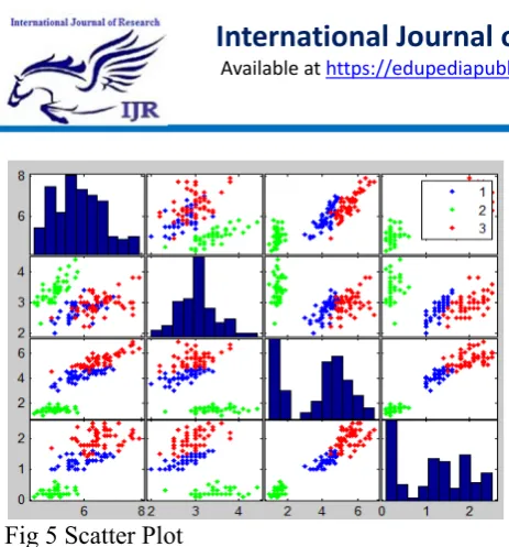
The Fisher-Iris dataset contains 150 instances of iris flowers collected in Hawaii. The dataset consists of 50 samples from each of three species of Iris (Iris setosa, Iris virginica and Iris versicolor). Four features were measured. The performance of algorithms will be evaluated according to the purity(P) and entropy(E) of the clustering results against the ground truth.
where r indicates the cluster index, k indicates the total number of classes in cluster r, nr indicates the number of elements in the cluster r, nir indicates the number of elements of class i inside the cluster r.
Experimental Summary on Fisher IRIS dataset
Algorithm Purity Entropy Time Mean Std Mean Std Mean Std PSC 79.90% 11.60% 0.31 0.11 3.90E-02 3.00E-04 m-PSC 88.60% 10.70% 0.32 0.09 3.80E-02 3.00E-04 Swarm RCE 95.80% 0.66% 0.15 0.02 9.50E-03 6.40E-05
MSEC 96.30% 0.51% 0.12 0.01 9.69E-01 4.38E-02
MSEC yields best purity relative to other algorithms. High purity is desirable for good cluster. But the high standard deviation shows that it is unstable.
Fig 1 Voronoi Cells Fig 2 Fuzzy Membership
Fig 5 Scatter Plot
V. Conclusion
Multi Swarm Based Ensemble Clustering (MSEC) preliminary experimental result on Benchmark dataset like Fisher-Iris dataset has shown promising results. Also MSEC reduces the memory and computational complexity and improves swarm diversity with the concept of charged particles.
In future, further work is to be done to improve MSEC stability, reliability and scalability for more complex datasets.
VI. References
[1] R. Eberhart and J. Kennedy. A new optimizer using particle swarm theory. In Proc. of the 6th International Symposium on Micro Machine and Human Science, pages 39–43, Oct. 4–6 1995.
[2] S. C. M. Cohen and L. N. de Castro. Data clustering with particle swarms. In Proc. of the 2006 IEEE Congress on Evolutionary Computation, pages 1792– 1798, Vancouver, 2006.
[3] P. Dayan, M. Sahani, and G. Deback. Unsupervised learning. In In The MIT Encyclopedia of the Cognitive Sciences. The MIT Press, 1999.
[4] A. Szabo, A. K. F. Prior, and L. N. de Castro. The proposal of a velocity memoryless clustering swarm. In Proc. of the 2010 IEEE Congress on Evolutionary Computation, pages 1–5, Barcelona, July 18–23 2010.
[5] A. K. Jain, M. N. Murty, and P. J. Flynn. Data clustering: A review. ACM Computing Surveys, 31(3):264–323, September 1999. ISSN 0360-0300. doi: 10.1145/331499.331504.
[6] Agbele, K., A. Adesina, D. Ekong and O.Ayangbekun. Stateof- the-art review on relevance of genetic algorithm to internet web search. Applied Computational Intelligence and Soft Computing, 25, 2012
[7]J. Kennedy and R. Eberhart. Particle swarm optimization. In Proceedings of the IEEE International Conference on Neural Networks, 1995., volume 4, pages 1942– 1948 vol.4, Nov 1995. doi: 10.1109/ICNN.1995.488968.
[8] S. C. M. Cohen and L. N. de Castro, “Data clustering with particle swarms,” in Proc. of the 2006 IEEE Congress on Evolutionary Computation, Vancouver, 2006, pp. 1792–1798.
the 2010 IEEE Congress on Evolutionary Computation, Barcelona, July 18–23 2010, pp. 1–5.
[10] M. Yuwono, S. Su, B. Moulton, and H. Nguyen, “Data clustering using variants of rapid centroid estimation,” IEEE Transactions on Evolutionary Computation, in press.
[11] A. Fred and A. Jain, “Combining multiple clusterings using evidence accumulation,” IEEE transactions on Pattern Analysis and Machine Intelligence, vol. 27, no. 6, pp. 835–850, 2005.
[12] Lourenco, A., Fred, "A. Comparison of Combination Methods using Spectral Clustering Ensembles," in Proc. Pattern Recognition on Information Systems, 2004, pp. 222-233.
[13] Fred A., Jain A. K., "Evidence accumulation clustering based on the k-means algorithm," in S.S.S.P.R, T.Caelli et al., editor,., Vol. LNCS 2396, Springer-Verlag, 2002, pp. 442 -451
[14] T. Wang, “Comparing hard and fuzzy c-means for evidence accumulation clustering,” in Proceedings of the 18th International Conference on Fuzzy Systems, ser. FUZZ-IEEE’09. Piscataway, NJ, USA: IEEE Press, 2009, pp. 468–473.
[15] T. Wang, “Ca-tree: A hierarchical structure for efficient and scalable co-association-based cluster ensembles,” Systems, Man, and Cybernetics, Part B: Cybernetics, IEEE Transactions on, vol. 41, no. 3, pp.
686–698, 2011.
[16] M. Yuwono, S. Su, B. Moulton, and H. Nguyen, “Data clustering using variants of rapid centroid estimation,” IEEE TRANSACTIONS ON EVOLUTIONARY COMPUTATION, VOL. 18, NO. 3, JUNE 2014
[17] M. Yuwono, S. W. Su, B. D. Moulton, and H. T. Nguyen. Fast unsupervised learning method for rapid estimation of
cluster centroids. In Proc. of the 2012 IEEE Congress on Evolutionary Computation, pages 889–896, June 10–15 2012.
[18] M. Yuwono, S. W. Su, B. D. Moulton, and H. T. Nguyen. Optimization strategies for rapid centroid estimation. In Proc. of the 34rd Annual International Conference of the IEEE EMBS, pages 6212–6215, San Diego, Aug. 28–sept. 1 2012.
[19] M. Yuwono, S. W. Su, B. D. Moulton, and H. T. Nguyen. Method for increasing the computation speed of an unsupervised learning approach for data clustering. In Proc. of the 2012 IEEE Congress on Evolutionary Computation, pages 2957– 2964, June 10–15 2012.
[20] L. Vendramin, R. J. G. B. Campello, and E. R. Hruschka, “On the comparison of relative clustering validity criteria.” in SIAM International Conference on Data Mining, 2009, pp. 733–744.
[21] J. Bezdek and N. Pal, “Some new indexes of cluster validity,” IEEE Transactions on Systems, Man, and Cybernetics, Part B: Cybernetics, vol. 28, no. 3, pp. 301–315, 1998.