Micro-Processor based Improved
Ultrasonic
Direction and Range Finder
Ariel Barzilay, Arieh Salomon, Dov Avraham and Zeev Zalevsky
School of Engineering, Bar-Ilan University, Ramat-Gan 52900, Israel
Abstract
—
This document gives formatting instructions for authors preparing papers for publication in the Proceedings of an IEEE conference. The authors must follow the instructions given in the document for the papers to be published. You can use this document as both an instruction set and as a template into which you can type your own text. In this paper we present a novel microprocessor based improved ultrasonic direction and range finder combining both extended operational range as well as improved sensing resolution. The improved range related performance includes minimal measurement range of only few centimeters while the maximal range can be hundreds of meters and even more than that. The obtained measurement accuracy is 1.5cm and the range resolution is 1mm. The measurements can be performed in 3-D space.Keywords— ultrasound, range finder, direction finder
I. INTRODUCTION
Sensing of distance to objects using ultra sound is a well known technique [1,2]. However the commonly available such measuring devices which are small and low price either perform the measurement in 1-D space or have limited measurement range being expressed in too large minimal range and too short maximal range. They also have low accuracy and resolution [3-6].
As a comparison one may see table 1 where two common range finder devices are exhibited in the left and central column of the table. For comparison, the experimentally validated performance using the constructed device described in this paper is presented in the right column. One may see that the constructed device exhibits both very short minimal measurement range of only few centimeters as well as very large maximal range that can be hundreds of meters and even more (although the experimental measurements were limited to about 9-10m since they were performed in the lab). It has very high precision of 1.5cm and measuring spatial resolution of only 1mm. In addition, the constructed device can perform 3-D measurement rather than a 1-D and thus it may be used not only for range estimation but also for direction finding.
The significant improvement in performance is obtained by special trilateration [7-10] based algorithm that was developed and implemented on ADuC841 microprocessor. This paper presents the construction and the experimental laboratory validation of the constructed prototype as well as its experimental comparison to other available modules.
In section 2 we give the theoretical background for the developed algorithmic. In section 3 we described the constructed prototype. Section 4 deals with the experimental validation of the constructed module. The paper is concluded in section 5.
TABLEI
COMPARISON OF PERFORMANCE BETWEEN TWO COMMONLY USED RANGE FINDERS (LEFT AND CENTRAL COLUMN) AND THE CONSTRUCTED PROTOTYPE
(RIGHT COLUMN).
II. THEORETICAL BACKGROUND
The simplest relation between sound power level and sound pressure level is found for a free-field, non-directional sound source, as given by the following equation [11]:
10 10
20
log
10log
P W r Q K T
L
L
(1)where Lp is the sound pressure level (in dB units) in
comparison to reference level of 20µPa, Lw is the sound power
with air at or near standard conditions, T is usually negligible and therefore equals to 0. Q is the directivity factor.
The relation between sound power level and sound pressure level can be obtained in a different way as:
2 10 4 10 4 log p W Q A L L r
(2)
where A is the total absorption area in the room in units of m2.
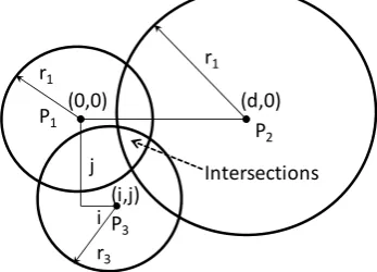
Trilateration [7,8] is a method for determining the intersections of three spheres’ surfaces given the centers and radii of the three. More generally, trilateration methods involve the determination of absolute or relative locations of points by measurement of distances, using the geometry of spheres or triangles. In contrast to triangulation it does not involve the measurement of angles. Trilateration is mainly used in surveying and navigation, including global positioning systems (GPS) [9].
In a 2-D plane using two reference points is normally sufficient to leave only two possibilities for the extracted location while addition of a third reference point or other apriori known information may resolve this ambiguity. In 3-D space, using three reference points similarly leaves only two possibilities and the ambiguity is resolved by the addition of a fourth reference point or other apriori information.
The solution is found by formulating the equations for the three spheres’ surfaces and then solving the three equations for the three unknowns x, y, and z which are the coordinates of the object that is to be allocated. To simplify the calculations, the equations are formulated so that the centers of the spheres are on the z=0 plane. Also the formulation is such that one center is at the origin, and one other is on the x-axis. It is possible to formulate the equations in this manner since any three non-colinear points lie on a plane. After finding the solution it can be transformed back to the original three dimensional Cartesian coordinates system.
In Fig. 1 one may see a schematic explanation for the trilateration approach. (0,0) P1 r1 (d,0) P2 r1 r3 (i,j) j
i P3
Intersections
Fig. 1: The schematic explanation for the trilateration approach.
In plane z=0 one may see the 3 spheres’ centers, P1, P2, and P3; their x, y coordinates; and the 3 spheres’ radii, r1, r2 and r3. The two intersections of the three spheres’ surfaces are directly in front and directly behind the point of designated intersections in the z=0 plane.
The equations for the three spheres are:
2
2 2 2
1 x y z
r
2 2
2 2
2
(
x d
)
y
z
r
2 2
2 2
3 (x i) (y j) z
r (3)
To solve those equations one needs to find a point located at (x, y, z) that satisfies all the three of them. First we subtract the second equation from the first and solve for x:
2 2 2
( 1 2 ) / 2
x
r
r
d
d(4)
We assume that the first two spheres intersect in more than one point, i.e. d-r1 < r2 < d+r1. In this case substituting the
equation for x back into the equation for the first sphere produces the equation for a circle, the solution to the intersection of the first two spheres is:
2
2 2 2 2 2 2 2
/ 4 1 ( 1 2 )
y z r r r d d (5)
Substituting
2
2 2 2 2 2 2 2
/ 4 1 ( 1 2 )
y z r r r d d (6)
into the formula for the third sphere and solving for y results with:
2 2
2 2
2 2 2 2 2 2 2
( 1 3 ) / 2 / ( 1 3 ) / 2 (( 1 2 ) / 2 ) /
y r r ij j ix j r r ij j i r r d d j
(7) Now that we have the x- and y-coordinates of the solution point, we can simply rearrange the formula for the first sphere to find the z-coordinate:
2 2
2 2 2 2 2 2 2 2
2 2 2
(
1 (1 2 )/2 ) ((1 3 )/2 ((1 2 )/2 )/ )
z r r r d d r r ij j i r r d d j (8) An easy way to comply with the conference paper formatting requirements is to use this document as a template and simply type your text into it.
III.THE CONSTRUCTED PROTOTYPE
The scheme of the transmission system (input/output) is presented in Fig. 2. It includes the ADuC841 microprocessor output which is 8 triangles waves that are repeatedly being sent at frequency of 40KHz. Those waves are being input to the ultrasonic transmitter and converted into 40KHz ultrasonic waves propagating in free space.
Fig. 2: The scheme of the transmission system (input/output).
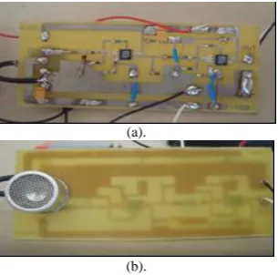
(a).
(b).
Fig. 3: The photos of one out of the three amplification kits assembling the receiving system. The ultrasonic sensor is welded to the input: (a). Front. (b). Back.
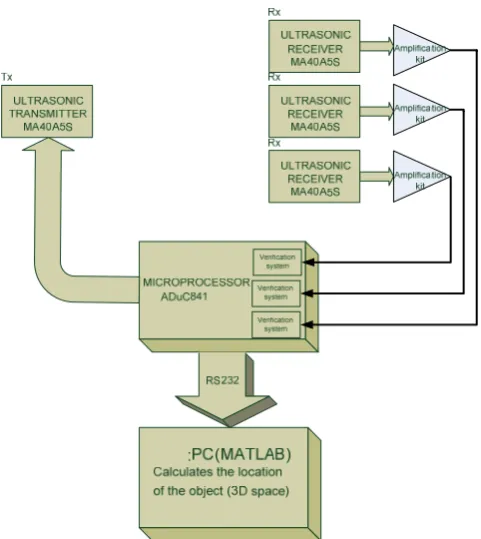
The full scheme of the receiving system is presented in Fig. 4 where the outputs of the three receivers are being amplified using the amplification kits by a factor of 10,000 and then input to proper inputs of the ADuC841 microprocessor.
Fig. 4: The scheme of the receiving system (input/output).
After receiving an indication that acoustic waves have been received in the receiving system and after measuring the propagation time in the free-field, we are sending the information to the data processing system to calculate the location of the object in a 3-D space. Parts of the data processing system were realized using the ADuC841 microprocessor. The full scheme of the constructed system may be seen in Fig. 5.
Fig. 5: The full scheme of the constructed system.
Let us now describe the flow chart of the proposed ultrasonic range finder (see Fig. 6). Basically, the ultrasonic range finder flowchart consists of two main blocks:
1) Microprocessor ADuC841 block. 2) Matlab block (run on a PC).
Fig. 6: The flow chart of the proposed ultrasonic range finder.
The connection between the microprocessor ADuC841 block and the Matlab block is accomplished by using RS-232 (Recommended Standard 232). RS-232 is a standard communication format for serial binary single-ended data and control signals connecting between a DTE (Data Terminal Equipment) and a DCE (Data Circuit-terminating Equipment).
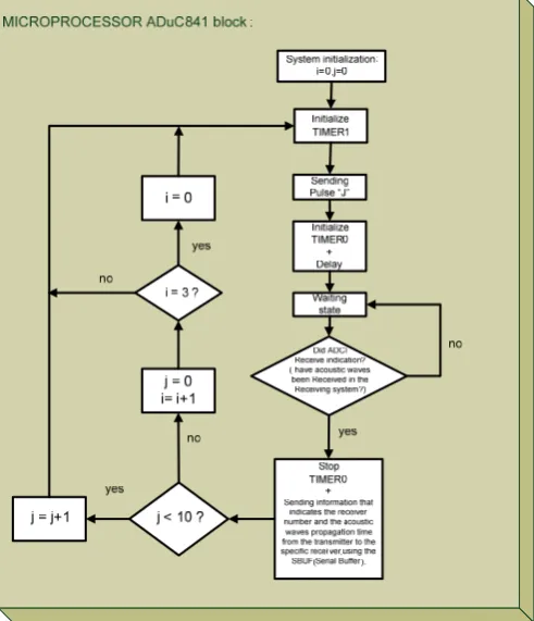
Fig. 7: The flow chart of the microprocessor ADuC841 block.
In the constructed module we used ADC0/ADC1/ADC2 channels. i: stands for the relevant ADC number(0/1/2). j: stands for the number of the pulse being sent. Every pulse consists of 8 triangle waves. Amplitude: 5V; Nominal frequency of 40KHz. The pulses repeatedly being sent after receiving an indication that acoustic waves have been received in the receiving system. TIMER0 is one of the ADuc841 microprocessor timers. The timer is used for measuring the acoustic wave’s propagation time in free-field. TIMER1 is one of the ADuc841 microprocessor timers. The timer enables us to get 8 triangle waves at frequency of 40KHz. With the assistance of RS232 we are sending the time measurements (serial communication) from the ADuC841 microprocessor to the PC (Matlab code).
Fig. 8: The flow chart of the Matlab block.
The Matlab block that is responsible for the algorithmic procedure, that eventually evaluates the direction and the range to the inspected object, is described in Fig. 8.
Fig. 9: The overall block diagram of the proposed ultra sonic range finder.
In Fig. 10 we present the timing diagram of the system. The sonar system is a synchronic system. This means that it depends on the timing signals of the microprocessor’s clock whose working frequency is 11.0592MHz (temporal period of T0.0904
s). When the system initializes, transmitting-receiving periods start running and are timed according to this clock. A transmitting-receiving period starts when electrical pulses are transmitted from the ultrasonic transmitter and it stops when acoustic signals are received in the 3 receivers. This completes the receiving process.(a).
(b).
Fig. 10: Timing diagram. (a). Two transmitting-receiving periods. (b). Two transmitting-receiving periods (lower resolution). Every transmit-receive loop is represented as one delta pulse.
Time Algorithm (see Fig. 10(a)):
1.1. The microprocessor creates electrical pulses that are characterized as eight consecutive triangle waves at frequency of 40KHz (ultrasonic).
1.2. After the transmission of the pulses, we allow interrupts from TIMER0. This timer measures the
time that it took the acoustic waves to reach the receiving system from the moment they were transmitted. We also raise the EADC flag in order to allow ADC (Analog to Digital Converter) interruptions. The electrical signals that were received in the output of the amplification kits are sent back to the microprocessor to “Verify Indication” which is a program based application that differentiates between acoustic signals and other environmental noises. 1.3. When indication has been verified (indication flag is
raised), we stop TIMER0 and restart its value to 0 to allow the next measurement. At this time, the EADC flag is also zeroed in order to allow us to process the data without any ADC interruptions. This flag is raised after the next transmission.
1.4. The data that we received includes the receiver (amplification kit), index (1, 2 or 3), and the number of TIMER0 interruptions. It is sent to the data processing unit (Matlab application). New transmitting-receiving period starts.
In Fig. 10(b) one may see two transmitting-receiving periods (lower resolution). Every transmit-receive loop is represented as one delta pulse.
Time Algorithm (see Fig. 10(b)):
2.1. ADC0 channel is enabled. 2.2. First transmit-receive loop starts.
2.3 After 10 periods (of transmit-receive loop), ADC0 channel is disabled and ADC1 channel is enabled.
2.4 After 10 periods, ADC1 channel is disabled and ADC2 channel is enabled.
2.5. After 10 periods, ADC2 channel is disabled and ADC0 channel is enabled.
2.6. Items 2.3–2.5 repeat themselves periodically.
IV.EXPERIMENTAL VALIDATION
The first measurement analysis with the constructed prototype included the following measurements: The transmitter coordinates (X, Y, Z) were (1.08, 0.31, 2.25) in meter units. The transmitter coordinates (X, Y, Z) as received in the first system measurement were (1.0904, 0.3291, 2.2527).
Fig. 11: The scope photo for the first measurement analysis.
respectively. In Fig. 11 we present the scope photo for the first measurement analysis.
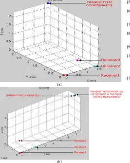
In the second measurement receiver1, receover2 and receiver3 (X, Y, Z) coordinates (m) were (0, 0, 0), (1.5, 0, 0) and (1.36, 0.9, 0) respectively. The distance between receiver1 and receiver2 was 1.5m.
The transmitter coordinates (X, Y, Z) were (1.66, 3.16, 2.27). The transmitter coordinates (X, Y, Z), as received in the second system measurement were (1.6725, 3.1775, 2.2547). Thus, the percentage relative errors for transmitter X(m), Y(m) and Z(m) coordinates were 0.75%, 0.55% and 0.67% respectively. The graphical representation of the second measurement may be seen in Fig. 12(a).
In the third measurement receiver1, receover2 and receiver3 (X, Y, Z) coordinates (m) were (0, 0, 0), (2, 0, 0) and (1.5, 2, 0) respectively. The distance between receiver1 and receiver2 was 2m.
The transmitter coordinates (X, Y, Z) were (7.65, 0.86, 3.61). The transmitter coordinates (X, Y, Z), as received in the second system measurement were (7.8031, 0.8734, 3.6292). Thus, the percentage relative error errors for transmitter X(m), Y(m) and Z(m) coordinates were 2%, 1.56% and 0.53% respectively. The graphical representation of the third measurement may be seen in Fig. 12(b).
(a).
(b).
Fig. 12: Graphical representation of: (a). The second measurement. (b). The third measurement.
V. CONCLUSIONS
In this paper we present the description of an ultrasonic range/direction finding system, with high accuracy and improved resolution and working range, that was constructed and experimentally validated in our lab.
The sonar system is based on finding object’s location by using a transmitter and three ultrasonic receivers, ADuC841 microprocessor and the Matlab language programming (run over a PC).
The ultrasonic transmitter transmits acoustic waves that propagate in a free-field. After the acoustic waves have been received by each one of the receivers, we can find the object’s location in a 3-D space by measuring the waves’ propagation time and calculating the waves’ velocity (trilateration method).
REFERENCES
[1] F. Massa, "Ultrasonics in Industry," Fiftieth Anniversary Issue, Proc IRE (1992).
[2] D. P. Massa, “Choosing an Ultrasonic Sensor for Proximity or Distance Measurement,” Sensor Magazine (1999).
[3] http://www.robot-electronics.co.uk/htm/srf05tech.htm
[4] M. Minami, Y. Fukuju, K. Hirasawa, S. Yokoyama, M. Mizumachi, H. Morikawa and T. Aoyama, “DOLPHIN: A Practical Approach for Implementing a Fully Distributed Indoor Ultrasonic Positioning System,” UbiComp 2004: Ubiquitous Computing 3205/2004, 347-365 (2004).
[5] C. Randell and H. Muller, “Low Cost Indoor Positioning System,” Ubicomp 2001: Ubiquitous Computing 2201/2001, 42-48 (2001). [6] M. Riccabona, T. R. Nelson, D. H. Pretorius, “Three-dimensional
ultrasound: accuracy of distance and volume measurements,” Ultrasound in Obstetrics and Gynecology 7, 429-434 (2003).
[7] F. Thomas and L. Ros, “Revisiting trilateration for robot localization,” IEEE Transactions on Robotics 21, 93–101 (2005).
[8] J. Borenstein, H. R. Everett, L. Feng and D. Wehe, “Mobile robot positioning: Sensors and techniques,” Journal of Robotic Systems 14, 231-249 (1998).
[9] M. Brain and T. Harris, “How GPS receivers work,” http://www.howstuffworks.com/gps1.htm.
[10] N. Bulusu, D. Estrin, L. Girod and J. Heidemann, “Scalable Coordination for wireless sensor networks: Self-Configuring Localization Systems,” In Proceedings of the Sixth International Symposium on Communication Theory and Applications (ISCTA 2001), Ambleside, Lake District, UK (July 2001).