Impact of the Test Device on the Behavior of the
Acoustic Emission Signals: Contribution of the
Numerical Modeling to Signal Processing
Oumar Issiaka Traore, Paul Cristini, Nathalie Favretto-Cristini, Laurent Pantera and Sylvie Viguier-Pla.
Abstract—In a context of nuclear safety experiment monitoring with the non destructive testing method of acoustic emission, we study the impact of the test device on the interpretation of the recorded physical signals by using spectral finite element modeling. The numerical results are validated by comparison with real acoustic emission data obtained from previous ex-periments. The results show that several parameters can have significant impacts on acoustic wave propagation and then on the interpretation of the physical signals. The potential position of the source mechanism, the positions of the receivers and the nature of the coolant fluid have to be taken into account in the definition a pre-processing strategy of the real acoustic emission signals. In order to show the relevance of such an approach, we use the results to propose an optimization of the positions of the acoustic emission sensors in order to reduce the estimation bias of the time-delay and then improve the localization of the source mechanisms.
Index Terms—Acoustic Emission, Reactivity Initiated Accident, Spectral Finite Element Modeling
I. INTRODUCTION
R
EACTIVITY Initiated Accident (RIA) is a nuclear reac-tor accident that involves an unexpected and very fast increase in fission rate and reactor power due to the ejection of a control rod. The power increase may damage the fuel clad and the fuel pellets of the reactor. The French Alternative Energies and Atomic Energy Commission (CEA) operates a pool-type reactor dedicated to fuel behavior study in RIA conditions. During the experiments, several non-destructive methods are used to inspect the reactor and to get information on the behavior of the fuel clad and the fuel pellet. Among them the acoustic emission (AE) technique is of major interest. It has the advantage of being simple to adapt to nuclear-oriented purposes and allows a quasi-real-time monitoring of the experiment [1]–[5]. One goal of the AE testing is to process the AE signals in such a way that they can be associated with specific physical source mechanisms occurring in the tested structure or material. In most of the applications, the starting point of this processing is to clean as much as possible the received signal from the potential bias introducedOumar Issiaka Traore, Paul Cristini and Nathalie Favretto-Cristini are with Aix-Marseille Univ., CNRS, Centrale Marseille, LMA, France (Email: [email protected], [email protected], [email protected])
Laurent Pantera is with CEA, DEN, DER/SRES, Cadarache,F13108 Saint-Paul-Lez-Durance, France (Email: [email protected])
Sylive Viguier-Pla is with Université de Perpignan via Domitia, LAMPS, 52 av. Paul Alduy, 66860 Perpignan Cedex 9, France and Université Paul Sabatier, 118 Route de Narbonne, F-31062 Toulouse Cedex 9, France
by several parameters among which the choice and the setting of the AE sensors [6], [7], the environmental noise, the wave propagation path in the structure and the signals acquisition system.
Depending on the stochastic behavior of noise, several denoising methods exist in order to cope with the environmental noise [8]–[10]. In most of the cases, the transfer functions associated with the sensor and the acquisition system are known, a simple deconvolution is then enough to remove their impacts [11]. In the case of the wave propagation path, except in some rare cases (e.g. homogeneous media), the correction of its impact on the received signal is a complex problem. For instance, when the structure is complex such as the test device of a nuclear safety experiment reactor, the potential impacts of several parameters have to be taken into account, making difficult the estimation of the transfer function by experimental methods. Other tools like analytical computations or numerical simulations then become interesting alternatives to experimental methods. Indeed, contrary to experimental methods, they can easily integrate potential changes of the position of the source mechanism (so of the transfer function) and then the impact of these changes on the transfer function.
The main objective of this article is to use the numerical modeling in the particular case of RIA experiments in order to explore different scenarios of wave propagation in test device and compare the associated transfer functions. In addition, we also study the impact of a change of the heat transfer fluid (sodium or pressurized water) and the impact of changes of the positions of the AE sensors.
In the second section, we present and study the environment of the RIA experiment with a focus on the test device. Its geometry and configuration are studied in order to get a simplified problem. The third section is devoted to the numerical modeling of the test device by using a spectral finite element method. The obtained numerical signals are analyzed and the impacts of the position of the source mechanisms, of the position the sensors and of a change of coolant fluid are studied. In the last section, we discuss the results and analyze their impact on the experimental protocol.
II. DESCRIPTION OF THE TEST DEVICE
ofU O2rods and specially designed to support an injection of
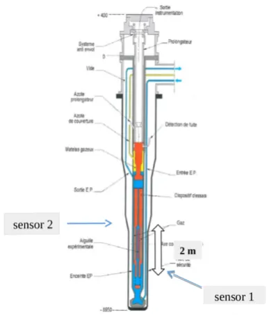
reactivity. The reactor includes an experimental loop specially designed to receive in the center of the driver core the instrumented test device housing the fuel rod to be tested. This test device is equipped with several sensors (including two piezoelectric AE sensors or microphones) to control the experiment and to characterize the behavior of the fuel rod during the power burst. These sensors are made of lithium niobate cristal with a pass-band of 5-400 kHz and designed to work in nuclear harsh environment up to 600 degrees Celsius. They are located at the top and the bottom of the fuel rod, respectively, and are distant of 2 m (Fig. 1). A (40 dB) preamplifier is associated with each sensor. The sampling rate is 2.5µs.
Figure 1: Illustrative picture of the complete test device with the positions of the two AE sensors
In such a context, we recorded the operating noise of the reactor during an experiment realized in 1997. The acquired signal and its spectrum are shown in Fig. 2. It can be observed a very strong component around the frequency of
180 kHz. As this signal is observed before the power burst, this 180 kHz component cannot correspond to a physical
mechanism. However, it is present during all the experiment and biases the interpretation of the signals corresponding to source mechanisms. Then, it is of crucial importance to identify its origin in order to remove it in future experiments. The deterministic character of this180kHzcomponent makes
us think that it can be associated with an environmental noise or with an impulse response of the test device but it is impossible to determine its origin only from data-processing. This is a typical example of a problem which can be addressed with numerical modeling. In this case, we guess that it will provide new insights that will help us to determine the origin of this strong frequency component.
Figure 2:Example of operating noise of the reactor recorded during an experiment realized in 1997. Signal recorded at the second sensor (top) and its spectrum (bottom)
III. MODELING OF WAVE PROPAGATION ON THE TEST DEVICE
As it is impossible to model the test device with all its complexity we chose to focus on a 3m long region which
includes the positions of two AE sensors and the fuel rod to be tested. This limited domain is sufficient to study the wave propagation path from the potential positions of source mechanisms to the receivers. It corresponds to a stratified cylinder with eight layers of different types of media (cf. Fig. 3 and 4). Due to the presence of a Xenon layer (a neutron absorber) which has a much smaller impedance value than other layers, it is not necessary to consider wave propagation above this layer. We finally end up with a simplified model depicted in Fig. 4 whose physical characteristics are given in Table I.
Uranium Zircaloye Sodium Xenon Molybdenum Niobium Zirconium Uranium Zircaloye Sodium Xenon Molybdenum Niobium Zirconium Uranium Zircaloye Sodium Xenon Molybdenum Niobium Zirconium Uranium Zircaloye Sodium Xenon Molybdenum Niobium Zirconium Uranium Zircaloye Sodium Xenon Molybdenum Niobium Zirconium Uranium Zircaloye Sodium Xenon Molybdenum Niobium Zirconium Uranium Zircaloye Sodium Xenon Molybdenum Niobium Zirconium Uranium Zircaloye Sodium Xenon Molybdenum Niobium Zirconium Uranium Zircaloye Sodium Xenon Molybdenum Niobium Zirconium
Figure 3: Radial section of the test device at z = 0. Illustration
of the different types of media constituting the cylinder. Note that the number and the type of the layers can change depending on the
position on thez−axis.
17.2 mm
3 m
Oz : 1 cm = 2,15 mm Or : 1 cm= 0,12 m = 120 mm
Or Oz
Sodium Stainless steel
Uranium Zircaloye
Figure 4: Longitudinal section of the simplified test device of3m
of length and17.2mmof width.
Table I: Density and wave speeds for layers and materials associated with the simplified test device
Media ρ(Kg/m3) c
l(m/s) ct(m/s) Uranium 11000 3370 2020 Zircaloy 6500 4720 2360 Inox 7900 5460 3070
Sodium 968 2300
-Water 1000 1436
-Xenon 6 1090
-For the sake of simplicity, we consider an axysimmetric model (with respect to thez−axis), which simplifies greatly
the computations.
A. Brief overview on the chosen numerical tools
The spectral-element method belongs to the finite-element family of methods. It was initially developed for fluid me-chanics [12] and is now commonly used for the solution of elastodynamics problems [13], [14]. It combines the accuracy of a pseudo spectral method with the flexibility of a finite-element method.
All numerical simulations were performed with the open-source SPECFEM2D software and meshes of the simplified model were performed with the GMSH software[15], [16]. One advantage of this numerical model is that it works in the time-domain. Among all the futures provide by the SPECFEM2D software, the possibility of generating source signal with a very wide-band spectrum analogous to a Dirac delta function is very attractive. It allows the generation of transfer functions from the source to the different receiver
positions. It is thus possible to compare the results obtained from numerical simulations with experimental acquisitions.
B. Results Analysis
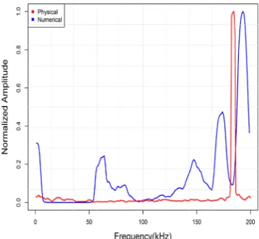
Fig. 5 shows the superposition of the normalized spectrum of the operating noise depicted in the Fig. 2 and of the transfer function of the test device with a source located on the fuel clad. We recover, with a slight shift toward high frequencies, the very strong frequency component around180kHzwhich
has been observed in the experimental data (cf. Fig. 5). It can then be concluded that the origin of this frequency peak is associated with a resonance of the structure of the test device.
Figure 5: Superposition of the normalized spectra of the operating noise of the reactor (red) and of the transfer function of the test device associated with a source located on the fuel clad (blue)
In the following, we will use only use a Dirac type source. This allows to get the transfer functions associated with different combinations of source and sensors positions and then to analyze the impact of the position of the source mechanism (respectively of the receiver) on the physical signals. Note that the temporal signals corresponding to the spectra which will be depicted in the following have been normalized.
ofU O2rods and specially designed to support an injection of
reactivity. The reactor includes an experimental loop specially designed to receive in the center of the driver core the instrumented test device housing the fuel rod to be tested. This test device is equipped with several sensors (including two piezoelectric AE sensors or microphones) to control the experiment and to characterize the behavior of the fuel rod during the power burst. These sensors are made of lithium niobate cristal with a pass-band of 5-400 kHz and designed to work in nuclear harsh environment up to 600 degrees Celsius. They are located at the top and the bottom of the fuel rod, respectively, and are distant of 2 m (Fig. 1). A (40 dB) preamplifier is associated with each sensor. The sampling rate is 2.5µs.
Figure 1: Illustrative picture of the complete test device with the positions of the two AE sensors
In such a context, we recorded the operating noise of the reactor during an experiment realized in 1997. The acquired signal and its spectrum are shown in Fig. 2. It can be observed a very strong component around the frequency of
180 kHz. As this signal is observed before the power burst, this 180 kHz component cannot correspond to a physical
mechanism. However, it is present during all the experiment and biases the interpretation of the signals corresponding to source mechanisms. Then, it is of crucial importance to identify its origin in order to remove it in future experiments. The deterministic character of this180kHzcomponent makes
us think that it can be associated with an environmental noise or with an impulse response of the test device but it is impossible to determine its origin only from data-processing. This is a typical example of a problem which can be addressed with numerical modeling. In this case, we guess that it will provide new insights that will help us to determine the origin of this strong frequency component.
Figure 2:Example of operating noise of the reactor recorded during an experiment realized in 1997. Signal recorded at the second sensor (top) and its spectrum (bottom)
III. MODELING OF WAVE PROPAGATION ON THE TEST DEVICE
As it is impossible to model the test device with all its complexity we chose to focus on a 3m long region which
includes the positions of two AE sensors and the fuel rod to be tested. This limited domain is sufficient to study the wave propagation path from the potential positions of source mechanisms to the receivers. It corresponds to a stratified cylinder with eight layers of different types of media (cf. Fig. 3 and 4). Due to the presence of a Xenon layer (a neutron absorber) which has a much smaller impedance value than other layers, it is not necessary to consider wave propagation above this layer. We finally end up with a simplified model depicted in Fig. 4 whose physical characteristics are given in Table I.
Uranium Zircaloye Sodium Xenon Molybdenum Niobium Zirconium Uranium Zircaloye Sodium Xenon Molybdenum Niobium Zirconium Uranium Zircaloye Sodium Xenon Molybdenum Niobium Zirconium Uranium Zircaloye Sodium Xenon Molybdenum Niobium Zirconium Uranium Zircaloye Sodium Xenon Molybdenum Niobium Zirconium Uranium Zircaloye Sodium Xenon Molybdenum Niobium Zirconium Uranium Zircaloye Sodium Xenon Molybdenum Niobium Zirconium Uranium Zircaloye Sodium Xenon Molybdenum Niobium Zirconium Uranium Zircaloye Sodium Xenon Molybdenum Niobium Zirconium
Figure 3: Radial section of the test device at z = 0. Illustration
of the different types of media constituting the cylinder. Note that the number and the type of the layers can change depending on the
position on thez−axis.
17.2 mm
3 m
Oz : 1 cm = 2,15 mm Or : 1 cm= 0,12 m = 120 mm
Or Oz
Sodium Stainless steel
Uranium Zircaloye
Figure 4: Longitudinal section of the simplified test device of3m
of length and17.2mmof width.
Table I: Density and wave speeds for layers and materials associated with the simplified test device
Media ρ(Kg/m3) c
l(m/s) ct(m/s) Uranium 11000 3370 2020 Zircaloy 6500 4720 2360 Inox 7900 5460 3070
Sodium 968 2300
-Water 1000 1436
-Xenon 6 1090
-For the sake of simplicity, we consider an axysimmetric model (with respect to thez−axis), which simplifies greatly
the computations.
A. Brief overview on the chosen numerical tools
The spectral-element method belongs to the finite-element family of methods. It was initially developed for fluid me-chanics [12] and is now commonly used for the solution of elastodynamics problems [13], [14]. It combines the accuracy of a pseudo spectral method with the flexibility of a finite-element method.
All numerical simulations were performed with the open-source SPECFEM2D software and meshes of the simplified model were performed with the GMSH software[15], [16]. One advantage of this numerical model is that it works in the time-domain. Among all the futures provide by the SPECFEM2D software, the possibility of generating source signal with a very wide-band spectrum analogous to a Dirac delta function is very attractive. It allows the generation of transfer functions from the source to the different receiver
positions. It is thus possible to compare the results obtained from numerical simulations with experimental acquisitions.
B. Results Analysis
Fig. 5 shows the superposition of the normalized spectrum of the operating noise depicted in the Fig. 2 and of the transfer function of the test device with a source located on the fuel clad. We recover, with a slight shift toward high frequencies, the very strong frequency component around180kHzwhich
has been observed in the experimental data (cf. Fig. 5). It can then be concluded that the origin of this frequency peak is associated with a resonance of the structure of the test device.
Figure 5: Superposition of the normalized spectra of the operating noise of the reactor (red) and of the transfer function of the test device associated with a source located on the fuel clad (blue)
In the following, we will use only use a Dirac type source. This allows to get the transfer functions associated with different combinations of source and sensors positions and then to analyze the impact of the position of the source mechanism (respectively of the receiver) on the physical signals. Note that the temporal signals corresponding to the spectra which will be depicted in the following have been normalized.
Figure 6:Illustration of the impact of the position of the source on the transfer function of the test device. Spectra of transfer functions associated with different positions of the source.
Figure 7:Illustration of the impact of the position of the receiver on the transfer function of the test device. Spectra of transfer functions associated with different positions of source and receiver.
We notice that these results are consistent from a theoretical point of view. Indeed, the test device being a stratified media, moving the position of the source mechanism (respectively of the receiver) from a layer to another leads to change the wave propagation path and then of the excitation of the resonant frequencies.
1) Detailed analysis of the transfer functions for different frequency ranges: Let us consider a source located at three different positions (bottom, middle and top) in the second layer associated with the fuel clad. Analysis of the spectra of the recorded transfer functions in the frequency range
[0,200] kHz highlights two interesting results (cf. Fig. 8). First, we observe that up to80kHz the transfer functions are quasi-constant. Thus, for source mechanisms situated in this layer (e.g. clad failures), there is no significant impact of the test device. Second, whatever the position of the sensor, we observe a peak of energy around 180kHz (more pronounced on sensor 2) associated with a resonant frequency of the test device (cf. Fig 5). This peak is not observed when sources are located in other layers indicating that the associated resonance is strongly connected to the structure of the fuel/clad couple.
Figure 8: Focus on the spectra associated with different positions of the source in the frequency range [0,200]kHz.
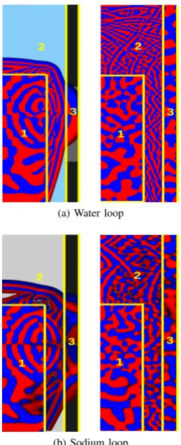
2) Impact of a change of heat transfer fluid: For visu-alization purposes, we increase the sizes of the simplified model so that we are able to identify how the acoustic energy is distributed into the model. Three zones can be identified (cf. Fig. 9) independently of the nature of the heat transfer fluid. Nevertheless, it can be noticed that the oscillations present in zone 2 corresponding to the fluid part have a much higher frequency content with a water loop than with a sodium loop.
(a) Water loop
(b) Sodium loop
Figure 9:Snapshots of wave propagation with two different coolant fluids.
IV. DISCUSSIONS AND CONCLUSION
The objective of this article was to use numerical modeling to analyze the impact of the structure of the test device on recorded physical AE signals in the case of RIA experiments. A resonant frequency of the test device observed in physical signals has been identified with the help numerical compu-tations. This resonant frequency being only connected to the structure of the test device, it can be removed safely from recorded signals, making their interpretation more effective. The results we obtained showed that there is a strong depen-dence of the transfer function on the source/receiver relative positions. It is thus impossible to define a global transfer function. We also conclude that it is not possible to use classical deconvolution methods when the source position is unknown. Additionally, numerical simulations suggests that frequencies up to 80 kHz have to be preferred because of the flat response of the transfer functions in this frequency band. No perturbation on the signal coming from the structure of the test device should be expected in this frequency band. A perspective of this work which is a direct consequence of the feasibility of performing numerical computations is the possibility of optimizing the receiver positions. From the previous results, we can assert that AE sensors should always be located before the Xenon layer and should be put at the same distance from the z − axis. This would reduce the estimation bias of the time-delay between the two AE sensors and then improve the source mechanism localization.
REFERENCES
[1] SP. Ying. The use of acoustic emission for assessing the integrity of a nuclear reactor pressure vessel. NDT International, 12(4):175–179, 1979.
[2] P. Runow. The use of acoustic emission methods as aids to the structural integrity assessment of nuclear power plants. International Journal of Pressure Vessels and Piping, 21(3):157–207, 1985.
[3] Q. Ai, C. Liu, X. Chen, P. He, and Y. Wang. Acoustic emission of fatigue crack in pressure pipe under cyclic pressure. Nuclear Engineering and Design, 240(10):3616–3620, 2010.
[4] L. Hégron, P. Sornay, and N. Favretto-Cristini. Compaction of a bed of fragmentable particles and associated acoustic emission. IEEE Transactions on Nuclear Science, 61(4):2175–2181, 2014.
[5] N. Favretto-Cristini, L. Hégron, and P. Sornay. Identification of the fragmentation of brittle particles during compaction process by the acoustic emission technique.Ultrasonics, 67:178–189, 2016. [6] J. Roget.Essais non destructifs: L’émission acoustique: Mise en oueuvre
et applications. AFNOR; CETIM, 1988.
[7] G. Gautschi.Piezoelectric sensorics: force, strain, pressure, acceleration and acoustic emission sensors, materials and amplifiers. Springer Science & Business Media, 2002.
[8] O.I. Traoré, L. Pantera, N. Favretto-Cristini, and S. Viguier-Pla. Emis-sion acoustique et traitement du bruit : cas de signaux expérimentaux en contexte nucléaire. In13e Congrès Français d’Acoustique, CFA 2016, Le Mans, France, April 2016.
[9] O.I. Traore, L. Pantera, N. Favretto-Cristini, P. Cristini, S. Viguier-Pla, and P. Vieu. Structure analysis and denoising using singular spectrum analysis: application to acoustic emission signals from nuclear safety experiments. Measurement, 104:78 – 88, 2017.
[10] V. Barat, Y. Borodin, and A. Kuzmin. Intelligent acoustic emission signal filtering methods.Journal of Acoustic Emission, 28:109–119, 2010. [11] C. U. Grosse and M. Ohtsu.Acoustic emission testing. Springer Science
& Business Media, 2008.
[12] Y. Maday and A.T. Patera. Spectral element methods for the in-compressible navier-stokes equations. In IN: State-of-the-art surveys on computational mechanics (A90-47176 21-64). New York, American Society of Mechanical Engineers, 1989, p. 71-143. Research supported by DARPA., pages 71–143, 1989.
[13] D. Komatitsch. Spectral and spectral-element methods for the 2D and 3D elastodynamics equations in heterogeneous media. Theses, Institut de physique du globe de paris - IPGP, May 1997.
[14] J. Tromp, D. Komattisch, and Q. Liu. Spectral-element and adjoint methods in seismology. Communications in Computational Physics, 3(1):1–32, 2008.
[15] C. Geuzaine and J.F. Remacle. Gmsh: A 3-d finite element mesh generator with built-in pre-and post-processing facilities. International Journal for Numerical Methods in Engineering, 79(11):1309–1331, 2009.
Figure 6:Illustration of the impact of the position of the source on the transfer function of the test device. Spectra of transfer functions associated with different positions of the source.
Figure 7:Illustration of the impact of the position of the receiver on the transfer function of the test device. Spectra of transfer functions associated with different positions of source and receiver.
We notice that these results are consistent from a theoretical point of view. Indeed, the test device being a stratified media, moving the position of the source mechanism (respectively of the receiver) from a layer to another leads to change the wave propagation path and then of the excitation of the resonant frequencies.
1) Detailed analysis of the transfer functions for different frequency ranges: Let us consider a source located at three different positions (bottom, middle and top) in the second layer associated with the fuel clad. Analysis of the spectra of the recorded transfer functions in the frequency range
[0,200] kHz highlights two interesting results (cf. Fig. 8). First, we observe that up to80kHz the transfer functions are quasi-constant. Thus, for source mechanisms situated in this layer (e.g. clad failures), there is no significant impact of the test device. Second, whatever the position of the sensor, we observe a peak of energy around 180kHz (more pronounced on sensor 2) associated with a resonant frequency of the test device (cf. Fig 5). This peak is not observed when sources are located in other layers indicating that the associated resonance is strongly connected to the structure of the fuel/clad couple.
Figure 8: Focus on the spectra associated with different positions of the source in the frequency range[0,200]kHz.
2) Impact of a change of heat transfer fluid: For visu-alization purposes, we increase the sizes of the simplified model so that we are able to identify how the acoustic energy is distributed into the model. Three zones can be identified (cf. Fig. 9) independently of the nature of the heat transfer fluid. Nevertheless, it can be noticed that the oscillations present in zone 2 corresponding to the fluid part have a much higher frequency content with a water loop than with a sodium loop.
(a) Water loop
(b) Sodium loop
Figure 9:Snapshots of wave propagation with two different coolant fluids.
IV. DISCUSSIONS AND CONCLUSION
The objective of this article was to use numerical modeling to analyze the impact of the structure of the test device on recorded physical AE signals in the case of RIA experiments. A resonant frequency of the test device observed in physical signals has been identified with the help numerical compu-tations. This resonant frequency being only connected to the structure of the test device, it can be removed safely from recorded signals, making their interpretation more effective. The results we obtained showed that there is a strong depen-dence of the transfer function on the source/receiver relative positions. It is thus impossible to define a global transfer function. We also conclude that it is not possible to use classical deconvolution methods when the source position is unknown. Additionally, numerical simulations suggests that frequencies up to 80 kHz have to be preferred because of the flat response of the transfer functions in this frequency band. No perturbation on the signal coming from the structure of the test device should be expected in this frequency band. A perspective of this work which is a direct consequence of the feasibility of performing numerical computations is the possibility of optimizing the receiver positions. From the previous results, we can assert that AE sensors should always be located before the Xenon layer and should be put at the same distance from the z −axis. This would reduce the estimation bias of the time-delay between the two AE sensors and then improve the source mechanism localization.
REFERENCES
[1] SP. Ying. The use of acoustic emission for assessing the integrity of a nuclear reactor pressure vessel. NDT International, 12(4):175–179, 1979.
[2] P. Runow. The use of acoustic emission methods as aids to the structural integrity assessment of nuclear power plants. International Journal of Pressure Vessels and Piping, 21(3):157–207, 1985.
[3] Q. Ai, C. Liu, X. Chen, P. He, and Y. Wang. Acoustic emission of fatigue crack in pressure pipe under cyclic pressure. Nuclear Engineering and Design, 240(10):3616–3620, 2010.
[4] L. Hégron, P. Sornay, and N. Favretto-Cristini. Compaction of a bed of fragmentable particles and associated acoustic emission. IEEE Transactions on Nuclear Science, 61(4):2175–2181, 2014.
[5] N. Favretto-Cristini, L. Hégron, and P. Sornay. Identification of the fragmentation of brittle particles during compaction process by the acoustic emission technique.Ultrasonics, 67:178–189, 2016. [6] J. Roget.Essais non destructifs: L’émission acoustique: Mise en oueuvre
et applications. AFNOR; CETIM, 1988.
[7] G. Gautschi.Piezoelectric sensorics: force, strain, pressure, acceleration and acoustic emission sensors, materials and amplifiers. Springer Science & Business Media, 2002.
[8] O.I. Traoré, L. Pantera, N. Favretto-Cristini, and S. Viguier-Pla. Emis-sion acoustique et traitement du bruit : cas de signaux expérimentaux en contexte nucléaire. In13e Congrès Français d’Acoustique, CFA 2016, Le Mans, France, April 2016.
[9] O.I. Traore, L. Pantera, N. Favretto-Cristini, P. Cristini, S. Viguier-Pla, and P. Vieu. Structure analysis and denoising using singular spectrum analysis: application to acoustic emission signals from nuclear safety experiments. Measurement, 104:78 – 88, 2017.
[10] V. Barat, Y. Borodin, and A. Kuzmin. Intelligent acoustic emission signal filtering methods.Journal of Acoustic Emission, 28:109–119, 2010. [11] C. U. Grosse and M. Ohtsu.Acoustic emission testing. Springer Science
& Business Media, 2008.
[12] Y. Maday and A.T. Patera. Spectral element methods for the in-compressible navier-stokes equations. In IN: State-of-the-art surveys on computational mechanics (A90-47176 21-64). New York, American Society of Mechanical Engineers, 1989, p. 71-143. Research supported by DARPA., pages 71–143, 1989.
[13] D. Komatitsch. Spectral and spectral-element methods for the 2D and 3D elastodynamics equations in heterogeneous media. Theses, Institut de physique du globe de paris - IPGP, May 1997.
[14] J. Tromp, D. Komattisch, and Q. Liu. Spectral-element and adjoint methods in seismology. Communications in Computational Physics, 3(1):1–32, 2008.
[15] C. Geuzaine and J.F. Remacle. Gmsh: A 3-d finite element mesh generator with built-in pre-and post-processing facilities. International Journal for Numerical Methods in Engineering, 79(11):1309–1331, 2009.