An overview of density functional theory based codes used for ab initio calculations

1789 | P a g e

An overview of density functional theory based codes used for ab

initio calculations

Gagandeep Aulakh

Assistant Professor , Khalsa College for Women, Sidhwan Khurd (India)

ABSTRACT

New experimental users that have no theoretical background, find it difficult to understand the theory behind density functional theory based codes used in ab initio calculations. So here we try to give detailed overview of DFT and the family of quantum mechanical simulation methods. The application of density functional theory (DFT) calculations is rapidly becoming a standard tool for diverse materials modeling problems in physics, chemistry, materials science, and multiple branches of engineering. The art of theoretical condensed matter physics is to find a basis set that is a simultaneously efficient and unbiased so that we could write approximate eigenfunctions in terms of these basis functions. Here we give different types of basis set used to develop simulation codes based on pseudopotential methods, linearized methods and the PAW method.

Keywords : Plane Wave, Augmented, Muffin Tin Region, Pseudopotential, Basis set

I INTRODUCTION

A solid is a collection of heavy, positively charged particles (nuclei) and lighter, negatively charged particles

(electrons). This is a many-body problem so quantum mechanics is required: a quantum many body problem. The

exact many-particle hamiltonian for this system is:

The mass of the nucleus at Ri is Mi, the electrons have mass me and are at ⃗ri. The first term is the kinetic energy

operator for the nuclei, the second for the electrons. The last three terms describe the Coulomb interaction between

electrons and nuclei, between electrons and other electrons, and between nuclei and other nuclei. It is impossible to

solve this problem exactly. In order to find acceptable approximate eigenstates, we will require to make

approximations at 3 different levels. The nuclei are much heavier and slower than the electrons so we can assume that the electrons to be in instantaneous equilibrium with nuclei. After having applied this approximation, we are left

1790 | P a g e

This is called the Born Oppenheimer Approximation. The consequences of the Born-Oppenheimer approximation

on the Hamiltonian are that we are left with the kinetic energy of the electron gas, the potential energy due to

electron-electron interactions and the potential energy of the electrons in the (now external) potential of the nuclei.

II DENSITY FUNCTIONAL THEORY

The quantum many body problem obtained after the Born-Oppenheimer approximation is much simpler than the

original one, but still far too difficult to solve. To solve this Hamiltonian we use Density Functional Theory (DFT). DFT[1] has been formally established in 1964 by two theorems due to Hohenberg and Kohn.

First theorem: There is a one-to-one correspondence between the ground-state density ρ( ) of a many-electron

system (atom, molecule, solid) and the external potential Vext . An immediate consequence is that the ground-state

expectation value of any observable O is a unique functional of the exact ground-state electron density.

Second theorem: For being the hamiltonian, the ground-state total energy functional

where the Hohenberg-Kohn density functional FHK [ρ] is universal for any many-electron sys-tem. EVext [ρ] reaches

its minimal value (equal to the ground-state total energy) for the ground-state density corresponding to Vext .

The Kohn-Sham equations : The equations of Kohn and Sham, published in 1965, turn DFT into a practical tool.

They are a practical procedure to obtain the ground state density. Let us first rewrite the Hohenberg-Kohn

functional[2]. The correlation energy is defined as this part of the total energy which is present in the exact solution, but absent in the Hartree-Fock[3] solution.

Vc = T − T0,

The exchange contribution is given by Vx = V − VH

Such that FHK = T0 + VH + VX + VC

Here is the exchange-correlation energy functional

1791 | P a g e

the above expression can also be defined as the energy functional[4] of a non-interacting classical electron gas, subject to two external potentials: one due to the nuclei, and one due to exchange and correlation effects. The corresponding Hamiltonian – called the Kohn-Sham Hamiltonian is

The theorem of Kohn and Sham can now be formulated as follows:

The exact ground-state density ρ( ) of an N-electron system is

where the single-particle wave functions ϕi( ) are the N lowest-energy solutions of the Kohn-Sham equation

To find the ground-state density, we don’t need to use the second Hohenberg-Kohn theorem any more, but we can

rely on solving familiar Schrodinger-like non-interacting single-particle equations. we are dealing with a

self-consistency problem[5]: the solutions (ϕi) determine the original equation (VH and Vxc in HKS ), and the equation

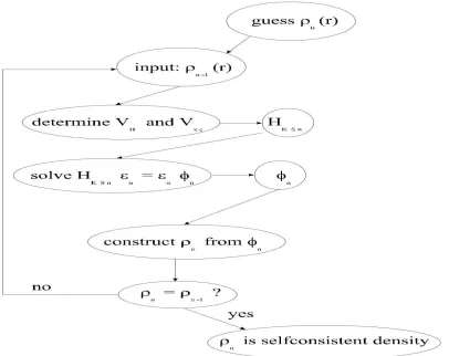
cannot be written down and solved before its solution is known. An iterative procedure is adopted to solve the

problem as shown in fig. 1. Some starting density ρ0 is guessed, and a hamiltonian HKS1 is constructed with it. The eigen value problem is solved, and results in a set of ϕ1 from which a density ρ1 can be derived. Most probably ρ0 will differ from ρ1. Now ρ1 is used to construct HKS2, which will yield a ρ2, etc. The procedure can be set up in such a way that this series will converge to a density ρf which generates a HKSf which yields as solution again ρf : this final

density is then consistent with the hamiltonian. To know the exchange-correlation functional we use approximations, one such approximation is called the Local Density Approximation (LDA)[6]. It means that the

exchange-correlation energy due to a particular density ρ( ) could be found by dividing the material in

1792 | P a g e

Figure 1: Flow chart for the n

th

iteration in the selfconsistent procedure to solve Kohn-Sham

equations

Each such volume contributes to the total exchange correlation energy by an amount equal to the exchange

correlation energy of an identical volume filled with a homogeneous electron gas, that has the same overall density

as the original material has in this volume. Another approximation is called the Generalized Gradient

Approximation (GGA)[7]. The exchange-correlation contribution of every infinitesimal volume not only dependent

on the local density in that volume, but also on the density in the neighbouring volumes.

Solving the Kohn – Sham equations

:

Solving in most methods means that we want to find the coefficients needed to express ϕm in a given basis set . If the functions of the basis set are very similar to ϕm, one needs only a few of them to accurately describe the

wave function, and hence P and the matrix size are small. Such a basis set is called efficient. But such a basis set can

never be very general: for some specific problems it will very quickly yield the solution, but for the majority of

1793 | P a g e

affordable, and limiting P would lead to approximate eigenfunctions that are not acceptable. These approximations carry too much properties from the basis function, and such a basis set is therefore called biased. The art of

theoretical condensed matter physics is to find a basis set that is a simultaneously efficient and unbiased.

III The pseudopotential Method

Two principal requirements for a basis set in which we want to expand the eigenstates of the solid state Hamiltonian

are : the basis set should be unbiased and efficient. A basis set that is certainly unbiased and simple is the plane wave basis set that can be used to express any eigenfunction of a periodic Hamiltonian[8] can be expressed

exactly in this basis set by means of an infinite set of coefficients.

In practice we cannot work with an infinite basis set, and will have to limit it. For plane waves, this can be easily

done by limiting the set to all K with K ≤ Kmax . This corresponds to a sphere with radius Kmax centered at the origin

of reciprocal space. All reciprocal lattice vectors that are inside this sphere are taken into the basis set.

Fig.2: Radial part of wave function (a) and radial probability distribution (b) of a 3s electron in Ca

(Y-axis has arbitrary units).

The number of plane waves is determined by the smallest length scales that are to be described in real space.

Consider the radial part of a 3s wave function in Ca (fig. 2). Near the nucleus, the wave function shows steep

behaviour. In order to describe the sharp part between 0 and the minimum at 0.1 A plane waves with a period as

small as roughly an order of magnitude less than this distance are needed (0.01 A or 10 m). This sets the order of

1794 | P a g e

matrices, which is way beyond the capability of even supercomputers. In order to overcome this problem we replace

the potential in these inner regions by a pseudopotential, that is designed to yield very smooth tails of wavefunctions

inside the atom hence only a few plane waves are needed. In the outer regions of the atoms, the pseudopotential

continuously evolves into the true potential, such that this region of the crystal behaves as if nothing happened. In

this way, it is possible to use an plane wave basis set. To judge whether a particular pseudopotential is good:criteria

is softness and transferability. A pseudopotential is called soft when few plane waves are needed. A specific class of

pseudopotentials is even called ultrasoft[9], because of the very small amount of plane waves it calls for. Also the

potential that can be used in whatever environment (molecule, cluster, solid, surface, insulator, metal) the

corresponding element can be. Such a pseudopotential is called transferable. Good pseudopotentials are those

potentials that are both (ultra)soft and transferable.

IV AUGMENTED PLANE WAVE (APW) METHOD

If you are interested in information that is inherently contained in the region near the nucleus (hyperfine fields for

instance, or core level excitations) then we will search for a basis set that uses other functions than plane waves, and

that does not require the introduction of a pseudopotential. Such a basis set is called the Augmented Plane Wave

(APW) basis set[10]. Close to the nuclei, the electrons behave quite as they were in a free atom, and they could be

described more efficiently by atomic like functions. Space is therefore divided now in two regions: around each atom a sphere with radius Rα is drawn (call it Sα). Such a sphere is often called a muffin tin sphere, the part of space occupied by the spheres is the muffin tin region. The remaining space outside the spheres is called the interstitial region (call it I). One augmented plane wave (APW) used in the expansion of is defined as

The APW basis set is k-dependent, as was the plane wave basis set. The are spherical harmonics. If an

eigenfunction would be discontinuous, its kinetic energy would not be well-defined. Such a situation can therefore

never happen, and we have to require that the plane wave outside the sphere matches the function inside the sphere

over the complete surface of the sphere

In order to describe an eigenstate ( ) accurately with APW’s, one has to set E equal to the eigenvalue (or band

energy) of that state. In practice, Kmax≈ 3.5 au−1 is needed for sufficient accuracy. This is less than the typical value

of 5.5 for plane waves and pseudopotentials. The calculation time (mainly determined by matrix diagonalization)

scales with the third power of the basis set size, which would suggest APW to be 10 times faster than

1795 | P a g e

with APW one diagonalization is needed for every eigenvalue. This makes the APW method inherently slow, much

slower than the pseudopotential method.

V LINEARIZED AUGMENTED PLANE WAVE METHOD (LAPW)

The problem with the APW method was that the uαℓ(r′, E) have to be constructed at the yet unknown eigenenergy E

of the searched eigenstate. If we calculate uαℓ at some energy E0,we could make a Taylor expansion to find it at energies not far away from it.

Substituting the first two terms of the expansion in the APW for a fixed E0 gives the definition of an LAPW[11]. But here the energy difference E0 - is unknown.

In order to determine both unknown parameters we will require that the function in the sphere matches the plane

wave both in value and in slope at the sphere boundary. This results in a 2 × 2 system from which both coefficients can be solved. we want to describe an eigenstate that has predominantly p-character (ℓ = 1) for atom α. This

means that in its expansion in LAPW’s, the are large. It is therefore advantageous to choose E0 near the

centre of the p-band. We can repeat this argument for every physically important ℓ (s-, p-, d- and f-states, i.e. up to ℓ

= 3) and for every atom. The final definition of an LAPW is then:

With the being fixed, the basis functions can be calculated once and for all.The same procedure as used for the

plane wave basis set can now be applied. One diagonalization will yield P different band energies for this . The accuracy of a plane wave basis set was determined by Kmax . However, a better quantity to judge the accuracy here is

1796 | P a g e

the closest point a plane wave can come to a nucleus moves farther away from the nucleus. The part of the wave

function that need not to be described with plane waves any more, in general will have displayed the steepest

behaviour, steeper than anywhere else in the interstitial region. Less plane waves are needed to describe the

remaining, smoother parts of the wave function. Kmax can be reduced, and a good rule of thumb is that the product

RαminKmax should remain constant in order to have comparable accuracy. Compared to a plane wave basis set, the

LAPW basis set can be much smaller. The calculation time (mainlydetermined by matrix diagonalization) scales

with the third power of the basis set size, which makes LAPW in this respect about 2 to 3 times faster than plane

waves.

VI LINEARIZED AUGMENTED PLANE WAVE METHOD WITH LOCAL ORBITALS

(LAPW+ LO)

It often happens that states with the same ℓ but a different principal quantum number n are both valence states . Such

low-lying valence states are called semi-core states. These states are solved by adding another type of basis function

to the LAPW basis set, called a local orbital (LO)[12]. A local orbital is defined for a particular ℓ and m, and for a

particular atom α. A local orbital is zero in the interstitial region and in the muffin tin spheres of other atoms, hence its name local orbital. Local orbitals are not connected to plane waves in the interstitial region, they have hence no

and dependence. Adding local orbitals increases the LAPW basis set size. If for each atom local orbitals for p-

and d-states are added, the basis set increases with 3+5=8 functions per atom3 in the unit cell. This number is rather

small compared to typical LAPW basis set sizes of a few hundred functions. The slightly increased computational

time is a small price to be paid for the much better accuracy that local orbitals offer, and therefore they are always

used.

VII AUGMENTED PLANE WAVE (APW) METHOD WITH LOCAL ORBITALS (APW+ LO) :

In the APW+lo method that will be described now, the basis set will be energy independent and still have the same

size as in the APW method. In this sense, APW+lo combines the good features of APW and LAPW+LO. The

APW+lo basis set contains two kinds of functions. The first kind are APW’s, with a set of fixed energies .

1797 | P a g e

both the APW and the local orbital are continuous at the sphere boundary, but for both their first derivative is

discontinuous. It is advantageous to treat those states having high with APW+lo, and keep using LAPW for

all other states. Using APW+lo[13] for a state means that per atom 2ℓ + 1 local orbitals are added to the basis set.

This makes an APW+lo basis set for the same Rαmin Kmax considerably larger than the LAPW basis set. This is

compensated by the fact that a lower Rαmin Kmax is needed for accurate results, but nevertheless, it is better to use

these extra basis functions only there where they are useful. Such an approach leads to a mixed LAPW/APW+lo

basis set: for all atoms α and values of ℓ.

VIII PROJECTOR AUGMENTED WAVE METHOD (PAW):

A third major way to obtain basis sets that are simultaneously unbiased and efficient is the Projector Augmented

Wave method (PAW). The goal of PAW[14] is to express the single particle all-electron Kohn-Sham wave functions

). In PAW write the all-electron wave function as a sum of a few other functions, each of which can be

expressed in a natural way in a basis.

The first term at the right-hand side of above equation is the pseudo wave function ψn( ). This function is identical

to the all-electron single-particle Kohn-Sham wave function except inside the augmentation spheres. The

atom-centered augmentation spheres play a role that is similar to the muffin tin spheres in the APW-based methods[15]. Inside the augmentation spheres, the pseudo wave function will be much smoother than the all electron wave

function, which is similar to what happens in the pseudopotential method. These transformation operators are such

that they transform the pseudo wave function inside sphere a into the all-electron wave function. Selecting appropriate projector functions for each element of the periodic table is a kind of art, and can have considerable

effect on the speed and accuracy of the DFT calculation. PAW-based DFT codes typically provide one or more choices of projector functions[16] for every element of the periodic table. The all-electron single-particle

Kohn-Sham wave function (steep near the nuclei and smooth elsewhere) can be written as the sum of (1) a pseudo wave

function that is smooth everwhere, to which is added (2) a steep function that is defined only within each

augmentation sphere, and from which is subtracted (3) the smooth part, only within the spheres. (1) can be

conveniently represented in a plane wave basis, (2) is already represented in the basis of partial waves, and (3) is

1798 | P a g e

IX CONCLUSION

Attempts to extend the applicability of ab initio DFT methods to even larger systems have been greatly assisted by

the improved performance of commodity clusters. The challenge is now to improve the performance of calculations

involving computationally more demanding approaches such as hybrid functionals. Finally, with applications of the

methods spreading to ever new areas, new “tools” for the calculation of materials properties, spectra, processes will

be required. This exceeds by far the potential of a single group of developers. Here we hope that the development of

the different simulation packages add to development of ab initio methods.

REFERENCES

1. Kohn, W.; Sham, L. J. Phys Rev A 1964, 140, 1133.

2. Parr, R. G.; Yang, W. Density Functional Theory of Atoms and Molecules; Oxford University Press: Oxford, UK,

1989.

3. Perdew, J. P; Schmidt, K. In Density Functional Theory and its Applications to Materials,; Van Doren, V.; van

Alsenoy, C.; Geerlings, P., Eds.; AIP: Melville, NY, 2001.

4. Perdew, J. P. ; Kurth, S. In A Primer in Density Functional Theory; Fiolhais, C.; Nogueira, F.; Marques, M., Eds.;

Lecture Notes in Physics, vol. 620; Springer: Berlin, 2003.

5. Perdew, J. P.; Zunger, A. Phys Rev B 1981, 23, 5048.

6. Becke, A. D. Phys Rev A 1988, 38, 3098.

7. Becke, A. D. J Chem Phys 1993, 98, 1372.

8. Perdew, J. P. Phys Rev B 1986, 33, 8822.

9. van Voorhis, T.; Scuseria, G. E. J Chem Phys 1998, 109, 400.

10. Boese, A. D.; Handy, N. C. J Chem Phys 2002, 116, 9559.

11. Becke, A. D. J Chem Phys 1998, 109, 2092.

12. Tao, J. J Chem Phys 2001, 115, 3519.

13. (a) Tao, J. J Chem Phys 2002, 116, 2335; (b) Tao, J. J Chem Phys 2002, 116, 10557 (E).

14. Kurth, S.; Perdew, J. P., Blaha, P. Inter J Quantum Chem 1999, 75, 889.

15. Stevens, P. J.; Devlin, F. J.; Chablowski, C. F.; Frisch, M. J. J Phys Chem 1994, 80, 11 623.