The Parallel Asynchronous Differential Evolution Method as a Tool to Analyze Synchrotron Scattering Experimental Data from Vesicular Systems

(1)

The

Parallel

Asynchronous

Differential

Evolution

Method

as a Tool to Analyze Synchrotron Scattering Experimental Data

from Vesicular Systems

Evgeniya Zhabitskaya1,2,a_{, Elena Zemlyanaya}1,2_{, Mikhail Kiselev}1,2_{, and Andrey Gruzinov}3

1_{Joint Institute for Nuclear Research, Joliot-Curie 6, 141980 Dubna, Russia} 2_{Dubna State University, University str. 19, 141980 Dubna, Russia}

3_{National Research Center «Kurchatov Institute», Moscow, Russia}

Abstract.

In this work we use an Asynchronous Differential Evolution (ADE) method to estimate parameters of the Separated Form Factor (SFF) model which is used to investigate a struc-ture of drug delivery Phospholipid Transport Nano System (PTNS) unilamellar vesicles by experimental small angle synchrotron X-ray scattering spectra (SAXS). We compare the efficiency of different optimizing procedures (OP) for the search for the SFF-model parameters. It is shown that the probability to find the global solution of this problem by ADE-methods is significantly higher than that by either Nelder-Mead method or a Quasi-Newton method with Davidon-Fletcher-Powell formula. The parallel realization of ADE accelerates the calculations significantly. The speed-up obtained by the parallel realization of ADE and results of the model are presented.

1 Introduction

Diﬀerential Evolution (DE) [1] is an eﬃcient algorithm to solve global optimization problems. Recent

progress in the development of DE is summarized in the book [2] and in the review article [3]. The

Asynchronous Diﬀerential Evolution (ADE) method [4] incorporates classical DE mutation, crossover

and selection operations into a parallel steady-state strategy. It is well suited for parallel optimization. ADE with independent restart [5] automatically adapts the population size to the complexity of the problem. ADE with a restart and adaptive correlation matrix [6] (ADE-ACM) automatically adapts to the landscape of the optimized objective function.

In [7, 8] the method of separated form factors (SFF) is adapted for the analysis of experimental data on small angle synchrotron X-ray scattering (SAXS) to polydispersed population of dimiros-toilphosphatidilholin (DMPC) unilamellar vesicles (ULVs), placed in an aqueous solution of sucrose. In this work we employ this method for the analysis of SAXS spectra from the drug delivery Phospho-lipid Transport Nano System (PTNS) [9]. Parameters of the SFF model are estimated with the help of ADE method. The calculations have been also made using other popular minimization algorithms in

order to compare the eﬃciency of diﬀerent approaches.

(2)

2 Materials and methods, mathematical model and numerical algorithm

The PTNS samples for the SAXS measurements were prepared via dilution of lyophilized PTNS in such a way that to have 20%, 25%, 30% and 35% of maltose concentration in water. The mea-surements were performed at room temperature at the DICSI station of the Kurchatov Synchrotron

Radiation Source in Moscow, Russia. The scattering intensitiesIexp.₍_q_{) of photons from liophylized}

PTNS solutions in water are measured as a function of the scattering vectorq=4πsinθ₂/λ, whereθ

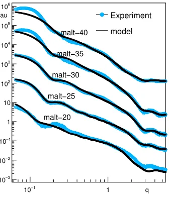
is the photon scattering angle. Experimental data are shown in Fig. 1 by light circles. The plot is the

subtraction of the PTNS intensity and the corresponding buﬀer intensity from maltose solution.

In the data analysis we employ an approach based on the SFF method [7]. In this framework the macroscopic cross-section of the polydispersed vesicular population is of the form

dΣ

dΩ(q)=n I0FˆsFˆbSF, (1)

whereI0is the intensity of the incident beam,nis the number of vesicles in unit volume,SF(q;R,n)

is the structural factor1_{. Considering the polydispersity of the vesicular radii like in [7, 8]}2_{and taking}

into account the ﬂuctuations of the parameters of the internal structure of the bilayer3_{, the form factor}

of the population of spherical vesicles ˆFsand the form-factor of the bilayer ˆFbare:

ˆ

Fs(q;R,m) =

Rmax

Rmin

Fs(q,R)G(R,R,m)dR Rmax

Rmin

G(R,R,m)dR, (2)

ˆ

Fb(q,Θb,kﬂ) =

K

−K

Fb(q,Θb(Θb,kﬂ, ξ))f(ξ)dξ

K

−K

f(ξ)dξ. (3)

The form factor of the spherical surface with radiusRis Fs(q;R) = (4πR2sin(qR)/qR)2. The form

factor of the symmetric lipid bilayer isFb(q,Θb) =( ₊d/2

−d/2 ρc(x) cos(qx)dx)

2_{. The contrast function}

ρ(x;Θb) is described by the parameters of the internal structure:Θb={d,D,L, ρH}.

In view of the incoherent background (IB) and spectrometer resolution, the macroscopic cross section takes the form:

I(q)= dΣ

dΩ(q)+

1

2Δ

2d 2dΣ

dΩ(q)

dq2 +IB, (4)

whereIBis the parameter of incoherent background,Δ2=3.6·10−7cm2is the second momentum of

the spectrometer resolution function.

The ﬁt of the experimental data was carried out by minimizing the objective function describing the discrepancy between the theoretical and experimental values of the intensity

f(Θ)=

N

j=1

I(qj,Θ)−Iexp(qj) σ2₍_q

j)

2

, Θ∗₌_{Arg min}

Θi

f(Θ), (5)

1_{The structural factor considers inter-vesicular interaction. In the Debye approximation}_S₍_q_;_R_,_n₎₌ ₁₋8Vν ν

sin(2qR) 2qR

, whereV_ν=4πR3_/_{3 is the vesicle volume,}_ν₌₁_/_n_{is the volume of the solvent per one vesicle.}

2_{The polydispersity of vesicular population is described by the asymmetric Schulz distribution} _G₍_R_,_R_,_m₎ ₌

Rm_/_m_!(_m₊₁_/_R₎m+1_exp[₋₍_m₊₁₎_R_/_R_]_,_where_R_{is the average radius of the vesicles,}_m_{is the polydispersity}

parame-ter. In the calculations belowRmin=1 nm,Rmax=8.1 nm.

3_{In the calculations presented below, it is assumed that the di}_ﬀ_{erence in the values of parameters of the internal structure}

is due to the ﬂuctuation of the thickness of the membrane. Then the components ofΘbin the integral in Eq. (3) are, respec-tively:d=d(1+kﬂξ),D=D

1+_Ddkﬂξ

,L=L1−d_Lkﬂξ

(3)

1

−

10 1 q au

3

− 10

2

− 10

1

− 10

1 10

2

10

3

10

4

10

5

10

6

10

Experiment

malt−20 malt−25

malt−30 malt−35

malt−40 model

d1

r0

rL

d

D

rH

L

rM

h s

Figure 1. SAXS spectra from the PTNS vesicles in 20–40%(w/w) maltose solution in water. Circles — ex-periment, solid line — theory.

Figure 2. Structure of a phospholipid unilamellar vesicle with radius R and the “two-step” scattering length density (contrast function) ρ(x;Θb) across bi-layer; Θb = {d,D,L, ρH}; parametersρ0, ρM, ρL are ﬁxed.

Table 1.The boundaries of the search area and the coordinates of the minima for the two step SFF model. Accuracy in the table is equal to the last signiﬁcant digit. The number of data points isN=1000.

Model R,

nm m

l, nm

s, nm

h,

nm kﬂ

ρH,

×1010

cm−1

nI0,

×1018

cm−3

IB,

×10−3

a.u. Vν

ν f

∗

min(Θ∗) N

Θmin

i 8.0 5.0 0.01 0.0 0.8 10−5 10.1 10−4 −100 0.02

Θmax

i 25.0 30.0 1.50 3.50 1.0 0.2 14.0 10−1 100 0.08

PTNS-20 21.9 12.9 0.322 1.33 0.900 0.2 12.7 0.0024 2.34 0.07 1.008

PTNS-25 17.1 20.3 0.100 1.14 1.00 0.147 11.4 0.0172 3.76 0.08 0.318

PTNS-30 14.3 16.9 0.403 1.07 0.820 0.106 11.4 0.0264 2.15 0.02 0.531

PTNS-35 13.1 14.1 0.000 1.09 0.819 0.095 11.3 0.0421 1.99 0.02 1.70

PTNS-40 10.6 9.34 0.184 1.71 0.977 0.2 12.6 0.0267 1.27 0.02 1.80

whereNis the number of experimental points,σis the error estimations, the set of the varied

param-eters isΘ ={R,m,l,s,h,kﬂ, ρH,nxI0,IB,Vν/ν}.

(4)

3 Comparison of the effectiveness of ADE, ADE-ACM, Nelder-Mead

simplex and quasi-Newtonian with Davidon-Fletcher-Powell formula

optimization methods

To ﬁnd the minimum (5), diﬀerent methods of optimization have been used: in addition to the

vari-ous strategies of ADE [4, 5] and ADE with Adaptive Correlation Matrix (ADE-ACM) [6] methods, there are the Nelder–Mead simplex method [10] and the quasi-Newtonian method with Davidon– Fletcher–Powell formula [11, 12]. As part of the ROOT-Minuit program [13], these methods are called SIMPLEX and MIGRAD, respectively.

The permissible search area for all the optimization procedures (OPs) has been set as: Θj ∈

[Θmin

j ,Θmaxj ]. TheΘminj andΘmaxj values are presented in 2ndand 3rdlines of the Table 1. The points

for the initial approximation are uniformly distributed in this area for all methods tested. The

ADE-method is used in two ways. (i) ADE rand/rand/1/bin strategy: in this case, the values have

been set for the scaling factor as F = 0.9 and for crossoverCr = 0.9. (ii) ADE-ACM strategies

rand/rand/1/acmandlinworst/current-to-pbest/1/acm. In both cases, the initial population isNinit

p =32, the restart criteria isΔxk=10−12, the minimum required accuracy of localization (exit criteria)

isΔf =10−2_{(see [5] for details). In the settings of SIMPLEX and MIGRAD methods the maximum}

number of the function evaluations allowed were increased in comparison with the default settings4_.

The calculations were repeated by each methodnt=100 times.

The minimal values of the function f_min∗ (Θ∗) for each model have been found at the pointsΘ∗,

the coordinates of which are given in lines 4 – 8 of Table 1. Note that some of the SFF parameters are in signiﬁcant correlation in the vicinity of the minimum. Moreover, each problem has several local minima. This complicates the process of minimization.

A comparison of the eﬀectiveness of ADE, ADE-ACM, SIMPLEX and MIGRAD methods is

shown in Fig. 3. On the horizontal axis the diﬀerence between the best value founded by ith

opti-mizing procedure f_i∗(Θ) and the minimal obtained value f_min∗ (Θ∗) is laid. On the vertical axis we

give the percentage of attempts with the same or better result received by each of the methods used. Table 2 shows the summarized results obtained by each method. The probability of ﬁnding the so-lution by SIMPLEX method was found to be 1 – 2% (see col. 3 of Table 2). Most often, this method diagnoses convergence at points far from the global minimum and stops further calculations. The

probability of ﬁnding the solution5_{of the problem by MIGRAD is close to 40% .}

At the same time, all the tested strategies of ADE converged to the global minimum with

a probability of more than 70%, and the most successful (DE/rand/rand/1/acm) — with a

prob-ability of more than 90%. Note that this probability could be further enhanced by increasing

the maximum number of function evaluations allowed. The use of the adaptive crossover can in-crease the probability of ﬁnding the global minimum signiﬁcantly. The use of “fast track” strategy

DE/linworst/current-to-pbest/1/acmreduces the average number of function evaluations approxi-mately three times, but this strategy has a larger probability of ending calculations in one of the local minima.

Thus, in dealing with this problem, ADE are to be preferred to the classical ones for several reasons. First, ADE and ADE-ACM are robust global minimum search methods. They end the calcu-lations with a larger probability at the minimum of the problem, while the search using SIMPLEX and

MIGRAD ended at the minimum with a chance of 1±1% and 43±7%, respectively. The probability

of ﬁnding the global minimum by ADE-R depending on the chosen strategy varied fromp=73±5%

4_{MaxFunctionsCalls}₌_{300 000, which is enough for these programs to ﬁnish computations before the MaxFunctionsCalls}

is reached.

5_{Assuming that the minimum has been founded if}_δΔ2₌_f∗

i(Θ)−fmin∗ (Θ∗)

2

(5)

Table 2.Eﬃciency of the optimization procedures (OP), based on diﬀerent optimization methods.†Ninit

p =32.

The percentage of successful (δΔ = f_i∗(Θ)−fmin∗ (Θ∗)≤1) attempts, average number of function

evaluationsNFEand median number of function evaluations MedNFEfor each method.

Method MIGRAD SIMPLEX ADE

† _ADE-ACM†

rand/rand/1/bin rand/rand/1/acm linworst/curtopbest/1/acm

δΔ2_≤₁ _43% _1% _73% _93% _76%

NFE 3650±140 3500±170 29000±3000 89000±7300 20600±900

MedNFE 3120±270 3650±370 16760±1500 50000±34000 18500±1100

f−f

5

−

10 10−410−310−210−1 1 10 102 103 104

n

0 20 40 60 80

100 DE/rand/rand/1/bin, Np=32 DE/rand/rand/1/acm, Np=32 DE/linworst/current−to−pbest/1/acm, Np=32 SIMPLEX

MIGRAD

Nproc

1 10 102

speed−up

1 10

2

10 speed−up T

speed−up tau

Figure 3. Comparison of the eﬀectiveness of various OP solving SFF for PTNS-30 problem. Horizontal axis: the diﬀerence between the best value, found byith_OP _f∗

i(Θ)

and the global minimum f_min∗ (Θ∗); vertical axis: percent-age of attempts with same or better result, received by the methods. DE−rrbmeansDE/rand/rand/1/binmethod;

DE−rra means DE/rand/rand/1/acm; DE−lwa means

DE/linworst/current-to-pbest/1/acm; SIM. means SIM-PLEX; MIG. means MIGRAD.

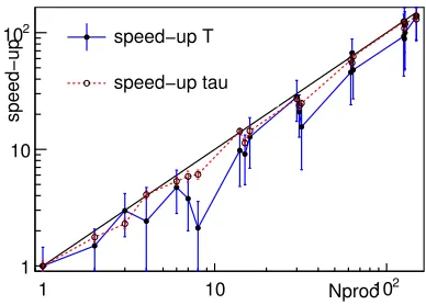
Figure 4. Acceleration of parallel computing (speed-up) depending on the number of calcu-lating processors Nproc used. Solid line — re-sultant acceleration — decrease in mean whole calculation timeT; dashed line — acceleration for mean time of one calculation of the objective functionτ.

(forDE/rand/rand/1/bin) top=93±3% (forDE/rand/rand/acm). On the other hand, if necessary, to ﬁnd the secondary minima, preliminary ADE-produced results during calculations can be used.

As a direct (without the use of derivatives) method, ADE continues calculations and ﬁnds solutions in situations where quasi-Newton Davidon-Fletcher-Powell’s method diagnoses inability of further searches, and the simplex method completes the calculations and does not come close to the minimum.

4 ADE speed-up for parallel computation

The average number of function evaluationsNFEfor ADE and ADE-ACM larger than that for

clas-sical methods. However, the use of parallel computations signiﬁcantly reduces the actual time-out of

the ADE methods [14] (see Fig. 4). The eﬀectiveness of MPI-based6 parallel implementation of the

ADE algorithm have been tested on the multi-processor cluster CICC (LIT, JINR Dubna).

(6)

The calculations of the SFF model for PTNS-30 with two-step density approximation have been

repeatedly run for diﬀerent numbers of computational nodes:Nproc∈[2,150].

Since the ADE algorithm is non-deterministic, the number of function evaluations required to achieve a certain accuracy is varying and its average value is slightly increasing with the increase of the number of parallel processors used.

Fig. 4 shows nearly linear speed-up up toNproc=150 nodes involved in parallel computing. The

solid line shows the resultant acceleration. The dotted line shows speed-up per one calculation of the

objective function. This acceleration is associated with maxNFEstopping criteria.

5 Conclusions

The parameters of a polydispersed population of unilamellar vesicles PTNS, including the internal structure of the lipid bilayer of vesicles membrane have been estimated by the ADE-method. The optimization procedures implemented on the basis of ADE and ADE-ACM methods were compared with the OPs, implemented on the basis of commonly used methods SIMPLEX and MIGRAD. It is shown that the probability of obtaining a correct solution to the optimization problem by the ADE methods considerably exceeds the probabilities for the SIMPLEX and MIGRAD methods. The speed up in parallel MPI-based calculations has been estimated. Thus, it is shown that ADE is well suited for the parallel computation of the vesicular systems parameter estimations.

References

[1] Price K. V. and Storn, R.V., J. of Global Optimization11, 341–359 (1997)

[2] Price K.V., Storn R.M., Lampinen J.ADiﬀerential Evolution: A Practical Approach to Global Optimiza-tion. Springer (2005)

[3] Das S., Suganthan P.N., IEEE Trans. Evol. Comput.15, 4–31 (2011)

[4] Zhabitskaya E.I. and Zhabitsky M.V., Lecture Notes in Computer Science7125, 328–333 (2012) [5] Zhabitskaya E. and Zhabitsky M., Lecture Notes in Computer Science8236, 555–561 (2013)

[6] Zhabitskaya E.I. and Zhabitsky M.V.,Proceeding of the 15th Annual Conference on Genetic and Evolu-tionary Computation, (USA, New York, 2013) 455–462

[7] Kiselev M.A., Zemlianaia E.V., Zhabitskaia E.I. and Aksenov V.L., Crystallography Reports60, 143–147 (2015)

[8] Zhabitskaia E.I., Zemlianaia E.V. and Kiselev M.A., Vestnik Rossijskogo universiteta druzhby narodov, seriia: Matematika. Informatika. Fizika2, 253–259 (2014)

[9] Kiselev M.A., Zemlyanaya E.V., Ipatova O.M., Gruzinov A.Yu., Ermakova E.V., Zabelin A.V., Zhabitskaya E.I., Druzhilovskaya O.S. and Aksenov V.L., Journal of Pharmaceutical and Biomedical Analysis114, 288–291 (2015)

[10] Nelder J.A. and Mead R., Computer J.7, 308–313 (1965)

[11] Davidon W.C., A.E.C. Res. and Develop. Report ANL-5990(Argonne National Laboratory. Argonne; Illinois, 1959) p. 21

[12] Fletcher R. and Powell M.J.D., Comput. J.6, 163–168 (1963)