DOI: 10.1534/genetics.105.048074
The Power of Single-Nucleotide Polymorphisms for Large-Scale
Parentage Inference
Eric C. Anderson
1and John Carlos Garza
Fisheries Ecology Division, Southwest Fisheries Science Center, Santa Cruz, California 95060
Manuscript received July 11, 2005 Accepted for publication December 8, 2005
ABSTRACT
Likelihood-based parentage inference depends on the distribution of a likelihood-ratio statistic, which, in most cases of interest, cannot be exactly determined, but only approximated by Monte Carlo simulation. We provide importance-sampling algorithms for efficiently approximating very small tail probabilities in the distribution of the likelihood-ratio statistic. These importance-sampling methods allow the estimation of small false-positive rates and hence permit likelihood-based inference of parentage in large studies involving a great number of potential parents and many potential offspring. We investigate the performance of these importance-sampling algorithms in the context of parentage inference using single-nucleotide polymor-phism (SNP) data and find that they may accelerate the computation of tail probabilities.1 millionfold. We subsequently use the importance-sampling algorithms to calculate the power available with SNPs for large-scale parentage studies, paying particular attention to the effect of genotyping errors and the occurrence of related individuals among the members of the putative mother–father–offspring trios. These simulations show that 60–100 SNPs may allow accurate pedigree reconstruction, even in situations involving thousands of potential mothers, fathers, and offspring. In addition, we compare the power of exclusion-based parent-age inference to that of the likelihood-based method. Likelihood-based inference is much more powerful under many conditions; exclusion-based inference would require 40% more SNP loci to achieve the same accuracy as the likelihood-based approach in one common scenario. Our results demonstrate that SNPs are a powerful tool for parentage inference in large managed and/or natural populations.
G
ENETIC markers have been used to infer parent-age in applications across a range of fields from anthropology and ecology to forensics and law. Today the molecular markers of choice for parentage in-ference are highly polymorphic, repetitive loci such as the short tandem repeat loci commonly employed in human parentage testing (Hammond et al. 1994) andthe microsatellites used in the field of molecular ecol-ogy (Quelleret al.1993). In contrast, single-nucleotide
polymorphisms (SNPs) have not been widely employed for parentage inference and other forms of relation-ship estimation, because, possessing only two alleles, each SNP has lower resolving power per locus than most microsatellites (Glaubitzet al. 2003). However,
SNPs have a number of features making them appro-priate for large-scale genetic studies: they are abundant in most genomes surveyed (Brumfield et al. 2003);
genotyping error rates are low (Ranade et al. 2001);
scoring SNP genotypes requires minimal human inter-action, making them amenable to high-throughput, low-cost genotyping; and SNP genotypes are easily stan-dardized across laboratories. Indeed, because of these
attractive features, SNPs have recently been employed for individual identification and paternity inference in large herds of cattle (Heatonet al. 2002; Werneret al.
2004) and for human forensic purposes (Lee et al.
2005).
Recently, several articles have reported specifically on the utility of SNPs for parentage inference, either for inferring parent–offspring pairs (Glaubitzet al.2003)
or for inferring paternity given an offspring, a known mother, and a candidate father (Krawczak1999; Gill
2001). All of these studies measured the power for par-entage inference in terms of the probability of exclusion (PE) (Chakraborty et al.1988). The PE is an
appro-priate measure of power if the actual inference is done on the basis of exclusion—that is, if candidate parents are to be eliminated from consideration because of Mendelian incompatibilities with the candidate off-spring. Although the method of exclusion is widely used, it has several important limitations. First, it uses only a portion of the information available in the data, and second, the method of exclusion is not easily ad-justed to account for genotyping error. A more powerful method of parentage inference was introduced by Thompson(1976). This method, based on a
likelihood-ratio statistic, is easily extended to allow for the pos-sibility of genotyping error and has been implemented
1Corresponding author:Fisheries Ecology Division, Southwest Fisheries
Science Center, Santa Cruz Laboratory, 110 Shaffer Rd., Santa Cruz, CA 95060. E-mail: [email protected]
in various categorical assignment methods and com-puter programs (Meagherand Thompson1986; S
an-Cristobaland Chevalet1997; Marshallet al.1998;
Gerberet al.2000; Duchesneet al.2002). For a recent
review of the different approaches and methods avail-able for inference of parentage, see Jonesand Ardren
(2003).
The level of confidence in inference from likelihood-based methods depends on the distribution ofL, the log-likelihood ratio statistic, given the allele frequencies and other details of the sampling design. In general, the distribution ofLis not analytically tractable, so its dis-tribution is approximated by Monte Carlo simulation; however, none of the currently available Monte Carlo methods are suitable for estimating expected error rates in parentage studies involving large numbers of poten-tial parents and offspring. This is a consequence of the large number of possible trios (putative mother, puta-tive father, and putaputa-tive offspring) that must be in-vestigated in large studies. There can potentially be billions of trios in such a study, and therefore per-trio false-positive rates on the order of one in 1 billion are relevant. Standard, ‘‘naive’’ Monte Carlo estimates of such small probabilities are inaccurate and computa-tionally impractical.
In this article, we develop importance-sampling methods (Hammersley and Handscomb 1964) that
allow very small tail probabilities in the distribution ofL
to be estimated accurately and rapidly. These methods make likelihood-based inference in large-scale studies practical. We then assess the power of SNPs for likelihood-based parentage inference from trios. The results are presented in terms of trio false-positive and per-trio false-negative rates, from which it is straightforward to estimate expected studywide error rates (i.e., the ex-pected absolute number of misassignments of offspring to parents). In addition, we incorporate the effects of genotyping error in the method by accounting for this error in both the likelihood-ratio and the Monte Carlo simulations, and we consider a wide range of possible nonparental relationships that can occur among three individuals. Our main interests are in situations where neither the true mother nor the true father of the child is known. However, cases where the true mother (or father) is known are handled easily within the same framework, and results are presented for such cases. Ultimately we show that with only a moderate number—
60–100—of SNPs, enough power is achieved to accu-rately infer parentage in quite large populations.
In methods we describe likelihood inference of
parentage and the importance-sampling methods. In
resultswe provide calculations of per-trio error rates
for a variety of different trio relationship categories, and we show that likelihood-based methods are more power-ful than exclusion-based methods. We then show how such calculations can be used to provide expected study-wide error rates, using a scenario from a hypothetical
salmon population. In the discussion, we address
several issues relevant to large-scale parentage studies with SNPs. Most importantly we point out that, for many scenarios, genetic linkageper seis not a great concern, although linkage disequilibrium between SNP markers can reduce power for parentage inference.
METHODS
The use of likelihood to infer relationships between in-dividuals was proposed by Edwards(1967). Thompson
(1976) developed likelihood-based methods for recon-structing human pedigrees by testing for parental rela-tionships. While Thompson(1976) reported on methods
for simultaneously inferring the parentage of large sib-ships, we focus on the inference of parentage in what Thompson refers to as ‘‘Q-triplets’’—trios of individuals consisting of a putative offspring, a putative mother, and a putative father. We denote these three individuals by y, m, and f, respectively. Ourmethodssection is organized as
follows. First, we present some notation for SNP markers and briefly review likelihood inference of parentage. Then, we show how false-positive and false-negative rates can be computed. And finally, we present an efficient Monte Carlo method for estimating probabilities of in-correct parentage assignment.
We assume that the genetic data consist of L SNP markers. There are typically only two states (alleles) that each SNP locus takes in a population. For example, at one locus the two alleles may be A and G; at a different locus the two alleles may be C and A, and so forth. Instead of using the letter names of the DNA bases at each locus, we use 0 to denote the minor allele—the one at lowest frequency in the population—and 1 to denote the allele at higher frequency. We letqdenote the fre-quency of the minor allele andp¼1qthe frequency of the other allele. Since there are only two alleles, there are only three diploid genotypes possible at each locus. We name these genotypes according to the number of 1 alleles that they contain. Hence a genotype of 0 is ho-mozygous for the 0 allele, a genotype of 1 is a hetero-zygote, and a genotype of 2 is homozygous for the 1 allele. The frequencies of these genotypes in the pop-ulation, assuming Hardy–Weinberg equilibrium, areq2,
2pq, andp2, respectively. Throughout most of this article,
we assume that the SNP markers are unlinked and are not in linkage disequilibrium (LD), but we briefly consider the effects of linkage in thediscussion.
Parent–pair likelihood inference:For a single trio of individuals, inferring whether m and f are both parents of y, an event that we denote byQ, or whether m, f, and y are three entirely unrelated individuals (U) is princi-pally done using the log-likelihood-ratio statistic:
L¼logPðGm;Gf;GyjQÞ
PðGm;Gf;GyjUÞ
P(Gm, Gf, Gy j Q) is the probability of the observed
genotypes of m, f, and y atLloci under the assumption that m and f are the parents of y.P(Gm,Gf,Gyj U) is
the probability of the observed genotypes under the assumption that m, f, and y are mutually unrelated individuals.
The above formulation of Thompson(1976) does not
account for genotyping error, which can be problem-atic. For example, a single genotyping error among a true parental trio could lead toP(Gm,Gf,GyjQ) being
zero, which would make L ¼ ‘, and one would wrongly reject the possibility that m and f were the parents of y. If independent estimates of the genotyping rates are known (or can be assumed), the analysis can be done conditional on those known (assumed) genotyp-ing error rates. We assume that genotypgenotyp-ing errors occur at a rate ofm‘per gene copy, and that they are inde-pendent between gene copies at a locus and between loci. This is a two-allele case of the error model con-sidered by SanCristobal and Chevalet (1997).
Be-cause there are only two allelic types, the genotyping error model can be made simple and realistic—a geno-typing error means that a 0 allele is observed as a 1 allele or that a 1 allele is observed as a 0 allele—without in-curring a large computational burden as with markers having multiple alleles (Sieberts et al. 2002). It is
possible that genotyping errors at the two gene copies at a locus would not occur independently of one another. In such a case the error model would have to be altered, which would not be difficult.
Assuming a genotyping error ratem‘. 0 at the‘th locus, the calculation of L is much like that in (1), except thatP(Gm,Gf,GyjQ) andP(Gm,Gf,GyjU) are
replaced byP(Gm,Gf,GyjQ,m) andP(Gm,Gf,GyjU,m),
respectively, the latter two being probabilities computed conditional on the locus-specific genotyping error rates m¼(m1,. . .;mL). Calculation ofP(Gm,Gf,GyjQ,m) and P(Gm,Gf,GyjU,m) is straightforward. Details appear in
theappendix.
In parentage inference, as typically pursued, if the statisticLis greater than some threshold value,Lc, then the trio is declared to be of type Q. If the trios being tested are all of either typeQor typeU, then rejecting hypothesis U is equivalent to accepting hypothesis Q, and parentage inference of this sort is formally a hypo-thesis test. If the genotyping error rate is known exactly, then by the Neyman–Pearson lemma (Neyman and
Pearson1933), a test based onLis the most powerful
test available (as noted by SanCristobaland Chevalet
1997). In other words, among all possible parentage tests, a test using the statistic in (1) will have the smallest type II error rate for any chosen type I error rate. The Neyman–Pearson lemma provides a theoretical justifi-cation for what has been noted by previous authors (Marshallet al.1998) and is demonstrated later in this
article—that likelihood-based methods can be more powerful than those based on parental exclusion.
If the trios being tested have some relationship other thanQorU, however, then such an analysis is not formally a hypothesis test, and the Neyman–Pearson lemma no longer applies. This means that without knowing the pattern of relatedness of the members of the trio—which is typically unknown—it is not possible to design a most powerful test for parentage. Nonetheless, the test statistic
L, with the likelihood ofUin the denominator, is still a reasonable choice of test statistic, even when the true relationship of the trio may be something other thanQor
U(Meagherand Thompson1986).
We express the power for trio-based parentage as-signment in terms of false-positive and false-negative error rates. These are analogs of type I and type II errors in hypothesis testing. A false-positive error occurs when we declare a trio to be of typeQwhen, in fact, it is not. A false-negative error occurs when we declare a trio tonot
be of typeQwhen, in fact, it is. The probabilityaof a false positive depends on the allele frequencies q ¼
(q1,. . .;q‘), the genotyping error rates m, the true relationship,T 6¼Q, of the individuals within the trio, and the chosen value ofLc. It is the probability that a trio
of type T yields L . Lc, which can be written as the
expected value
aðq;m;T;LcÞ
¼ET;m I logPðGm;Gf;GyjQ;mÞ
PðGm;Gf;GyjU;mÞ
.Lc
; ð2Þ
whereI fx.Lcgis the indicator function that takes the
value 1 ifx.Lcand 0 otherwise, and the subscript ‘‘T,
m’’ signifies that the expectation over all values of (Gm, Gf,Gy) is taken conditional on the trio being of typeT
and the genotyping error rates of the loci beingm. The probability of a false-negative error is the probability that a trio of typeQyieldsL,Lc, which is denoted by
bðq;m;LcÞ ¼EQ;m I log
PðGm;Gf;GyjQ;mÞ
PðGm;Gf;GyjU;mÞ
,Lc
:
ð3Þ
The quantitiesaandbareper-trioerror rates.b(q,m,
Lc), when multiplied by the number of parental trios
compared in a study, gives the expected number of false negatives in the whole study. Likewise a(q, m, T, Lc)
multiplied by the number of typeTtrios for whichLis evaluated gives the expected number of false positives involving trios of typeT. If reasonable estimates (based, for example, on demography) can be made of the pro-portion of different trio types,T, in a sample, then a rea-sonable estimate of the total expected number of false positives and false negatives in the entire study (i.e., when all possible parent pairs are tested against all pos-sible offspring) may be made. Being able to computea
and b makes it possible to choose a value of Lc that
necessary to reduce the total expected number of false positives and false negatives to an acceptable level.
Relatedness between putative parents and the youth: There are many ways in which the putative parents m and f might be related to the youth y other than just as the true parents (Q) or as unrelated individuals (U). For example, in the forensics literature, there is consider-able concern about situations in which a putative father is actually a brother or a cousin of the true father (e.g., Funget al. 2002). Similarly, biologists have seen their
attempts at pedigree reconstruction confounded by this ‘‘aunt and uncle effect’’ (Olsenet al.2001). Because of
age differences between parents and offspring in hu-mans it is unlikely that a putative parent will actually be a sibling of the putative offspring. However, this situation may arise frequently in populations of plants and animals (Thompsonand Meagher 1987), leading to
difficulty in parentage assignment. Many studies have evaluated the effect of such relationships on parentage and paternity inference (Salmonand Brocteur1978;
Thompsonand Meagher1987; Goldgarand Thompson
1988; Doubleet al.1997; Marshallet al. 1998; Heaton et al.2002; Glaubitz et al.2003; Sherman et al.2004).
Most of these have investigated the effect of relatedness on exclusion probabilities, and not on the distribution ofL, or are concerned exclusively with paternity inference or the inference of parent–offspring pairs, and not with the analysis of generalQ-triplets, thus ignoring many of the possible relationships among the members of a trio.
Here, we focus on 23 different relationships that cover many cases of interest. These 23 relationships are di-vided into eight basic types as shown in Figure 1. Figure 1a shows relationships in which the putative parents are related, via common descent from unobserved ances-tors, to the true parents, M and F. The pairwise relation-ships between F and f, and M and m, are specified in terms of the coefficients kf and km, respectively. In
general, k ¼ (k0, k1, k2), where ki is the probability
that the pair sharesigene copies identical by descent at a locus and k0 1 k11 k2 ¼ 1 (Cotterman 1940;
Thompson1975). This type of trio relationship has been
investigated in the context of parentage inference by Goldgarand Thompson(1988). We refer to these as C-type relationships. We consider 10 different variations of theC-type of relationship (CU
U;CDFCU ; CSiU;CSeU;CDFCDFC; CDFC
Si ; CSeDFC;CSiSi;CSeSi;andCSeSe) corresponding to four
different degrees of pairwise relationship between F and f and M and m: self (Se),k¼(0, 0, 1); full-sibling (Si), k¼ ð1
4;12;14Þ; double first cousin (DFC), k¼
ð9
16;38;161Þ; and unrelated (U),k¼(1, 0, 0). We denote these different C relationships using super- and sub-scripts for the relationships of f to F and of m to M, respectively. For example,CSi
Sedenotes the trio in which f
is a sibling of the true father (F) of y, and m is the true mother (M) of y. We follow the convention that, in a
C-type relationship, m is always equally or more closely related to M as f is to F. Of course, for autosomal loci, the
results are the same when the sex of the f and m in-dividuals is reversed. Two special cases to note areCU
U,
which corresponds to an unrelated (U) trio, and CSe Se,
which corresponds to a parental (Q) trio. The B-type relationships (Figure 1b) include cases in which one of the putative parents is a full-sibling of y and the other is not a descendant of M or F. TheH-type relationships (Figure 1c) are similar to typeB, except that one putative parent is a half sibling of y. We investigate four different variations of trio typesB and Hcorresponding to the four different levels ofkinvestigated; for example,BSi
denotes a trio in which the putative mother is a sibling of y and the putative father is a sibling of the true father. Once again, it should be noted that the fact that the mother is placed as the sibling of y in theB-type rela-tionships or as the half-sibling of y in theH-type rela-tionships is merely convention, and for an autosomal locus, the properties of the trio would be identical if the sexes of m and f were reversed. Finally, types D1–D5 (Figure 1, d–h) all include only a single case. They are situations in which both m and f are direct descendants of at least one of the true parents of y.
Paternity inference: Paternity inference is a special case of parentage inference in which the true mother of the child is known but the true father is unknown. We consider the version of the paternity inference problem in which all three members of a trio have been geno-typed. Likelihood inference in this case proceeds much as before, except that the null hypothesis for each trio is no longer that they are all unrelated (U). Rather, the null hypothesis is that the putative mother is the true mother, but the putative father is unrelated to either of them. The likelihood-ratio statistic thus becomes
Lpat ¼logPðGm;Gf;GyjQ;mÞ
PðGm;Gf;GyjCSeU;mÞ
: ð4Þ
The expressions for per-trio positive and false-negative rates in paternity inference can be computed forLpatby making the appropriate modifications in (2)
and (3). We consider the power for paternity assign-ment given five different scenarios that correspond to trio typesCU
Se,CSeDFC,CSeSi,BSe, andHSe. These paternity
inference scenarios are denotedPU,PDFC,PSi,PF, and PH, respectively. The first three are cases where the true
mother is known and the putative father is respectively either unrelated to the true father or a double first cousin or brother of the true father. The latter two are cases where the mother is known, and the putative father is a full-sibling or a half-sibling, respectively, of y. Importance sampling methods fora andb:To sim-plify notation, we defineG¼(Gm,Gf,Gy). To estimateb
by simulation, (3) suggests the Monte Carlo estimator
bðq;m;LcÞ 1
N
XN
i¼1
I logPðG ðiÞj
Q;mÞ PðGðiÞjU;mÞ,Lc
whereG(i)denotes theith triplet ofL-locus genotypes
simulated from the distributionP(GjQ,m) andNis the number simulated. As shown inresults, the
relation-ship betweenaand Lc is typically such that it may be
impractical to reduceb below 0.1 or 0.05. Therefore, estimatingbusing (5) can usually be easily done.
The naive Monte Carlo estimator forais
aðq;m;T;LcÞ 1
N
XN
i¼1
I logPðG ðiÞj
Q;mÞ PðGðiÞjU;mÞ.Lc
;
ð6Þ
whereG(i)is simulated from the distributionP(GjT,m).
In many cases, this Monte Carlo estimator performs poorly because the desired value ofamay be very small. For example, imagine that the potential parents include 3000 males and 3000 females and that 10000 offspring will be compared to all potential parent pairs. The total number of trios investigated in such a case is 90 billion. Therefore, to have few false positives in the whole study,
a must be on the order of 1010–108. Accurately
esti-mating such small probabilities using (6) is virtually impossible: if a is 109, you might simulate 1 billion
random trios fromP(GjT,m) and, using (6), still estimate
ato be zero. In general, to estimateawith a Monte Carlo standard error of X% using (6) requires N ¼ ð1aÞ ð104=aX2Þ. For example, ifa¼109, using (6) to achieve
a Monte Carlo estimate ofawith a standard error of 1% of its true value requiresN104/(10931)¼1013, which
would be computationally impractical.
To accurately estimate small values ofa, we use im-portance sampling (Hammersley and Handscomb
1964), simulatingG(i)from a distributionP*(G) (note
the superscript * to distinguish this distribution) called the importance-sampling distribution. In this case, so
long asP*(G(i)) is nonzero for all possible values ofG(i),
and the values ofG(i)are simulated fromP*(G),amay
be estimated using
aðq;m;T;LcÞ 1 N
XN
i¼1
I
3 logPðG
ðiÞj
Q;mÞ PðGðiÞj
U;mÞ.Lc
3 PðG
ðiÞj
T;mÞ P*ðGðiÞÞ
; ð7Þ
for all Lc. If P*(G) is chosen well, the Monte Carlo
variance of (7) can be much smaller than that of (6). Furthermore, it can be shown (e.g., Hammersley and
Handscomb1964) that theP*(G) that minimizes the
Monte Carlo variance of the estimator ofasatisfies
P*ðGÞ}I logPðGjQ;mÞ
PðGjU;mÞ.Lc
PðGjT;mÞ: ð8Þ
In other words, P*(G) should be chosen such that it is zero for all values ofGfor whichL # Lc, and it should
be proportional to P(G j T, m) for all other values of G. In general, it is not possible both to simulate from such a distribution and to compute the probability of each realization from that distribution. However, a good importance-sampling distribution can still be constructed by trying to makeP*(G) close to proportional toP(GjT, m) for all values ofGyieldingL $ Lcor, at least, by
ensur-ing that there are no values ofGhaving aberrantly large values of the importance weights,I flogðPðGðiÞj
Q;mÞ=
PðGðiÞj
U;mÞÞ.LcgðPðGðiÞjT;mÞ=P*ðGðiÞÞÞ. Meeting the
latter condition helps to avoid a situation that is a com-mon downfall for importance-sampling schemes—infre-quent realizations ofGfromP*(G) that contribute much larger-than-average terms to the sum in (7).
We consider two different forms for the importance-sampling distribution. In the first, which we refer to as
I1, we use the distribution given that the trios are of type Q; that is,P*(G)[P(GjQ,m). This works remarkably well for cases where the members of the trio are mostly unrelated. The apparent reason for this can be un-derstood by considering the case where the trio is truly unrelated (i.e.,T¼U) as follows: ifGP(GjQ,m) then a large proportion (1b) of realized values G(i) will
yield values of L . Lc, and, in those cases, the
im-portance weights will bePðGjU;mÞ=PðGjQ;mÞ, which is precisely exp(L). Since all values of G yielding importance weights greater than zero haveL.Lc, the
upper limit to the importance weights is exp(Lc), and
it turns out that a great many values ofGsimulated from
P(GjQ,m) yield values of exp(L) near that limit. As a consequence, withT¼U(and with other trio relation-ships with little relatedness between the members) this importance-sampling distribution does not generate any realizations of importance weights that are much larger than the average. Therefore, it provides a fairly stable importance-sampling distribution.
Unfortunately, for trios involving highly related mem-bers, the importance-sampling distributionI1may
per-form poorly. For such relationships we develop a more
ad hocimportance-sampling distribution, which we refer to as I2. To construct this distribution we adjust the
probability of each of the 27 genotypic configurations at each locus according to a logistic weighting function. The goal is to increase the probability of the genotypic states yielding high values ofL, so that the average value ofLfrom the importance-sampling distribution is equal to that under the relationship Q (this ensures that a large proportion of the realizations from the impor-tance-sampling distribution will have L . Lc). This
procedure is applied independently to each of the L
loci. To describe this at a single locus we letgdenote the genotypic configuration of the trio at a single locus, and we denote the 27 configurations thatgcan take by the setG. At this single locus, the log-likelihood-ratio statistic isl(g)¼log[P(gjQ,m)/P(gjU,m)], and the expected value oflunder the hypothesis that the trio is
of typeQislQ ¼Pg2GlðgÞPðgjQ;mÞ. The importance-sampling distributionP*(g) is formed by scalingP(gjT, m) for each value of g2 G by a weight w(l(g)) that depends on the value oflthat the particulargyields. For values ofgthat yield values ofl(g).lQ, the weight is.1.
Otherwise it is#1 according to a logistic equation with two parameters:r.0 andM(0,M,1). Mathematically,
P*ðgÞ}PðgjT;mÞ
3 11 2M
11expfrðlðgÞ lQÞgM
"g2 G;
ð9Þ
and normalizingP*(g) is easily done.
From (9), we see that the weightw(g) is never.11M
and never,1M. Since 0,M,1, this ensures that
P*(g).0 wheneverP(g jT,m).0. For the relation-ships investigated in this article, a value ofM¼0.85 was used, andrwas adjusted so that the average value ofl(g) under the importance-sampling distribution was equal to (or, in practice, slightly larger than) lQ. Figure 2a
plotsw(l(g)) as a function oflwhenM¼0.85 andr¼
0.72. Figure 2b shows the relationship between the importance-sampling distribution P*(g) obtained by weighting the original, true distribution—in this case
P(g j BSe, m)—using the weighting function depicted
in Figure 2a. It makes it clear that the importance-sampling distribution is still highly correlated with the true distribution ofg, as desired. This means the vari-ance of the importvari-ance weights is not high. Also, as is clear from the absence of points above they¼xline in the left part of the graph, there are no values ofghaving very low probability underP*(g) but having very high importance-sampling weights. This is important since rare realizations of enormous importance weights often present difficulty for importance-sampling algorithms (Gelmanet al.1996).
RESULTS
We begin by presenting the relationship betweena,
b, andLc, and we use that relationship to portray the Figure 2.—The importance sampling schemeI2. (a) The
logis-tic weighting functionw(l(g)) as a function oflforM¼0.75 and
r¼ 0.72. The dashed lines show the minimum and maximum pos-sible values ofw(l(g)). (b) Plot of
P(gjBSe,m) for a single locus with q¼0.2 on thex-axis againstP*(g), obtained by weighting values of
P(gjBSe,m) by the function in a,
effect of genotyping error. Then we present three main results in three subsections: we assess the accuracy of the importance-sampling method for estimating false-positive rates, present the false-false-positive rates for a num-ber of scenarios, and compare the power achieved by using a likelihood-based approachvs.relying solely on an exclusion criterion. Finally, we give a brief example in a hypothetical salmon population.
Figure 3 portrays the relationship betweenaandbfor a hypothetical data set of 80 SNPs with minor allele fre-quencies of 0.2. The different curves show the relation-ship for different values of the genotyping error rate. The graph shows thataincreases sigmoidally as a func-tion of 1b, which is the probability ofnotmaking a false-negative error—also called the power. Between 1 bvalues of0.15 and 0.85, the logarithm ofaincreases roughly linearly with 1 b. Toward the ends of the intervals, the increase ofais considerably steeper. Thus, although you may be able to identify the offspring of 95% of genotyped parent pairs with an acceptably low false-positive rate, the false-positive rate may climb quickly to unacceptable levels if you decreaseLcenough
to expect to identify offspring of 99% of the genotyped parent pairs. The other noteworthy feature of Figure 3 is that, not unexpectedly, at any level of 1b, lowering the genotyping error rate reduces the false-positive rate. The solid lines in the graph show the curves for values of
mstarting at 0.25 and decreasing in factors of 2 to 220¼
9.5 3 107. The curves are clearly converging to the
limiting value ofathat would be achieved ifm¼0. The dashed line in Figure 3 corresponds tom¼0.005, which is at the high end of the range of m (0.0001–0.005) estimated in recent, large, SNP genotyping studies (Gabrielet al.2002; Kennedyet al.2003; Bartonet al.
2004; Haoet al.2004; Mitraet al.2004). Throughout
the rest of this study, we assumem¼0.005. In the fol-lowing two sections, we focus our attention on values ofa
corresponding to 1b¼0.90 (Figure 3, vertical dotted line). In other words, when computinga, we setLcso
thatb¼0.1.
Accuracy of the importance-sampling method:It can be difficult to assess the performance of importance-sampling algorithms because the true distribution of the importance weights is typically unknown (Gelman et al. 1996). If the importance weights are highly variable, then the estimated variance of the Monte Carlo estimator may not represent the true variance. Here we assess how well the standard errors of estimates ofareflect the true uncertainty in the estimates. First, using a standard set of L ¼ 60 loci with minor allele frequencies of q ¼ 0.2, we make 100 independent importance-sampling estimates ofa, corresponding to a false-negative rate ofb¼0.10, using different random-number seeds. Then we compare the standard deviation of the 100 estimates ofato the Monte Carlo standard errors computed for each of the 100 estimates. If the importance-sampling method works well, then the
stan-dard error of each estimate of awill be small and will correspond well to the standard deviation of the esti-mates obtained by repeating the procedure 100 times. If it does not work well, then the standard errors will be large and/or they will not correspond well to the empirical distribution of the estimates.
We carried out this procedure for all 23 trio relation-ships (except theCSe
Secase) and the 5 paternity inference
relationships. For each relationship, we estimated a
using both I1 and I2 with N ¼ 100,000 Monte Carlo
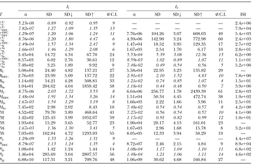
samples. The results are summarized in Table 1. For each relationship and each importance-sampling method we report the following: a, the mean a esti-mated over 100 replicate Monte Carlo simulations (this is equivalent toaestimated withN¼10 million); SD, the standard deviation of the 100 estimates ofacalculated from their observed distribution; SDY, the minimum, over the 100 replicate simulations, of the Monte Carlo standard errors of the estimates of a computed from the 100,000 Monte Carlo samples; SD[, the maximum SD over the 100 replicate simulations; and ;C.I., the number, out of 100 Monte Carlo simulations withN¼
100,000, that failed to includeain the 90% confidence interval for the estimate of a. ;C.I. should be close to 10.
The results (Table 1) show that, for most relation-ships, at least one of either I1orI2performs well. For
each true relationship, the results for the best-performing importance-sampling method appear in italics (i.e., for Figure3.—The relationship between false-positive rates,a, and power, 1 b, for minor allele frequency, q¼0.2, and number of loci,L¼80, at different values of the genotyping error rate,m. Note that they-axis is on a log scale. Each solid curve represents the relationship for a value ofm¼2nwith
each relationship type, the importance-sampling method in italics is the one that should be used in practice). It is apparent thatI1performs best in trios in which the
members are not highly related (i.e., when a putative parent was related no more closely than as a full-sibling to a true parent or as a half-sibling to y), and I2
out-performsI1when members of the trios are more closely
related (i.e., when only a single putative parent is a true parent or when a putative parent is a full-sibling of y). In most cases, the best importance-sampling method was able to estimateawith a standard error of between 0.5 and 2% usingN¼100,000, which takes,10 sec of user time on a 1.25-GHz G4 Apple laptop. The only excep-tions were relaexcep-tionship CU
Se, which could only be
estimated to a standard error of 5%, but could still be reliably estimated, and the relationshipsBU,D3,D5, and PH, for whichacould not be accurately estimated using
eitherI1orI2. It is probable that a different
importance-sampling scheme tailored to those relationships could
be devised that would work better, but we do not pursue that here. In the rest of this article, we either exclude those relationships from subsequent analyses or note results for them with caution.
The ‘‘ISI’’ column in Table 1 gives the approximate factor by which importance sampling decreases compu-tation time compared to the naive Monte Carlo estima-tor of Equation 6. This value is obtained by calculating the size of the Monte Carlo sample N that would be needed if using the naive Monte Carlo estimator to achieve the same Monte Carlo standard error foraand then dividing that by 100,000. For the 60-locus condi-tions we considered, the importance-sampling method is between 3.9 times and 44 million times faster, depend-ing on the relationship. The speed improvement due to importance sampling is greater for smaller values ofa
and will hence be greater for larger numbers of loci, for values ofacorresponding to higher values ofb, and for more distantly related trio members. In many cases
TABLE 1
Assessment of the importance-sampling methods
I1 I2
T a SD SDY SD[ ;C.I. a SD SDY SD[ ;C.I. ISI
CU
U 5.23e-08 0.89 0.92 0.95 9 — — — — — 2.4e106
CU
DFC 7.82e-07 1.27 1.09 1.35 13 — — — — — 7.9e104
CDFC
DFC 1.29e-05 1.20 1.06 1.24 11 7.76e-06 104.26 3.07 608.03 49 5.4e103 CU
Si 8.76e-06 2.20 1.80 4.47 6 4.39e-06 142.90 3.24 772.98 60 2.4e103
CDFC
Si 1.49e-04 1.57 1.34 2.47 9 1.47e-04 18.52 3.95 129.35 17 2.7e102
CSi
Si 1.66e-03 1.46 1.29 2.08 6 1.67e-03 2.54 1.70 6.17 10 2.8e101
CU
Se 5.43e-04 14.72 4.34 67.70 24 5.53e-04 5.39 3.08 12.36 13 6.2e100 CDFC
Se 8.57e-03 6.02 2.76 30.61 12 8.59e-03 1.02 0.89 1.07 11 1.1e101 CSi
Se 7.49e-02 3.25 1.89 9.92 9 7.48e-02 0.49 0.54 0.56 5 5.2e100
BU 5.08e-04 24.40 4.82 137.21 27 5.58e-04 22.95 3.23 135.82 29 — BDFC 2.76e-03 23.99 5.09 137.72 22 2.91e-03 2.10 1.52 4.83 10 7.8e100 BSi 1.14e-02 54.21 4.28 508.81 33 1.21e-02 0.74 0.85 1.07 4 1.5e101 BSe 1.04e-01 204.62 4.04 1859.42 58 1.18e-01 0.44 0.48 0.50 7 3.9e100
HU 8.75e-06 2.03 1.72 3.53 8 6.64e-06 256.77 1.78 2439.39 61 2.8e103
HDFC 1.48e-04 1.91 1.34 3.26 14 1.51e-04 50.34 4.45 472.74 38 1.9e102
HSi 1.67e-03 1.54 1.29 3.19 8 1.66e-03 2.22 1.66 3.96 11 2.5e101
HSe 7.45e-02 2.98 2.02 8.43 10 7.48e-02 0.54 0.54 0.57 8 4.2e100
D1 4.52e-02 79.70 3.89 468.64 41 7.27e-02 0.56 0.54 0.57 10 4.1e100
D2 1.42e-02 125.43 3.99 1052.07 59 1.17e-02 0.91 0.82 0.99 12 1.0e101
D3 1.93e-04 15.29 3.65 52.77 23 1.90e-04 20.17 4.13 161.01 23 —
D4 1.67e-03 1.36 1.30 3.41 5 1.67e-03 2.96 1.68 15.78 8 3.2e101
D5 7.03e-05 162.84 4.72 1293.03 55 8.05e-05 12.33 3.94 58.29 19 —
PU 1.29e-09 1.33 1.26 1.31 9 — — — — — 4.4e107
PDFC 8.79e-07 1.13 1.24 1.35 4 8.72e-07 2.46 2.15 4.84 9 8.9e104
PSi 1.08e-04 1.42 1.24 1.44 14 1.08e-04 1.17 1.04 1.10 11 6.8e102
PF 1.46e-04 285.69 3.04 2807.57 56 1.48e-04 1.21 1.06 1.11 14 4.6e102 PH 6.88e-10 117.31 3.21 709.76 48 1.06e-09 30.62 4.68 166.84 27 —
For different relationships, given in theTcolumn, 100 independent Monte Carlo estimates ofacorresponding tob¼0.1 were made using both methodsI1andI2. Results forI1appear on the left and those forI2on the right. The description of the quantities
given in the columns headed bya, SD, SDY, SD[, and;C.I. is given in the text. Values for the best-performing
importance-sampling method are in italics. For four relationships—BU,D3,D5, andPH—neitherI1norI2provided an acceptable reduction in
for whichI2is the best importance-sampling method,
the improvement from importance sampling is mar-ginal, primarily because the false-positive rates are high enough that estimating them with (6) is quite feasible.
Power of the likelihood-ratio method:For the 19 trio relationships and four paternity inference scenarios for which eitherI1orI2works well, we computedaatb¼
0.1, assumingm¼0.005, usingLloci withq¼0.2, where
L ranged from 20 to 120 in steps of 20. The results appear in Figure 4, in whichais plotted againstLfor each relationship. It is immediately clear that log a
decreases linearly withL, soadecreases exponentially withL. In practical terms this means that, as more SNP loci are available, it should be possible to perform accurate parentage inference in ever larger popula-tions. The slope of the line for each relationship tells how much extra information is available from each locus. For example, forCU
U trios, the slope of the line is 0.125, which means that an additional 10 loci will decrease the false-positive rate by a factor of 101030.125¼
17.8, and an additional 24 loci will decrease the false-positive rate by a factor of 1000. As can be seen in the plot, withL¼100, the false-positive rate forCU
U trios is
extremely low—only 4.631013. By contrast, the slope
of the line for trios of typeBSeis only0.0126, so even an
additional 24 loci will decrease the false-positive rate for such relationships only by a factor of 2. And, even with 100 loci,a¼0.037 for a trio in which the putative father is the true father and the putative mother is a sister of the putative offspring. This difficulty of distinguishing siblings from parents is not unique to SNPs and has been investigated by Thompsonand Meagher(1987).
In general,aincreases as the degree of relatedness between the members of a trio increases (Figure 4), as
expected. The pairsD1 andHSe,D2 andBSi, andD4 and HSi all have false-positive rates that are similar to one
another. For the first two pairs, this happens to be coincidental, but forD4 andHSi, at all values ofmandq,
the false-positive rates are identical. This is because, with unlinked markers,P(GjD4)¼P(GjHSi) for all
genotypic configurationsG, although they are different relationships.
For a particularbthe false-positive rate is minimized at a minor allele frequency of 0.5. This is a special case of the well-known result that, on average, a locus is most informative for relationship estimation when its alleles are equifrequent (Thompson1975). Were we to replot
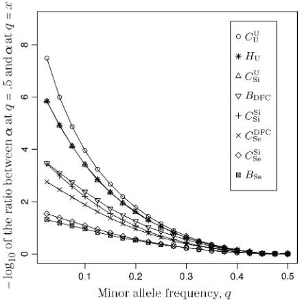
Figure 4 usingq¼0.5 we would find it to look much the same as before, but the slopes of all of the lines would be steeper. In Figure 5, the effect of allele frequency onais presented for eight different relationships. It is in-teresting to note that the beneficial effect of increasing the minor allele frequency of the SNPs used is greater at low frequencies than at high frequencies. For example, little additional power is gained by increasingqfrom 0.4 to 0.5 for all relationships.
Comparison to exclusion-based methods: We calcu-lated the false-positive and false-negative rates achieved by the exclusion method with 100 loci and then cal-culated how many loci would be required to achieve the sameaandbusing the likelihood-based method. This procedure was performed assuming thatm¼0.005 and that the minor allele frequency of all loci was 0.20, 0.35, or 0.50. It was repeated for all 22 trio relationship types. The exclusion criterion used was that of declaring a trio to be a parental trio only if ,2 of 100 loci were observed to be incompatible with Mendelian inheri-tance in the trio. This method of allowing a small Figure4.—aas a function of number of loci. Thex-axis plotsL, the number of loci having minor allele frequencyq¼0.2. The y-axis gives values ofaatb¼0.1 for the different relationships. Genotyping error ratemis assumed to be 0.005.awas computed by importance sampling, usingN¼100,000, for values ofLbetween 20 and 120 in steps of 20. Vertical bars at each value ofLused show the 90% confidence interval around the estimateda. For most relationships these vertical lines are imperceptible because the importance-sampling algorithms work well (they are most apparent along the line for relationshipCU
Se). Note that they-axis is
number of incompatible loci, to account for mutations or genotyping errors, is common practice in forensic paternity inference (Funget al.2002). The calculation
of exclusion probabilities is standard, but is repeated here for explicitness. LettingXdenote the number of loci, ofL, exhibiting Mendelian incompatibilities in a trio of relationshipT, it is apparent that, if the allele frequencies and genotyping error rates are constant across all loci, thenXBinomial(L,v), wherevis the probability that a locus is incompatible with Mendelian inheritance. In the notation of (A2) we have
v¼ X
0#gmð‘Þ;g
ð‘Þ
f ;g
ð‘Þ
y #2
I fPðgyð‘Þjgmð‘Þ;gfð‘ÞÞ ¼0g
3Pðgmð‘Þ;g ð‘Þ f ;gð
‘Þ y jT;mÞ;
wherePðgð‘Þ m ;g
ð‘Þ f ;g
ð‘Þ
y jT;mÞis computed assuming that m¼0.005, andI fPðgð‘Þ
y jg ð‘Þ m ;g
ð‘Þ
f Þ ¼0gis computed
as-suming thatm¼0. Hence, it is straightforward to com-putebExc¼P(X.1jQ) andaExc(T)¼P(X#1jT).
Form¼0.005 andq¼0.20, 0.35, or 0.50,bExcwith 100
loci is 0.80, 0.82, or 0.83, respectively.
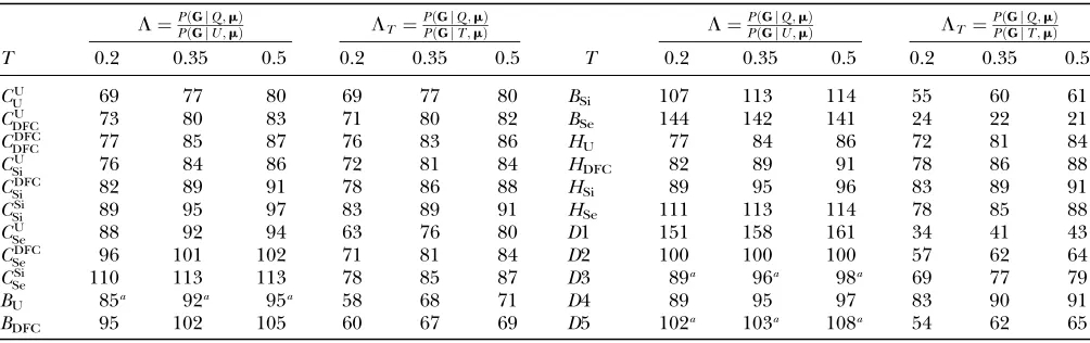
Table 2 contains the results of these comparisons. In all cases, the number of loci required of the likelihood method to achieveexactlythe samea andbas the ex-clusion approach would be a noninteger value. This value was approximated by interpolating between the
nearest consecutive integer values of the number of loci, and the results shown in Table 2 are rounded to the nearest integer. Two important trends are apparent. First, the likelihood method realizes greater improve-ments over the exclusion method for trios in which the individuals are not highly related to one another. Second, the benefit of conducting likelihood inference increases as the allele frequency decreases. For distin-guishing CU
U trios from parental trios, it requires ,70
loci atq¼0.2 to achieve the same performance that the exclusion method achieves with 100 loci.
For 13 of the 22 relationships, the likelihood method usingL¼PðGjQ;mÞ=PðGjU;mÞis clearly preferable to the exclusion method. For the remaining 9 relation-ships, however, the exclusion method performs as well or better than the likelihood method. The results forBSe
andD1 are particularly striking—the likelihood method may require as many as 144 or 161 loci to achieve the same power as the exclusion method with 100 loci. This can occur, because, as mentioned inmethods, when the
true relationship is notU(orCU
U, as we have been calling
it), then there is no guarantee that a likelihood-ratio test based onL¼PðGjQ;mÞ=PðGjU;mÞis the most power-ful test available. This observation is related to the para-doxical phenomenon encountered in the estimation of pairwise genealogical relationships in which ‘‘bilateral relatives such as full-sibs may be more likely parents than the true parent individuals’’ (Thompsonand Meagher
1987, p. 585).
Thompsonand Meagher (1987) showed that the
discrimination of pairwise parent–offspring and sibling– sibling relationships can be improved by jointly consid-ering the two likelihood ratios that arise by using either the likelihood of the parent pair or that of the sibling relationship in the numerator. In a similar way, it is pos-sible to use a combination of different likelihood ratios to more efficiently discriminate parental trios from other trios with closely related members. The Neyman– Pearson lemma indicates that the most powerful statistic for distinguishing a trio of typeTfrom a trio of typeQ
would beLT ¼PðGjQ;mÞ=PðGjT;mÞ. Table 2 shows that forBSeandD1—the two relationships for which the
likelihood method seems to work poorly relative to exclusion—usingLT allows the likelihood method with as few as 21 and 34 loci, respectively, to perform as well as exclusion with 100 loci. In general, usingLTseems most
advantageous in situations in which one (or both) of the putative parents of the trio is a full sibling of the putative offspring. It thus seems likely that a test statistic that is a combination of bothPðGjQ;mÞ=PðGjU;mÞand
LT for one or a variety of trio relationships, T, could
offer a more powerful likelihood approach when some of the trios are expected to include highly related in-dividuals such as full siblings. Of course, as pointed out by Thompsonand Meagher(1987), the utility of
such an approach depends on the correlation between
LandLT. Figure5.—The effect of allele frequency on false-positive
rates.L¼60 SNPs with minor allele frequency as given on the
x-axis were simulated andawas computed for the eight rela-tionships listed in the inset. They-axis is the negative log to the base 10 of the ratio betweenaatq¼0.5 (the minimum value ofa) andawithqas given on thex-axis. For example, for theCU
U relationship, the false-positive rate for 60 loci is
An example:To illustrate the scale of study that is pos-sible, we consider the prospects for large-scale parent-age inference to infer the mothers and fathers of a cohort born in a large, hypothetical, chinook salmon population. Using the program spip (Anderson and
Dunham 2005) we simulated a population of roughly
constant size in which an average of 3820 females and 3540 males return to their natal stream each year to spawn and die. Of the male spawners, an average of 28, 57, and 15% were 3-, 4-, and 5-year-olds, respectively. Of the females, on average, 79% were 4-year-olds, and the rest were 5-year-olds. Female mate fidelity was set so that most females had fewer than four male mates (thus creating many more full-sibships than would occur if mating were at random) and the variance in reproduc-tive success of males and females was set so that the effective number of spawners was roughly one-quarter of the census number of spawners (Wapleset al. 1993).
This serves to create larger families than expected under Wright–Fisher-like reproduction, thus increasing the degree of relatedness between individuals in the population. The population was simulated forward in time, starting at year40. At year 0 we simulated the nonlethal collection of genetic data from all males and females returning to spawn (3825 females and 3450 males). Such sampling could occur, for example, if all the fish had to pass through a weir or fish ladder before spawning. At years 3, 4, and 5, we simulated genetic sampling of all spawning adults—21,819 in all. Of those fish, 7336 were offspring of the parents genotyped in year 0, and the rest were offspring of fish that spawned in years2,1, 1, or 2. We then imagined that parentage
was to be inferred by comparing each of the 21,819 fish from years 3 to 5 to all possible pairs of the 3825 females and 3450 males that spawned in year 0—a total of 21,81933825334502.931011trio comparisons.
We assumed 100 SNPs withq¼0.2 andm¼0.005. Our goal was to estimate the total number of false-positive and false-negative errors expected in conducting such a study. To do this, we first had to calculate the number of trios of different relationship categories that would be encountered. This was achieved by enumeration of the relationships between the putative parents at year 0 and all the true parents of individuals spawning in years 3–5. This approach explicitly takes account of the effects of variation in family size on the distribution of such rela-tionships. Any individuals sharing ancestors more than two generations apart were considered to be unrelated— a reasonable assumption given that the effect of such distant relationships on the distribution ofLis minimal. Because of the semelparous nature of salmon, and the age structure of their populations, the only types of trios that will be encountered are of theCcategory. Enumer-ating the relationships between the true and the puta-tive parents we found the vast majority, 99.8%, of trios to be of typeCU
U, with the remainder of the trio categories
involving pairwise relationships of Se, Si, half-sib (HS), first cousin (FC), and half-cousin (HC). The latter three relationships have not been previously considered in this article, but are dealt with in a similar manner using their coefficients: for HS, k¼ ð1
2; 1
2;0Þ; for FC, k¼
ð3 4;
1
4;0Þ;and for HC, k¼ ð 7 8;
1
8;0Þ. A small proportion of trios included putative parents related in aunt–niece or other relationships. These relationships were not
TABLE 2
Number of loci required for the likelihood-ratio method to achieve the sameaandbas 100 loci using an exclusion-based method
L¼PPððGGjjQU;;mmÞÞ LT ¼P
ðGjQ;mÞ
PðGjT;mÞ L¼
PðGjQ;mÞ
PðGjU;mÞ LT ¼P
ðGjQ;mÞ
PðGjT;mÞ
T 0.2 0.35 0.5 0.2 0.35 0.5 T 0.2 0.35 0.5 0.2 0.35 0.5
CU
U 69 77 80 69 77 80 BSi 107 113 114 55 60 61
CU
DFC 73 80 83 71 80 82 BSe 144 142 141 24 22 21
CDFC
DFC 77 85 87 76 83 86 HU 77 84 86 72 81 84
CU
Si 76 84 86 72 81 84 HDFC 82 89 91 78 86 88
CDFC
Si 82 89 91 78 86 88 HSi 89 95 96 83 89 91
CSi
Si 89 95 97 83 89 91 HSe 111 113 114 78 85 88
CU
Se 88 92 94 63 76 80 D1 151 158 161 34 41 43
CDFC
Se 96 101 102 71 81 84 D2 100 100 100 57 62 64
CSi
Se 110 113 113 78 85 87 D3 89a 96a 98a 69 77 79
BU 85a 92a 95a 58 68 71 D4 89 95 97 83 90 91
BDFC 95 102 105 60 67 69 D5 102a 103a 108a 54 62 65
TheTcolumn denotes the true relationship of the trio. For each relationship, there are six columns. The first three columns give the number of loci required to have a and b comparable to the exclusion method when using the test statistic L¼PðGjQ;mÞ=PðGjU;mÞand whenq¼0.2, 0.35, and 0.5 as indicated by the column headings. The fourth through sixth columns to the right of each relationship show the number of loci required for a test of relationshipT vs. relationshipQ, based onLT ¼PðGjQ;mÞ=PðGjT;mÞ(the most powerful test statistic that could be used if all the trios were knowna priorito be either of typeQor of typeT), to have the sameaandbas the exclusion-based method.
a
only rare, but they also did not contribute to the overall false-positive rate, so we do not include them in the results. We used (5) to chooseLc¼22.79 to yield a
false-negative rate ofb¼0.051.
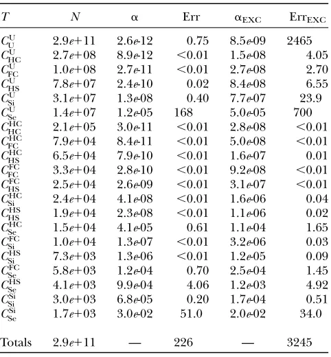
Overall, the prospects for parentage assignment in such a large population are promising (Table 3). Of the 7336 sampled offspring of the males and females genotyped at year 0, the expected number assigned to their parents is (1b)37336¼6962. Of the 2.931011
trios that were not of typeQ, 226 are expected to have
L . Lc ¼ 22.79. All but approximately one of these
expected incorrect assignments will involve one correct parent. Hence, 94.9% of 225 expected, misassigned offspring are expected to also belong to correctQtrios havingL.Lc¼22.79. To be conservative, all offspring
associated with .1 trio having L . Lc could be
dis-carded as having unidentified parents. This would leave 6748 offspring expected to be correctly assigned to their parents and 13 offspring expected to be incorrectly assigned; i.e., ,2 of 1000 assignments of offspring to parents are expected to be incorrect.
Table 3 also provides the numbers of misassigned offspring expected in the study if an exclusion-based criterion is used. In this case, excluding trios if they carry more than two loci with Mendelian incompatibilities leads to a false-negative rate ofbEXC¼0.051—identical
to the false-negative rate used above in estimating error rates using the likelihood-based method. Using this exclusion-based criterion, 2465 of theCU
U trios are
ex-pected to be incorrectly classified as parental trios. The other expected misassignments include 38 trios that do not include either correct parent and 742 trios in which there is at least one correct parent. If one were to apply the same conservative rule of excluding offspring that are nonexcluded from more than one parent pair, then parentage would be assigned to246513816962
74230.949¼8761 offspring. Of these, 74230.0511
2465138¼2541 are expected to be incorrect. Thus,
2541/8761 29% of assigned offspring would be assigned to an incorrect parent pair using an exclusion-based method. This number overestimates the true ex-pected number, somewhat, because it does not account for the fact that some fraction of the 2541 incorrectly assigned offspring is expected to be assigned to more than one incorrect parent pair. Nonetheless, it clearly makes the point that the likelihood-based approach is far more powerful than the exclusion-based approach in a population where most parents are unrelated.
DISCUSSION
We predict that SNPs will quickly become the marker of choice for parentage inference in populations of heavily managed species, as well as for large populations, because SNPs are well suited to the high-throughput genotyping required of large studies and because SNP genotyping error rates are low. The advantages of SNPs are particularly apparent in situations where multiple laboratories collaborate on the genotyping effort, and standardization of microsatellite allele calls across all the labs would be costly or infeasible. In this article we provide several advances that allow the application of likelihood-based methods to large-scale parentage in-ference using SNPs. We describe two importance-sampling algorithms that make the calculation of small false-positive rates, in the presence of genotyping error, computationally feasible. We show that the importance-sampling methods work well for a range of trio types, but do not work well for some cases involving putative parents that are full- or half-siblings of the youth. De-veloping an efficient importance-sampling algorithm for those cases (BU,D3,D5, and PH) remains an open
problem. For trios involving unrelated individuals, the importance-sampling method is millions of times faster than a naive Monte Carlo estimator, even with as few as 60 loci. Although we have focused on SNPs, both importance-sampling algorithms could be modified to handle cases involving other, multiallelic loci.
TABLE 3
Numbers of trios of different types, per-trio false-positive rates, and expected total numbers of false positives
for the hypothetical chinook salmon study described in the text
T N a Err aEXC ErrEXC
CU
U 2.9e111 2.6e-12 0.75 8.5e-09 2465 CU
HC 2.7e108 8.9e-12 ,0.01 1.5e-08 4.05 CU
FC 1.0e108 2.7e-11 ,0.01 2.7e-08 2.70 CU
HS 7.8e107 2.4e-10 0.02 8.4e-08 6.55 CU
Si 3.1e107 1.3e-08 0.40 7.7e-07 23.9 CU
Se 1.4e107 1.2e-05 168 5.0e-05 700 CHC
HC 2.1e105 3.0e-11 ,0.01 2.8e-08 ,0.01 CHC
FC 7.9e104 8.4e-11 ,0.01 5.0e-08 ,0.01 CHC
HS 6.5e104 7.9e-10 ,0.01 1.6e-07 0.01 CFC
FC 3.3e104 2.8e-10 ,0.01 9.2e-08 ,0.01 CFC
HS 2.5e104 2.6e-09 ,0.01 3.1e-07 ,0.01 CHC
Si 2.4e104 4.1e-08 ,0.01 1.6e-06 0.04 CHS
HS 1.9e104 2.3e-08 ,0.01 1.1e-06 0.02 CHC
Se 1.5e104 4.1e-05 0.61 1.1e-04 1.65 CFC
Si 1.0e104 1.3e-07 ,0.01 3.2e-06 0.03 CHS
Si 7.3e103 1.3e-06 ,0.01 1.2e-05 0.09 CFC
Se 5.8e103 1.2e-04 0.70 2.5e-04 1.45 CHS
Se 4.1e103 9.9e-04 4.06 1.2e-03 4.92 CSi
Si 3.0e103 6.8e-05 0.20 1.7e-04 0.51 CSi
Se 1.7e103 3.0e-02 51.0 2.0e-02 34.0
Totals 2.9e111 — 226 — 3245 TheTcolumn gives the relationship of the trio. TheN col-umn gives the number of such trios among the 2.931011trios
compared in the study. Theacolumn gives the false-positive rates, and the ‘‘Err’’ column gives the total expected number of parental misassignments expected from each trio category when using a likelihood-based assignment method. The value in the Err column is the product of the values in theNanda columns. The aEXC and ErrEXC columns show the results
We present simulations demonstrating that likelihood-based inference of parentage may be considerably more efficient than a method based on the exclusion of trios with an excess of Mendelian incompatibilities. In the case of totally unrelated trios, the likelihood method can achieve the same power and accuracy as the ex-clusion method with 30% fewer loci. Another way of stating this result is that, for distinguishing unrelated trios from parental trios, the method of exclusion could require up to 143 loci to perform as well as the likelihood-based method with 100 loci. Since most of the trios compared in a large study will likely be un-related (as shown in the salmon example), this greater efficiency of the likelihood method is particularly ger-mane. However, for trios involving one correct parent and a sibling of the other parent, as well as for trios in which one putative parent is a full-sibling of the youth itself, the method of exclusion performs better than the likelihood method. This argues for the application, when such situations are likely, of a hybrid approach in which trios are initially compared on the basis of the standard likelihood ratio for parentage [PðGjQ;mÞ=
PðGjU;mÞ], and all those having Lgreater than the critical value, Lc, should be investigated further,
per-haps by applying an exclusion-based test or perper-haps by using a statistic like LT described in this article. The latter would be a sort of sequential version of the method recommended in Thompson and Meagher
(1987) for dealing with the case where full-siblings of the youth are putative parents. Such a sequential pro-cedure would have to be designed carefully so that the overall false-positive and false-negative rates could still be reliably calculated.
We have given a brief summary of the false-positive rates that can be expected using different numbers of SNP loci. We show that false-positive rates decrease exponentially with the number of loci. The conse-quence of this is that one typically requires only a modest increase in the number of loci to accommodate even a rather large increase in the number of potential parents and offspring in a study. This feature, combined with the fact that SNPs are abundant in the genome of most organisms (Brumfield et al. 2003), is
encourag-ing. Our calculations show that false-positive rates for unrelated trios can be extremely small with a moderate and feasible number of SNP loci. Unfortunately, for closely related trios, particularly those in which a full-sibling of the offspring is a putative parent, the false-positive rates, even with a large number of loci, can be high, especially if one of the putative parents is, indeed, the correct one. This problem is not unique to parent-age inference with SNPs, but, in fact, exists for all genetic marker systems (see, for example, Thompson
and Meagher 1987). Fortunately, in some contexts,
occurrence of such closely related trios will be quite rare. This is particularly true in studies of large pop-ulations, as our salmon population example
demon-strates. However, nonparental trios containing highly related members may be a substantial problem in some situations, such as small populations, species with ex-tremely high variance in reproductive success, or pop-ulations that have recently experienced a reduction in effective size.
The method of parentage inference described here requires that independent estimates of the genotyping error rate be available for all loci or that some reason-able genotyping error rates can be assumed. In the absence of any prior knowledge about true parental relationships, it would not be possible to jointly estimate the genotyping error rate and the relationships. De-creasing the genotyping error rate decreases the false-positive rate at a given false-negative rate. The power analyses described here were done assuming a per-gene-copy genotyping error rate of 0.5%. This value is at the very upper end of reported genotyping error rates for SNPs, and it still provides ample power for parentage inference. Also, SNPs with a minor allele frequency of 0.5 provide the most power for parentage inference, although little additional power is gained aboveq¼0.4. In many of the simulations, we usedq¼0.2, so it should be kept in mind that comparable power could be achieved with fewer loci if they are selected such that
q.0.2.
Throughout our simulations we have assumed that the allele frequencies among the parents are known without error. For large studies, involving thousands of parents, this is a reasonable assumption because, unless they are all descended from a small number of individ-uals, the large sample of parents should provide an excellent estimate of the allele frequencies. It should also be pointed out that, since parentage inference is not concerned with the inference of evolutionary his-tory, the ascertainment of SNPs through discovery in particular populations or genomic regions (Wakeley et al. 2001) does not bias the results of parentage in-ference in any way. In fact, SNP ascertainment leads to an advantage in parentage inference because ascertain-ment typically leads to an overrepresentation of SNPs at intermediate allele frequencies—exactly the type of loci that are most powerful for parentage.
managed species. Our example of a large salmon pop-ulation reflects this—given good information about age structure and family size variance, a reasonable approx-imation of the distribution of trio relationships in a population can be obtained. We reiterate here that salmon populations are special in that all trio relation-ships will be of aCf
mtype. To efficiently compute
false-positive rates of randomly drawn trios from more generally structured populations may require devising specialized importance-sampling algorithms for theBU, D3, D5, and PH relationships. This remains an open
problem.
An argument that has been made against the use of SNPs in the estimation of relationships is that, since so many SNPs are required, there is high probability that some of them will be physically linked, and that genetic linkage may not even be recognized because the mark-ers may not be in linkage disequilibrium (see, for ex-ample, Glaubitzet al.2003). There are two important
points to be made with regard to the effect of linkage and LD on parentage inference. First, as has been pointed out previously (Chakraborty and Hedrick
1983; Jonesand Ardren2003), LD will always decrease
the per-locus power for parentage inference, because each locus no longer provides independent informa-tion. Consequently, whenever possible, SNPs used for parentage inference should be chosen to have no sig-nificant LD. This should not be difficult, even for physically linked SNPs, since LD has been observed to drop to low values over physical distances of,200 kb (Pritchard and Przeworski 2001). Second, in the
absence of LD, the effect of physical linkage on par-entage inference depends on the true relationship of the individuals in the trio. Most importantly, for all trios of theCf
mtype, physical linkage without LDdoes not affect
the distribution ofL. Therefore, for example, physical linkage (with no LD) is irrelevant in the analysis of mother–father–youth trios in a salmon population, where only trios of theCf
mtype are possible. This is true
because, with no LD, the probabilityP(Gj Cf
m) is the
same whether or not alleles occur together on the same haplotype, because there is no information available in
Cf
m-type trios to infer the haplotypic phase of alleles that
are heterozygous in all trio members.
Physical linkage does, however, affect the distribution of L for trios in which two members may have each inherited genetic material from a single founder of the pedigree that connects the trio members (i.e., theB,H, andDtrio types). Although the mean of the distribution ofLremains unchanged, physical linkage increases the variance of the distribution for such trios. Accordingly, false-positive rates calculated for such trios under the assumption of no linkage (as examined here) will underestimate the true false-positive rate in the pres-ence of linkage. One solution to this problem would be to simulate the genetic data using a method that ex-plicitly takes account of the linkage. However,
develop-ing an importance-sampldevelop-ing scheme to make this type of simulation efficient with many linked markers might be difficult. Additionally, for trio types in which physical linkage affects the distribution of L, a more powerful test statistic thanLcould be derived that took account of the linkage. Such a method could build upon the framework of Sieberts et al.(2002), but requires that
estimates of the recombination fraction between markers are available.
We have focused on the estimation of false-positive rates and their use in calculating expected studywide error rates. Such calculations are useful for guiding study design and determining the number of loci re-quired to achieve a certain degree of reliability. They do not, however, address the actual practice of carrying out the trio comparisons. As pointed out by Meagherand
Thompson(1986), comparing all offspring to all possible
parent pairs could be computationally prohibitive— performing 1011trio comparisons is extremely time
con-suming. Fortunately, this computational burden can be reduced by a number of strategies. We will provide de-tails in a separate article, but we note here that the num-ber of trios for which the likelihood must be evaluated can be significantly reduced by first excluding individ-ual males and females from consideration by using a nonstringent (i.e., having a low false-negative rate) ex-clusion criterion based on large numbers of Mendelian incompatibilities. This is computationally advantageous with SNPs because assessing Mendelian incompatibility for many loci at once can be done rapidly by employing bitwise logic operations. Furthermore, for searches of large databases of parents, a suffix tree (McCreight
1976) representation of the genotypes of males and females would allow rapid identification of nonex-cluded parents, and the problem of identifying parents or parent pairs sharing zero, or a small number, of Mendelian incompatibilities with any individual can be translated into a special case of the approximate keyword search problem, for which fast algorithms are known (Myers1994).
We also note that we have not addressed several other improvements to the practice of large-scale parentage inference that could be made. For example, in large studies, it is likely that some males or females will have more than one offspring assigned to them. After a pre-liminary inquiry based on trios, larger family groups could be analyzed as a unit to provide sharper parentage inferences, reducing the false-positive rate. However, it should be noted that many such comparisons (i.e., those involving multiple potential children of the same parent or parent pair) will be affected by physical linkage, even in the absence of LD.
We distribute two computer programs written in C implementing the calculations presented in this article.