ABSTRACT
ROTHFUSS, NICHOLAS ERNEST. Toward Better Characterization of the Viscosity of Organic Aerosol. (Under the direction of Dr. Markus D. Petters).
Atmospheric aerosol is central to various processes of meteorological or climatological concern and is a pollutant of significant concern for human health. Much of the particulate matter present in the atmosphere is composed of organic compounds. Organic aerosol (OA) can be liquid-like, semi-solid, or have mechanical properties similar to a glass, a difference of
approximately 15 orders of magnitude in measured viscosities. Modelling studies suggest that highly viscous OA will be common in the middle and upper troposphere and in drier and colder regions of the lower troposphere. At near-glassy viscosities, bulk diffusion within the particle may be sufficiently inhibited as to render assumptions of rapid equilibration between the particle and its ambient environment during processes such as hygroscopic growth invalid, and thus serve as a potential source of error in cloud and climate models. Viscous outer shells may shield
reactive species in the particle bulk from reaction with ambient oxidant species or inhibit evaporation of volatile species initially present within the bulk, dramatically increasing the atmospheric lifespan of such compounds and thus can provide a long-range transport mechanism for toxic or carcinogenic substances such as polycyclic aromatic hydrocarbons. Finally, highly viscous OA particles may serve as ice nuclei, altering pathways of cirrus cloud formation and concomitant radiative effects. Accordingly, there is scientific merit in quantifying OA viscosity and characterizing the processes that drive it and are modulated by it.
groups modulate viscosity and/or glass transition temperature of atmospherically relevant compounds, based upon data collated from literature. Chapter 3 demonstrates a method for probing the viscosity of nanoscale aerosol by using measurements of apparent electrical mobility diameter to assess the morphology of dimerized particles subject to a brief period of
conditioning. Chapter 4 presents a phase diagram model for binary aqueous aerosol, using sucrose as the representative system. This model combines the Gordon-Taylor equation for representing the humidity-dependence of glass transition temperature, a modified Vogel-Fulcher-Tammann equation for representing the temperature-dependence of viscosity, and a mass-based water activity parameterization, with model parameters derived using viscosity measurements made with the experimental method of Chapter 3. Chapter 5 characterizes and defines minimum experimental parameters for the experimental method of Chapter 3. Finally, Chapter 6
investigates the relationship between initial particle viscosity and condensational growth kinetics for a number of aqueous carbohydrate systems commonly used as OA proxies, using a
Toward Better Characterization of the Viscosity of Organic Aerosol
by
Nicholas Ernest Rothfuss
A dissertation submitted to the Graduate Faculty of North Carolina State University
in partial fulfillment of the requirements for the degree of
Doctor of Philosophy
Marine, Earth, and Atmospheric Sciences
Raleigh, North Carolina 2019
APPROVED BY:
_______________________________ _______________________________ Dr. Markus D. Petters Dr. Andrew P. Grieshop
Committee Chair
ii BIOGRAPHY
I was born in Lexington, Kentucky, but grew up in Mount Pleasant, Michigan where my parents were both professors at Central Michigan University (CMU). Following high school, I attended Bowling Green State University in Ohio (not Kentucky, as is often mistakenly assumed), earning a Bachelor of Science degree (magna cum laude) with majors in both mathematics and computer science in December 2000. Flash forward a decade to the Fall of 2010, and I was working as a freelance web developer. It was becoming abundantly clear that I did not have the necessary passion for the business side of freelancing and something new was necessary. So, I applied for a job at the local bank and in one of those keystone moments of life that only appear pivotal in hindsight, I was not hired. On to the next idea. As long as I can remember, I have always been fascinated with the weather. At the time, I was living in Harrison, Michigan, which is in commuting distance of CMU, which so happens to have the state of Michigan’s only undergraduate meteorology program, in which I enrolled in January of 2011. As is typical of such programs, CMU’s meteorology major has a general chemistry requirement. As I fulfilled this during the Summer of 2011, it became clear to me that my interest in chemistry might be every bit as strong as my interest in meteorology, so I added it as a second major. A bit later, in the Summer of 2013, I was a volunteer student intern at the National Weather Service office in Gaylord, Michigan, during which I realized I was more interested in a research career than in weather forecasting. Thus, fusing my interests in meteorology and chemistry, I begin investigating graduate programs offering the chance to study atmospheric chemistry.
iii ACKNOWLEDGMENTS
I would first like to acknowledge my advisor, Dr. Markus D. Petters, for providing me with this opportunity, and my committee members: Dr. Andrew P. Grieshop, Dr. Yang Zhang, and Dr. Paul Ziemann.
Next, I would like to thank the credited co-authors on the papers comprising this dissertation: the aforementioned Dr. Petters and Dr. Greishop; Dr. Wyatt Champion of the Department of Civil, Construction, and Environmental Engineering; Dr. Sarah M. Petters of the University of North Carolina; and Dr. Jonathan P. Reid, Dr. Aleksandra Marsh, and Dr. Grazia Rovelli of the University of Bristol. Some of the work presented here would not have been possible at all without your collaboration, and everything presented here has been improved by it. Much credit also must be given to the post-doctoral scholar in our group, Dr. Timothy Wright, who never made it onto a byline of mine, but whose engineering savvy was always appreciated during experiment development and whenever technical issues would manifest with
instrumentation.
Of course, I would like to acknowledge the various funding agencies who have made the past five years possible: The National Science Foundation, the National Environmental Research Council of the United Kingdom, and particularly, the United State Department of Energy’s Atmospheric Systems Research program, which was the predominate funding source over the course of my Ph.D. work.
iv TABLE OF CONTENTS
LIST OF TABLES ... viii
LIST OF FIGURES ... xi
Chapter 1: Introduction ... 1
Possible Implications of Viscous Organic Aerosol ... 4
Organic Aerosol Formation and Ageing ... 8
Measuring Aerosol Viscosity ... 12
Modelling Aerosol Viscosity ... 18
This Dissertation ... 27
References ... 29
Chapter 2: Influence of Functional Groups on the Viscosity of Organic Aerosol ... 52
Abstract ... 53
Introduction ... 55
Materials and Methods ... 58
Results and Discussion ... 54
Hydroxyl Groups ... 60
Carboxylic Acid Groups ... 62
Nitrate Groups ... 65
Carbonyl and Ester Groups ... 65
Methylene Groups ... 66
Open Questions ... 66
Broader Implication ... 67
Associated Content ... 69
Supporting Information ... 69
Author Information ... 69
Corresponding Author ... 69
Author Contributions ... 70
Funding Sources... 70
Acknowledgements ... 70
References ... 71
Chapter 3: Coalescence-Based Assessment of Aerosol Phase State Using Dimers Prepared Through a Dual-Differential Mobility Analyzer Technique ... 89
Abstract ... 90
Introduction ... 91
Methods... 93
Viscosity Estimation ... 93
Experiment Type ... 95
Chemicals Used ... 96
Experimental Design ... 96
Temperature and Humidity Control ... 98
RH Sensor Calibration and Uncertainty ... 99
Data Collection and Processing ... 100
v
Experimental Results ... 102
Cooling Cycle (RH) Experiments ... 102
Sucrose Heating Cycle (Melting) Experiment ... 104
Discussion ... 105
Summary ... 107
Acknowledgements ... 108
References ... 109
Chapter 4: Characterization of the Temperature- and Humidity-Dependent Phase Diagrams of Amorphous Nanoscale Organic Aerosols ... 127
Abstract ... 128
Introduction ... 129
Methods... 132
Viscosity Measurements ... 132
Additional Viscosity Data ... 137
Viscosity Model ... 138
Sensitivity Analysis ... 140
Results ... 141
Discussion ... 146
Conclusion ... 152
Acknowledgements ... 153
References ... 154
Chapter 5: Characterization of a Dimer Preparation Method for Nanoscale Organic Aerosol ... 179
Abstract ... 180
Introduction ... 180
Methods... 184
DTDMA Characterization Experiments ... 184
Decharge-TDMA (DeDTDMA) ... 187
Radiation Sensitivity Experiment ... 188
Shielding Experiment... 188
Concentration Experiments ... 188
Residence Time Experiments ... 189
Flow Ratio Experiments ... 189
DCIC Characterization Experiments ... 190
Probe Monomers ... 190
Size Limitations ... 191
Modeling ... 191
Characterization of DTDMA Output ... 193
Monomer Decharging ... 193
Interplay of Mobility-Selected Concentration, Residence Time, and Decharging ... 195
Flow Ratio Effects ... 198
Signal Loss at Small Monomer Diameter ... 199
Specialized Dimer Characterization ... 201
vi
Probe Monomers ... 202
Resolution of Distinct Dimer Morphologies... 203
Conclusions ... 205
Acknowledgements ... 207
References ... 208
Chapter 6: Condensation Kinetics of Water on Amorphous Aerosol Particles ... 227
Abstract ... 228
Letter ... 228
Experimental Methods ... 237
Associated Content ... 238
Supporting Information ... 238
Author Information ... 238
ORCIDs... 238
Notes ... 238
Acknowledgements ... 238
References ... 239
Chapter 7: Summary ... 254
References ... 260
APPENDICES ... 261
Appendix A: Supporting Information: Influence of Functional Groups on the Viscosity of Organic Aerosol ... 262
Functional Group Model ... 263
Supplementary Tables S1-S5 ... 265
Supplementary Figures S1-S2 ... 337
References ... 339
Appendix B: Supplemental Information for “Coalescence-Based Assessment of Aerosol Phase State Using Dimers Prepared Through a Dual-Differential Mobility Analyzer Technique ... 386
The Viscosity Model ... 387
Curve Fitting ... 392
Supplementary Data ... 393
References ... 399
Appendix C: Electronic Supplementary Information for “Characterization of the Temperature- and Humidity-Dependent Phase Diagram of Amorphous Nanoscale Organic Aerosols... 400
Additional Figures Referenced in the Manuscript ... 401
Additional Tables Referenced in the Manuscript ... 415
vii Appendix D: Supplemental Information for “Characterization of a Dimer
Preparation Method for Nanoscale Organic Aerosol” ... 418
Additional Figures ... 419
Data Tables ... 423
Additional Discussion on Monomer Decharging ... 441
Additional Discussion on Particle Loss Mechanisms ... 442
Derivation of Geometric Parameters for the Mobility Diameter Models of Fig. 12 ... 444
Doublet of Spheres Geometry ... 445
Cylindrical Rod Geometry ... 445
Prolate Spheroid Geometry ... 446
References ... 448
Appendix E: Supporting Information for “The Condensation Kinetics of Water On Amorphous Aerosol Particles” ... 451
Electrodynamic Balance Experimental Methods ... 452
Gas Diffusional Growth Model ... 454
Calculation of Bulk Mixing Time ... 459
Mass Accommodation Coefficient ... 460
viii LIST OF TABLES
Chapter 2
Table 1 Glass transition temperatures for alcohols and acids with equal number of
functional groups ... 84
Chapter 3 Table 1 Observed relaxation RH values and literature deliquescence RH values for reagents considered in this work ... 118
Chapter 4 Table 1 Summary of measured and calculated temperature/RH combinations corresponding a sucrose viscosity of 5 x 10⁶ Paꞏs ... 169
Table 2 Summary of fitted sucrose viscosity model parameter values ... 170
Chapter 5 Table 1 Summary of experimental aerosol systems and preparation methods ... 214
Appendix A Table S1 Summary of compiled glass transition data ... 265
Table S2 Summary of literature viscosity data utilized, literature-derived viscosity values at 298.15 K used in functionalization sensitivity calculations, and model-estimated viscosity values at 298.15 K ... 275
Table S3 Fitted temperature dependence curves for laboratory viscosity data ... 298
Table S4 Calculated viscosity functionalization sensitivities ... 335
Table S5 Calculated vapor pressure functionalization sensitivities ... 336
Appendix B Table S1 Calculated geometries at various stages of coalescence as adapted from Table 1 in Pokluda et al. (1997) ... 390 Appendix C
ix work. Experiment numbering corresponds to order of mention in Table 1
of the main manuscript ... 415 Appendix D
Table S1 Abbreviations utilized in the tables of this section. Charge quantities relate to the charge on the particle in the final SMPS. ... 424 Table S2 Uncertainty reporting conventions utilized in the tables of this section ... 425 Table S3a Experimental data for Fig. 5a in the main manuscript ... 426 Table S3b Experimental data for Fig. 5b in the main manuscript. Coagulation time
includes estimated 6 second dwell time in the pre-mixing volume used for these experiments and an additional estimated 6 second dwell time elsewhere in the system between the exit to the mobility-selecting DMAs and the inlet to the electrostatic precipitator excluding the coagulator assembly. Shaded rows correspond to trials which deviated from the expected trend due to
irregularities at low flow ... 427 Table S4 Experimental data for Fig. 6b in the main manuscript ... 428 Table S5a Experimental data for unshielded trials in Fig. 7 in the main manuscript.
Coagulator residence time includes estimated 6 second dwell time in the pre-mixing volume used for these experiments and an additional estimated 6 second dwell time elsewhere in the system between the exit to the mobility-selecting DMAs and the inlet to the electrostatic precipitator excluding the coagulator assembly. Shaded rows correspond to trials which deviated from
the expected trend due to irregularities at low flow ... 429 Table S5b Experimental data for shielded trials in Fig. 7 in the main manuscript.
Coagulator residence time includes estimated 6 second dwell time in the pre-mixing volume used for these experiments and an additional estimated 6 second dwell time elsewhere in the system between the exit to the mobility- selecting DMAs and the inlet to the electrostatic precipitator excluding the coagulator assembly. Shaded rows correspond to trials which deviated from
the expected trend due to irregularities at low flow ... 430 Table S6a Experimental data for shielded trials in Fig. 8a of the main manuscript ... 431 Table S6b Experimental data for unshielded trials in Fig. 8a of the main manuscript ... 433 Table S7a Experimental data for the (approximately) constant upstream concentration
x
concentration trials in Fig. 9a of the main manuscript ... 435
Table S8a Experimental data for Fig. 11a in the main manuscript ... 436
Table S8b Experimental data for Fig. 11b in the main manuscript ... 438
xi LIST OF FIGURES
Chapter 2
Figure 1 Viscosity data (circles) and glass transition temperatures with two-standard deviation error bars (squares), and fitted VFT equation curves (including the glass transition) for 2-hexanol (red −1 OH), 1,2-pentanediol (orange −2 OH), 1,2,6-hexanetriol (magenta −3 OH), threitol (yellow −4 OH), xylitol (cyan −5 OH), sorbitol (dark blue −6 OH), and sucrose (black −8 OH). Data sources are listed in SI Tables S1 and S4. The gray shaded area corresponds to the
approximate range of temperatures of tropospheric interest ... 85 Figure 2 Viscosity data extracted from literature for alcohol (a), carboxylic acid (b),
carbonyl (c), ester (d), and organic nitrate (e) species at 298.15 K. Unfilled markers indicate the value was extrapolated while filled markers represent
interpolated data ... 86 Figure 3 Sensitivities of viscosity to functional group addition versus sensitivity
of vapor pressure (P) to functional group addition at 298.15 K. Red circles: both sensitivities were calculated from data. Blue circles with labels that end in a “?”: one sensitivity was calculated from data (viscosity for OH #3, vapor pressure for COOH #2), the other was extrapolated from an
approximate linear trend line fitted to the points where both sensitivities could be calculated from data (dashed line; R2 = 0.778). Error bars are two-
standard deviation values ... 87 Figure 4 Mean literature glass transition temperatures for various OH-containing
compounds versus the number of OH groups present. The displayed trend line is fitted to data for species containing between one and eight OH groups. The gray shaded area corresponds to the approximate range of temperatures of
tropospheric interest ... 88 Chapter 3
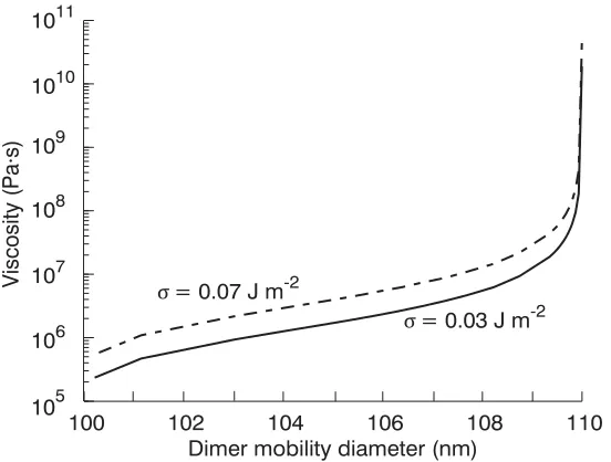
Figure 1 Modeled viscosity as a function of dimer diameter for Dmono = 80 nm,
Duc =110 nm, Dc = 100 nm, and t = 5 s, values characteristic of some
experiments presented in this work. Two surface tensions are depicted, one characteristic of pure organics (0.03 J m-2), one characteristic of a fully
deliquesced particle (0.07 J m-2) ... 119
Figure 2 Schematic of the experimental system including typical flow rates in units of L min-1. The setup differed slightly for the sucrose melting experiment as a
condensation particle counter was utilized to monitor particle generation
xii measurements of coagulated dimers for nominal 80 nm ammonium sulfate
(a) and 50 nm sucrose (b) monomers (solid lines) with associated 95%
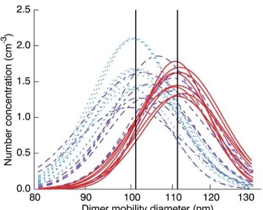
observational prediction intervals (dashed lines) ... 121 Figure 4 Fitted one-mode lognormal curves for all SMPS scans comprising a cooling-
cycle experiment for nominal 80 nm sucrose monomers. Curves are coded according to the RH value of the particular SMPS scan: <48.4% (solid), 48.4%–68.4% (dashed), and >68.4% (dotted). These thresholds were selected so as to depict the relation of each scan to the fitted RHr value of 58.4% ±
0.9% and corresponding expected coalescence states (i.e., uncoalesced, partially coalesced, or fully coalesced). The left and right vertical lines correspond to fitted Dc (101.1 nm ± 0.6 nm) and Duc (111.3 nm ± 0.7 nm)
values, respectively ... 122 Figure 5 Measured dimer mobility diameters for nominal 80 nm adipic acid (a) and
calcium nitrate (b) monomers versus relative humidity with lines indicating fully uncoalesced (top dashed lines) and fully coalesced (bottom dashed lines) diameters as predicted from calibration data ... 123 Figure 6 (a) Measured dimer mobility diameters for nominal 80 nm sucrose monomers
versus relative humidity, fitted lognormal curve (solid line) with associated 95% observational prediction interval (dashed lines), and viscosity estimates for selected diameters in the transition regime assuming a surface tension of 0.03 J m-2. (b) Comparison of sucrose humidity-dependent viscosity estimates
from (a) (line) to measurements reported by Power et al. (2013) (filled circles). The dashed portion of the line indicates onset of coalescence and corresponds to diameters shifts that are within the measurement uncertainty for individual data points. Measurements in panel (a) were collected at temperatures between -3 and -11 °C, whereas the Power et al. (2013) measurements were collected at room temperature ... 124 Figure 7 Measured dimer mobility diameters for nominal 50 nm sucrose aerosol
monomers versus temperature, fitted lognormal curve (solid line) with associated 95% observational prediction interval (dashed lines), and
viscosity estimates for selected diameters in the transition regime assuming a surface tension of 0.03 J m-2 ... 126
Chapter 4
Figure 1 Simplified schematic of the experimental viscosity assessment method
utilized in this work ... 171 Figure 2 Measurements of dimer mobility diameter versus either relative humidity or
xiii (RHr = 44.3% ± 0.9%, Duc = 110.6 nm ± 0.5 nm, Dc = 102.9 nm ± 0.7 nm,
k = 0.9376); (b) sucrose–SDS isothermal humidification at 7 °C (RHr =
43.2% ± 2.9%, Duc = 104.3 nm ± 0.7 nm, Dc = 100.1 nm ± 0.6 nm, k =
0.4056); (c) sucrose–sucrose heating cycle (Tr = 82.8 °C ± 0.7 °C, RHr =
0.9%, Duc = 108.8 nm ± 0.5 nm, Dc = 99.6 nm ± 0.6 nm, k = 0.5626) ... 172
Figure 3 Fitted VFT curve (black curve) for data derived from our heating cycle experiments along with a mean value for the dry glass transition temperature of sucrose from literature. Error bars associated with the glass transition point correspond to one standard deviation of the literature values utilized. Black dashed curves correspond to the 95% observational prediction interval of the fitted VFT equation ... 173 Figure 4 Fitted Gordon–Taylor curve for sucrose (black curve) along with literature
data utilized in its derivation ... 174 Figure 5 Amorphous phase diagram of sucrose aerosol. The diagram shows viscosity
as a function of temperature and relative humidity, along with relevant literature data. Grey curves are lines of constant viscosity. The red dashed line represents a constant viscosity of 5 x 10⁶ Paꞏs. The cyan solid line
represents the glass transition viscosity (1012 Paꞏs). Blue-grey curves are
lines of constant supersaturation with respect to ice ... 175 Figure 6 Modelled sucrose viscosity (black curve) as a function of relative humidity at
T ≈ 22 °C, along with relevant literature data ... 176 Figure 7 Variation in modelled sucrose viscosity with variation in various model
parameters. Red points: viscosity data from Table 1. Purple points and lines: ice nucleation data and supersaturation with respect to ice as in Fig. 5. Dashed grey curves: variation in prediction of 5 x 10⁶ Paꞏs viscosity by our model with
(a) dry glass transition temperature; (b) kGT; (c) κm. Red lines: (a) Tg = 341 K,
the value used in our model; (b) kGT = 5.25, the value used in our model; (c)
κm = 0.14, a value fitted to output from the activity model of eqn (10) at a
temperature of 0 °C and RH between 40% and 50%. Black lines: (a) the lowest and highest reported dry glass transition temperatures for sucrose; (b) kGT = 2.5, a typical value recommended by Koop et al. (c) κm = 0.006, a value
characteristic of non-hygroscopic organics ... 177 Figure 8 Filled contours show observed joint frequency distribution of T and RH
derived from global NCEP reanalysis 4-times daily pressure (p) level resolved dataset for 2015 at p = 500 mb and 300 mb level. Red lines, top to bottom, are modelled η =5 x1 06 Paꞏs isopleths for sucrose assuming κm =
0.01, 0.14, and 0.7, respectively. The black line corresponds to η = 1012 Paꞏs
(glass) for a hypothetical compound with Tg =0 °C and κm = 0.01. States
xiv do not ... 178 Chapter 5
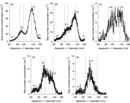
Figure 1 Left: schematic steps used for dimer synthesis. The neutralizer imparts an equilibrium charge distribution. Right: dashed black line corresponds to a theoretical model of the size distribution (a) at the entrance of the coagulation chamber, (b) after exiting the electrostatic filter, and (c) the measured
apparent size distribution with the particle counter after DMA3. Colored lines
indicate various contributions to the signal described in the text. The number #1-#4 in panel (c) indicate four apparent modes in the total size distribution ... 215 Figure 2 Example DTDMA size distributions spectra showing different arrangements
of peaks observed for Dmono = 100 nm. Apparent modes are labeled per the
conventions in Fig. 1. Vertical lines are at 88 nm, 100 nm, and 133 nm, estimated locations for +2-charged dimers, +1-charged decharged monomers, and +1-charged dimers, respectively. Note that the selected mobility diameter scan range mostly elides the peak corresponding to dimers formed from monomers that were doubly charged during size selection, so dimer in this
context refers specifically to +1/-1 dimers ... 216 Figure 3 Example DeTDMA spectrum for myrcene SOA (Dmono = 100 nm) as
transmitted by the negative polarity mobility-selecting DMA at a 2:1 flow ratio. The solid curve is a fit of the data points to a one-mode lognormal equation. The decharged monomer contribution to a full DTDMA SMPS
spectrum under these conditions will be approximately twice this magnitude ... 217 Figure 4 Observed DTDMA SMPS spectra, fitted two-mode lognormal curves, full
simulated DTDMA SMPS spectra, and simulated DTDMA SMPS spectral components for upstream source distributions with lognormal parameters (a) Nup = 3.07 x 106 cm-3, Dup = 61.53 nm, and σup = 1.92 and (b) Nup =
9.06 x 105 cm-3, Dup = 46.14 nm, and σup = 1.69. In both examples Dmono =
80 nm, the flow ratio is 2:1, and the model calculated spectral contributions
of +2/-2 dimers are not significant ... 218 Figure 5 Dependence of Peak #2 magnitude on (a) N and (b) teff along with simulated
model trends assuming an upstream source distribution with Dup = 100 nm, and σup = 1.6. Open circles correspond to data points that deviate from modeled behavior attributed to flow irregularities at low sample flow/high
coagulation time and have been omitted from analysis ... 219 Figure 6 (a) Fitted one-mode lognormal curves for DeTDMA spectra of 100 nm
xv monomer α-pinene SOA where the coagulation chamber was protected by
various amounts of lead brick shielding. In the partial shielding case, bricks were positioned below and to the side of the chamber, whereas in the full shielding cases 1 or more layers of bricks were positioned above the chamber in addition to those below and to the side ... 220 Figure 7 Mean DeTDMA peak heights versus coagulation chamber residence time for
100 nm monomer α-pinene SOA under both shielded and unshielded
coagulation chamber setups, along with associated linear regression lines and model-inferred trend lines. Open markers correspond to experimental
data points that deviate from trend attributed to flow irregularities at low
sample flow/high coagulation time and have been omitted from analysis ... 221 Figure 8 (a) Ratio of modeled DTDMA Peak #2 and Peak #3a as a function of N
under various assumptions of βD for Dmono = 100 nm, assumed Dup = Dmono, assumed σup = 1.6, and a flow ratio of 3:1 (solid lines), along with measured experimental apparent Peak #2/Peak #3 ratios for α-pinene SOA. Dashed horizontal line corresponds to the expected Peak #2/Peak #3b ratio of 4.37 in the absence of decharging per the bipolar charging parameterization of Wiedensohler (1988). (b) Ratios of modelled Peak #2 and Peak #3a magnitudes under two different assumptions of βD, along with the ratio of Peak #1 and Peak #2, all as functions of Dup, for Dmono = 100 nm and a flow ratio of 3:1. In both panels the shaded area corresponds to a
Peak #2/Peak #3a ratio of less than 1.5, an estimate of the minimum necessary for resolution of Peak #2. In panel (b), the assumed upstream size distribution has lognormal parameters Nup = 2 x 106 cm-3 and σup = 1.6 ... 222
Figure 9 (a) Standard deviation in fitted DTDMA Peak #2 mobility diameter for
α-pinene SOA for the indicated mobility-selected number concentrations under different flow ratios in the mobility-selecting DMAs. (b) Simulated DTDMA SMPS spectra for 80 nm monomers assuming βD = 2.0 x 10⁻⁵ s-1 and
an upstream source with lognormal distribution Nup = 9.06 x 105 cm-3,
Dup = 46.14 nm, and σup = 1.69 under different assumptions of flow ratio
(contour labels) ... 223 Figure 10 (a) Model calculated height of the primary dimer peak at different Dmono
assuming teff = 60 s, a flow ratio of 3:1, and an upstream lognormal
distribution with Nup = 2 x 106 cm-3, 1.5 x 106 cm-3, or 1.2 x 106 cm-3;
σup = 1.6; Dup = Dmono. Shaded area corresponds to peak heights less than
5 cm-3, a coarse estimate of minimum peak height for reliable peak fitting in
prior work in the presence of moderate decharging. (b) Model calculated required Nup for a mobility-selected number concentration of 100,000 cm-3
at different mobility-selected diameters assuming an upstream lognormal distribution with σup = 1.6 and Dup = Dmono. In both panels, curves are fits of
the plotted data to power equations of the form y = axb + c and are provided
xvi Figure 11 Variations in apparent +1 mobility diameter with thermal conditioning
for DCIC dimers formed via coagulation of monomers of α-pinene SOA from a stream of the specified number concentrations onto monomers of (a) α-pinene SOA from a stream of number concentration of
290,000±10,000 cm-3 (b) PolyWax 850 monomers from a stream of
number concentration of 170,000±20,000 cm-3. Dashed horizontal lines
represent approximate values of Duc and Dc. Error bars have been elided
from the lowest analyte concentration cases in each panel for clarity ... 225 Figure 12 Predicted mobility diameter shifts between Duc and Dc using the model
of Gopalakrishnan et al. (2015a) for cylindrical rod, doublet of spheres, or prolate spheroid geometries to predict Duc and assuming Dc is equal
to the diameter of the volume-equivalent sphere, overlaid with available experimental data. The predicted diameter shift assuming Duc is 1.1x larger
than Dc is also shown. The shaded area corresponds to y-axis values of 3 nm
or less. Some experimental data points with nominal apparent monomer
diameters of 80 or 100 nm have been jittered ±2 nm for purposes of clarity... 226 Chapter 6
Figure 1 Condensation profile (radius vs time) for an aqueous glucose droplet (20 °C, RH transition of 25−79%): measurement (gray points) and fitted mKWW equation (black curve). The vertical gray dashed line represents
τ = 3.6 s ... 248 Figure 2 (a) RH-dependent viscosities of raffinose, trehalose, sucrose, glucose,
sodium nitrate, and PEG4, with polynomial equations from Song et al. for the saccharides and Baldelli et al. for sodium nitrate (solid lines). (b) Experimental RH-dependent glass transition temperatures for binary aqueous solutions of raffinose (yellow squares and circles), sucrose (red triangles, left triangles, right triangles, and upside down triangles), and sodium nitrate (blue squares). Pure component glass transition temperatures (diamonds) for raffinose, sucrose, sodium nitrate, and water are also reported. Fits to the Gordon−Taylor equation using literature parameters for raffinose and sucrose are indicated by solid lines ... 249 Figure 3 Fitted experimental characteristic condensation times versus the (a) final RH,
(b) estimated initial viscosity of the droplet prior to the condensation step, the (c) temperature of the condensation measurement. Dashed gray horizontal lines delineate the 1 order of magnitude range in τ containing most
experimental values. The legend is at top for (a−c) ... 251 Figure 4 Comparison of fitted experimental and modeled characteristic time scales
using the Kulmala equation and mKWW fitting for the experiments
xvii Appendix A
Figure S1 Influence of (a) branching and (b) OH-group position on mean literature glass transition temperature for species containing 1-3 hydroxyl groups. Note triols are elided from (b) because all such compounds with available data
have both terminal and internal OH groups ... 337
Figure S2 Mean literature glass transition temperatures for compounds containing 1 or 2 OH groups versus the length of the compound’s backbone carbon chain ... 338
Appendix B Figure S1 Dimer geometry assumed in the derivation of the relationship between the degree of dimer coalescence and particle viscosity ... 391
Figure S2 Sodium dodecyl sulfate ... 393
Figure S3 PEG-1000 ... 394
Figure S4 PEG-10000 ... 395
Figure S5 Ammonium sulfate ... 396
Figure S6 Monosodium α-ketoglutaric acid ... 397
Figure S7 Sodium chloride ... 398
Appendix C Figure S1 Plot depicting how the relative humidity where viscosity equals 5 x 10⁶ Paꞏs (open red circle) was interpolated from data digitized from Power et al. (solid red circles). Solid black line: fitted linear regression line; dotted black lines: 95% confidence interval of the fitted regression line; dashed black lines: 95% observational prediction interval of the fitted regression line ... 401
Figure S2 Variation in placement of modelled 5 x 10⁶ Paꞏs and 1012 Paꞏs isopleths where the relationship between sucrose mass fraction and water activity was modelled using either the approach of Zobrist et al or a mass-based hygroscopicity parameter approach with a fixed parameter value of 0.14, characteristic of sucrose ... 402
xviii Figure S4 Measurements of dimer mobility diameter versus RH for the sucrose-sucrose
isothermal humidification experiment performed at T = 5 °C, including fitted logistic curve (solid black curve) and 95% observational prediction interval (dashed black curves). (RHr = 45.5% ± 0.1% Duc = 109.0 nm ±
0.8 nm, Dc = 103.0 nm ± 0.7 nm, k = 9.525) ... 404
Figure S5 Measurements of dimer mobility diameter versus RH for the sucrose-sucrose isothermal humidification experiment performed at T = 12 °C, including fitted logistic curve (solid black curve) and 95% observational prediction interval (dashed black curves). (RHr = 43.2% ± 1.5%, Duc = 109.4 nm ±
0.7 nm, Dc = 102.4 nm ± 1.3 nm, k = 0.5982) ... 405
Figure S6 Measurements of dimer mobility diameter versus RH for the sucrose-sucrose isothermal humidification experiment performed at T = 15 °C, including fitted logistic curve (solid black curve) and 95% observational prediction interval (dashed black curves). (RHr = 40.7% ± 1.0%, Duc = 108.9 nm ±
0.8 nm, Dc = 101.5 nm ± 0.9 nm, k = 0.8967) ... 406
Figure S7 Measurements of dimer mobility diameter versus RH for the sucrose-sucrose cooling cycle experiment performed new for this work, including fitted logistic curve (solid black curve) and 95% observational prediction interval (dashed black curves). (RHr = 46.8% ± 1.2%, Tr = 0.1 °C ± 1.2 °C, Duc =
109.2 nm ± 0.8 nm, Dc = 102.7 ± 0.8 nm, k = 1.222) ... 407
Figure S8 Measurements of dimer mobility diameter versus RH for the first sucrose- SDS cooling cycle experiment referenced in Table 1 of the manuscript, including fitted logistic curve (solid black curve) and 95% observational prediction interval (dashed black curves). (RHr = 48.6% ± 3.1%, Tr =
-1.3 °C ± 1.1 °C, Duc = 104.4 nm ± 0.7 nm, Dc = 100.6 nm ± 0.9 nm,
k = 0.3698) ... 408 Figure S9 Measurements of dimer mobility diameter versus RH for the second sucrose-
SDS cooling cycle experiment referenced in Table 1 of the manuscript, Including fitted logistic curve (solid black curve) and 95% observational Prediction interval (dashed black curves). (RHr = 48.9% ± 3.5%, Tr = -3.4 °C,
Duc = 106.8 nm ± 0.5 nm, Dc = 102.3 nm ± 0.6 nm, k = 1.697) ... 409
Figure S10 Measurements of dimer mobility diameter versus temperature for the first sucrose-sucrose heating cycle referenced in Table 1 of the manuscript, including fitted logistic curve (solid black curve) and 95% observational prediction interval (dashed black curves). (Tr = 83.1 °C ± 0.6 °C), RHr =
0.8% ± 0.1%, Duc = 108.4 nm ± 0.3 nm, Dc = 98.1 nm ± 0.5 nm, k = 0.4646) ... 410
xix observational (dashed black curves). (Tr = 83.2 °C ± 0.7 °C, RHr = 0.8% ±
0.1%, Duc = 107.9 nm ± 0.5 nm, Dc = 98.5 nm ± 0.5 nm, k = 0.5814) ... 411
Figure S12 Fitted VFT curve as derived for sucrose when fixing the A parameter to a value of -5. The curve fit utilized both viscosity data derived from heating cycle experiments and mean literature Tg. Error bars associated with the
glass transition point corresponds to one standard deviation of the literature values utilized. Black dashed curves correspond to 95% observational
prediction intervals of the fitted VFT equation ... 412 Figure S13 Fitted VFT as derived for sucrose utilizing only data from heating cycle
experiments and not considering mean literature Tg. Error bars associated
with the glass transition point correspond to one standard deviation of literature values utilized. Black dashed curves correspond to the 95%
observational prediction interval of the fitted VFT equation ... 413 Figure S14 Variation in placement of modelled 5 x 10⁶ Paꞏs and 1012 Paꞏs isopleths
where dry sucrose glass transition temperature was determined either using a literature value or an extrapolation of our own dry sucrose viscosity
measurements ... 414 Appendix D
Figure S1 Simplified flow schematic for the coagulation chamber assembly subsystem, including flow rates for an idealized experiment with two 0.3 L coagulation chambers installed, 1.1 L min-1 sample flow through
both mobility-selecting DMAs (a typical value) and a coagulation chamber residence time of 30 s. The schematic above includes the 0.3 L mixing volume used in experiments probing coagulation time effects. Accordingly, the effective coagulation time for the setup presented is 42 s, including the estimated 6 s of dwell time outside of the mixing volume and coagulation chambers. The amount of flow to exhaust is directly regulated
by the needle valve. ... 419 Figure S2 Photograph showing the lead brick shielding used to encase the coagulation
chamber ... 420 Figure S3 Photograph showing the lead brick shielding used to encase the coagulation
chamber with the top layers removed ... 421 Figure S4 Photograph showing position of the utilized Cs-137 radiation source relative
to the coagulation chamber during the radiation sensitivity experiment ... 422 Appendix E
xx equations (black curves) and simulated growth curves (red curves) for
representative (a) sodium nitrate and (b) sucrose droplet condensation experiments at 0 °C. The dashed red curves represent uncertainty in the simulated growth curves arising due to an assumed uncertainty of ±0.1 µm (ie. the uncertainty of the geometric optics sizing procedure) on the initial droplet radii. The dashed vertical lines are positioned at the fitted
experimental characteristic times ... 457 Figure S2 Comparison of the radius dependence of the modelled bulk mixing time in
10 % RH increments (grey solid lines) and 25% and 78% RH (black solid lines) with modelled condensational growth timescales for sucrose particles at 20 °C and for an RH step from 25% to 78% (red circles). The mean experimental timescale for a sucrose particle (~8 μm) ~25 – 75 % RH step at 20 °C is indicated by the red square ... 458 Figure S3 Modeled growth curves under various assumptions of mass accommodation
coefficient (α) for the representative sucrose condensation experiment (grey data points) from Fig. S1b. Thin dotted red curves correspond to modelled growth curves assuming logarithmically spaced values of the mass
1 CHAPTER 1
2 Atmospheric aerosol is central to various processes of meteorological or climatological concern (McNeill 2017; Fan et al. 2016; Boucher et al. 2013) and is a pollutant of significant concern for human health (Shiraiwa et al. 2017b). Much of the particulate matter in the
atmosphere is comprised of organic compounds (Volkamer et al. 2006), and this organic aerosol (OA) fraction consists of thousands of distinct compounds (Goldstein and Galbally 2007). Broadly, atmospheric OA can be separated into two classes: primary (POA) and secondary (SOA). POA is directly emitted in the particulate phase, such as combustion products (Tsimpidi et al. 2016; Presto et al. 2012) and aerosolized bioaerosols (Després et al. 2012). In contrast, SOA precursors are emitted in the gas phase, such as isoprene and its derivatives from biogenic sources (Shrivastava et al. 2017a; Jokinen et al. 2015; Wyche et al. 2014; Fu et al. 2014) or aromatics from anthropogenic sources (Jathar et al. 2013; Gentner et al. 2012; Pandis et al. 1992). These precursors subsequently undergo oxidation reactions producing progressively less volatile products (Ziemann and Atkinson 2012; Kroll et al. 2011; Jimenez et al. 2009).
Eventually, equilibrium vapor pressure is sufficiently reduced that some fraction of these
3 The difference in viscosity between a liquid such as water and an amorphous solid
(glassy) phase is approximately 15 orders of magnitude (Shiraiwa et al. 2011). POA can be highly viscous. Long-chain hydrocarbons typical of anthropogenic emissions may be solid at near-ambient and colder temperatures (Shrivastava et al. 2017b), and glassy particles comprised of soil material aerosolized via surface impacts of precipitation droplets have been observed (Wang et al. 2016). Until recently, it has been thought that SOA was primarily liquid. In a theoretical treatment, Marcolli et al. (2004) argued that the liquid phase was thermodynamically preferred. Experimentally, observed trends in both deliquescence relative humidity (Marcolli et al. 2004) and evaporation behavior (Cappa et al. 2008) for carboxylic acids argued for
increasingly liquid-like behavior in organic mixtures with additional components. Given that the mixtures in the studied works had a comparatively small number of constituents relative to atmospheric OA, expecting such OA to be liquid in practice was a reasonable extrapolation. The existence of atmospheric SOA in highly viscous forms was postulated by Zobrist et al. (2008), who observed that a number of common aqueous OA proxy systems, including several multi-component mixtures, underwent a glass transition at temperatures of atmospheric relevance. This was confirmed by Virtanen et al. (2010), who observed amorphous solid particles in electron micrographs of SOA derived from boreal forest emissions. More recently, global modelling by Shiraiwa et al. (2017a) suggests that environmental conditions favorable for SOA to exist in a glassy phase become increasingly common with altitude, and that in the upper troposphere SOA may be predominately glassy. Semi-solid viscosities have been directly measured in dry,
4 cannot necessarily be assumed in numerical treatments of chemical, microphysical, or radiative interactions. Accordingly, there is scientific merit in quantifying OA viscosity and characterizing the processes that drive it and are modulated by it.
OA viscosity is, however, a very broad research topic. It touches on organic, physical, and analytical chemistry; cloud microphysics; and aerosol mechanics. Full understanding will require development of new instrumental methods and robust numerical models. As direct measurement of ambient OA is often not feasible, suitable proxy and laboratory-generated SOA systems must be identified and characterized. Thus, there are many aspects for research, although a full treatment of OA viscosity is well beyond the scope of a single Ph.D. dissertation. The remainder of this chapter will discuss the existing state of knowledge regarding OA viscosity, with an emphasis on the facets of this broad problem that directly motivated the research in the chapters to follow. These subsequent chapters are then briefly introduced at the end of the literature survey.
Possible Implications of Viscous Organic Aerosol
It is worth considering why variations in viscosity observed across OA are of potential scientific interest. A conventional value of 1012 Paꞏs is typically assumed for glassy aerosol
(Debenedetti and Stillinger 2001). By comparison, liquid water has a viscosity of 0.0089 Paꞏs at 25 °C (Kestin et al. 1978), implying observed viscosity in atmospheric aerosol may span more than fifteen orders of magnitude. Per the Stokes-Einstein (SE) relationship (Shiraiwa et al. 2011), diffusivity of small molecules within an aerosol matrix is inversely proportional to the particle viscosity (η):
𝐷 𝑘 𝑇
5 where kB is Boltzmann’s constant, T is the absolute temperature, and a is the molecular radius. It is established that the SE relationship does not strictly hold, even at relatively low viscosities (Marshall et al. 2016). However, it is not unreasonable to expect that the difference in diffusivity between a particle with water-like viscosity and one with glass-like viscosity is still many orders of magnitude, particularly for relatively large molecules. Even for particles in the semi-solid regime (102 < η < 1012 Paꞏs) (Shiraiwa et al. 2011), diffusivity may be reduced by multiple
orders of magnitude relative to a liquid phase. Deviations from SE behavior can be accounted for through the use of fractional SE relationships, where viscosity and diffusivity are related via an empirically derived power (ξ). At constant temperature, such an equation has the following form:
𝐷 𝐶𝜂 , (2)
where C accounts for the non-viscosity terms on the right side of Eq. (1). For water in sucrose at 296 K, a value for ξ of 0.57 has been proposed (Price et al. 2016), implying an approximately half order of magnitude decrease in diffusivity for each order of magnitude increase in viscosity. Characteristic mixing time (τ) within a particle of diameter Dp is inversely related to the
diffusivity (Seinfeld and Pandis 2006):
𝜏 𝐷
4𝜋 𝐷. (3)
As such, if viscous inhibitions are present, particles may equilibrate on timescales longer than those of most processes in the atmosphere (Maclean et al. 2017). Possible implications of such inhibitions are considered next.
6 diffusional flux and slowing particle growth. If growth is slowed sufficiently relative to
timescales of atmospheric processes such as adiabatic cooling in an updraft, actual droplet size distributions will differ from the predictions of purely equilibrium models such as Köhler (1936) theory. Inhibited hygroscopic growth of viscous aerosol has been observed at low (<45%) RH (Bones et al. 2012; Tong et al. 2011). However, growth kinetics at higher RH are of greater relevance to cloud processes, and by extension, cloud radiative effects. Modelling studies suggest that diffusional inhibitions may be of less concern at high RH (O’Meara et al. 2016; Lienhard et al. 2015), perhaps due to plasticization from water uptake removing diffusional inhibitions (Pajunoja et al. 2015). However, direct measurements comparing timescales of condensational growth to initial particle viscosity at high RH have not been previously reported. This is investigated further in Chapter 6 of this work.
Diffusional inhibitions may also influence the kinetics of particle-phase chemical
7 anthropogenic pollutants to previously pristine regions (Shrivastava et al. 2017b; Zelenyuk et al. 2012). Recently, Liu et al. (2018) have observed that brown carbon forms more readily from initially non-absorbing SOA at 60% RH than at 20% RH, environmental conditions consistent with lower particle viscosity and higher diffusivity with the particle matrix. Chim et al. (2017) found that uptake of OH radicals by aqueous droplets of 2-methylglutaric acid increased with increasing RH and argued that this was more likely due to changes in bulk viscosity than changes in reaction mechanism arising from increased particle water content. Similar observations of RH-dependent kinetics have been made for the ozonolysis of shikimic acid (Steimer et al. 2015), uptake of ammonia by α-pinene SOA (Kuwata and Martin 2012) and uptake of both OH (Davies and Wilson 2015) and N2O5 (Gržinić et al. 2015) by citric acid aerosol.
Finally, viscous organic aerosol may modulate ice nucleation pathways, with possible implications for cirrus cloud formation. The latter possibility is of potential concern to global climate models, as cirrus layers influence the global radiative balance (Campbell et al. 2016; Lee et al. 2009). Murray (2008) observed that citric acid solutions could become glassy at conditions similar to the tropical tropopause, and that in such solutions ice crystallization was inhibited. This was extended in subsequent works, where heterogenous ice nucleation was observed on glassy particles in a cloud simulation chamber for first citric acid aerosol (Murray et al., 2010) and then various other OA proxies (Wilson et al. 2012). Elsewhere, Wang et al. (2012) observed heterogeneous ice nucleation onto naphthalene SOA and Ignatius et al. (2016) observed
8 via semi-solid aerosol may predominate. If OA viscosity is an important consideration for
treatments of ice nucleation, it should be noted that relevant viscosities are currently not well constrained. Glassy (1012 Paꞏs) viscosities may not be necessary for depositional mode freezing,
for example. In practice, required viscosities for heterogeneous nucleation may be quite low. For example, contact mode nucleation (Vali et al. 2015) facilitated by hydrocarbons with viscosities below 1 Paꞏs has been observed (Collier and Brooks 2016).
Organic Aerosol Formation and Ageing
Before considering methods of quantifying OA viscosity, it is worth briefly discussing the chemistry of OA, in order to emphasize to the reader that many factors influence OA
9 Soil organic material (SOM) dissolved in a surface water layer is entrained into air bubbles formed from impact of precipitation droplets. These bubbles subsequently burst, aerosolizing the SOM, which quickly becomes viscous due to drying. Finally, bioaerosols such as pollen and microbes also contribute to the POA fraction (Fröhlich-Nowoisky et al. 2016; Després et al. 2012).
SOA formation mechanisms are exceptionally complex and have been the subject of several review articles (Ziemann and Atkinson 2012; Carlton et al. 2009; Hallquist et al. 2009; Kroll and Seinfeld 2008). Accordingly, only a high-level discussion of SOA formation will be presented in the following paragraphs, and the reader is directed to the referenced review articles and citations therein for additional details. SOA precursors are comprised of a variety of
anthropogenic and biogenic emissions. Broadly speaking, these gases (VOCs) are (typically unsaturated) hydrocarbons with limited oxidation. In unpolluted environments, isoprene and its derivatives, particularly monoterpenes and sesquiterpenes, dominate (Shrivastava et al. 2017a). In urban regimes, various alkanes, alkenes, and aromatic hydrocarbons can act as SOA
precursors (Gentner et al. 2017; Hildebrandt et al. 2009; Ng et al. 2007). Slightly more
complicated precursors include fatty acids from meat cooking (Rogge et al. 1991) and products of biomass burning (Kelly et al. 2018; Bian et al. 2017). Molecular oxygen (O2) is the most
prevalent oxidizer in the atmosphere by a large margin. However, direct reaction between O2 and
common VOCs proceeds much too slowly to be of atmospheric relevance (Seinfeld and Pandis 2006). Accordingly, SOA formation is driven by radical chemistry. Four radical species are of particular importance: hydroxyl radical (OH), nitrate radical (NO3), ozone (O3), and atomic
chlorine (Cl) (Ziemann and Atkinson 2012). NO3 is primarily relevant to nighttime chemistry as
10 between VOCs and OH, NO3, and Cl typically form either an alkyl radical via abstraction of a
hydrogen atom from a C-H bond by the oxidant or a substituted alkyl radical via direct addition of the oxidant to a carbon-carbon double bond (Ziemann and Atkinson 2012). O3 attacks
carbon-carbon double bonds, forming a ring-shaped intermediate product known as a Criegee
intermediate that subsequently decays to an alkyl radical and a free OH radical (Ziemann and Atkinson 2012).
Regardless of formation mechanism, the primary reaction pathway for these alkyl-type radicals is addition of molecular oxygen to form peroxy radicals (RO2ꞏ). Through subsequent
reactions, these peroxy radicals can form alcohols (ROH), carboxylic acids (RC(O)OH), carbonyls (RC(O)R’), hydroperoxides (ROOH), and peroxy acids (RC(O)OOH), as well as organic nitrates (RON2) and peroxynitrates (ROON2) in the presence of NOx (Ziemann and
Atkinson 2012). The addition of oxygenated groups tends decrease equilibrium vapor pressure (Goldstein and Galbally 2007). Progressive oxidation is characteristic of organic species evolution in the atmosphere (Kroll et al. 2011; Jimenez et al. 2009), and after sufficient
oxidation, vapor pressure will be reduced sufficiently as to allow some fraction of the chemical species to partition into the particulate phase. The viscosity of the resulting particles will in part depend upon the number and type of functional groups added; this relationship is investigated further in Chapter 2 of this work. Quantification of gas-particle partitioning along with potential implications of partitioning on viscosity are considered next.
11 product with a low equilibrium vapor pressure (C1*) and a product with a high equilibrium vapor pressure (C2*). Assuming the two products have individual molar yields (ratio of moles produced to moles of total gases reacted) a1 and a2 respectively, this can be represented by the following equation (Odum et al. 1996):
𝑌 𝐶 𝑎
𝐶 𝐶∗
𝑎
𝐶 𝐶∗ (4)
Two-product-style approaches for modelling partitioning can be extended to an arbitrary number of bins. One common method is the volatility basis set (VBS) (Donahue et al. 2006). In this approach, similar to the Odum et al. (1996) method, bins are defined by effective vapor-phase saturation concentrations (C*i), here typically defined as logarithmically spaced powers of 10. Knowing the total concentration of organic mass in the particulate phase (COA), the fraction of each bin in the aerosol phase (ξi) can be calculated by solving iteratively the below equations:
𝜉 1 𝐶
∗
𝐶 (5a)
𝐶 𝜉 𝐶 (5b)
where Ci is the total organic mass concentration in either phase for each bin. From the above, it is clear that at higher values of COA, a higher fraction of more volatile constituents will partition into the particulate phase. This may have implication for the viscosity of the resulting aerosol. An approximately inverse relationship between viscosity and equilibrium vapor pressure has been noted in bulk organic samples (Thomas et al. 1979; Sastri and Ramana Rao 1970; Mitra 1954). This suggests that if a larger fraction of highly volatile constituents are present in the aerosol phase, particle viscosity will be smaller than if those highly volatile constituents
12 systems present, but their respective concentrations as well. This is consistent with observations by Grayson et al. (2016), who noted that the viscosity of α-pinene SOA decreased by
approximately 1.5 orders of magnitude as the aerosol mass loading increased 2 orders of magnitude from 100 to 10,000 µg m-3.
Regardless, from the above discussion, it should be apparent that OA is an exceptionally complex system. The large number of potential product species implies that isolation of specific OA constituents in suitable quantity for viscosity analysis will be difficult at best. Accordingly, classic industrial rheological approaches may scale poorly to the OA domain, and specialized methodologies for quantifying and representing OA viscosity may be necessary. Previously existing work on those latter two topics will be discussed in the next two sections.
Measuring Aerosol Viscosity
In discussing methods for measuring OA viscosity, we shall first consider the special case of the viscosity associated with transition between an amorphous solid (glassy) phase and an amorphous semi-solid phase, conventionally 1012 Paꞏs (Debenedetti and Stillinger 2001). The
13 As for directly measuring viscosity itself, common methods for analyzing large, bulk samples can be suitable to readily available organic proxy systems such as carbohydrates and common organic food acids, but are poorly suited to SOA. As discussed in the preceding section, SOA formation is exceptionally complex, with highly branched reaction mechanisms and various sensitivities to environmental conditions. Measuring distinct viscosity profiles for these
individual constituents is highly impractical. Many of these constituents are not commercially available, and the frequent occurrence of highly reactive (and in bulk, potentially explosive) peroxy groups limits the degree to which such compounds can be synthesized and isolated in quantities suitable for bulk analysis. Even when SOA products are analyzed as a complete mixture, bulk methods will generally be inadequate. Bulk rheological methods exist for microliter volumes, but are typically limited to very low viscosities (Renbaum-Wolff et al. 2013b). When only micrograms of material can be collected, methods suitable for nanoliter volumes are required. Thus, the need for aerosol-specific methodologies for measuring viscosity should be apparent.
A broad class of such techniques involves observations of various relaxation processes in supermicron-sized particles via optical imaging. One such example is the bead-mobility method, first introduced by Renbaum-Wolff et al. (2013b). A supermicron (30 µm – 50 µm diameter) droplet of the material under study is placed on a slide. Next, ~1 µm beads of melamine or a similar hydrophilic compound are nebulized over the droplet; several of these are subsequently incorporated into the droplet. The slide is then positioned in a temperature- and
humidity-controlled flow cell. Shear stresses between the N2 flow in the cell and the surface of the droplet
14 which in turn can be related back to viscosity through a calibration curve. This method is limited to viscosities where bead speed is fast enough to be measurable. Renbaum-Wolff et al. (2013b) estimates the maximum such viscosity as 103 Paꞏs, which functionally restricts its applicability to
liquids and the low-end of the semi-solid viscosity range. As such, this method is typically used concert with other measurement approaches, frequently including the poke flow technique discussed next (Grayson et al. 2017; M. Song et al. 2016; Renbaum-Wolff et al. 2013a).
The basic idea of poke flow was first introduced for qualitatively differentiating liquids and non-liquids by Murray et al. (2012) and for quantitatively measuring viscosities by
Renbaum-Wolff et al. (2013a), with more thorough validation of the latter subsequently provided by Grayson et al. (2015). As with the bead-mobility method, a supermicron particle is
maintained on a hydrophobic substrate in a temperature- and humidity-controlled flow cell. A sharp needle is inserted through a hole in the flow cell and pokes the previously spherical particle, forcing it into a torus shape. Relaxation of the particle from a torus back to a sphere is then observed via optical imaging. These observations are used to calculate a characteristic relaxation time, which is then related to viscosity by use of numerical flow simulations.
Recently, Lee et al. (2017) have proposed that transitions between glassy solid and semi-solid phases and between semi-semi-solid and liquid phases can be detected using atomic force microscopy. In the former case, the transition is detected by the presence of a viscoelastic response, while in the latter case it is delineated by the ratio of probe penetration distance to particle height reaching a steady-state for a given force. For aqueous sucrose particles, these transitions were observed at RH values corresponding to viscosities 1011.2 and 102.5 Paꞏs (Lee et
15 common literature conventions of 1012 (Debenedetti and Stillinger 2001) and 102 Paꞏs (Shiraiwa
et al. 2011), respectively.
Yet another approach utilizes molecular rotors. Molecular rotors are molecules with twisted conformations that fluoresce when intramolecular rotation is hindered. The characteristic timespan of this fluorescence is related to the viscosity of the medium (Lee et al. 2018). Variants of this approach have been primarily utilized in rheological studies of living cells (Kubánková et al. 2017; Lee et al. 2016; Haidekker and Theodorakis 2007); however, it has been demonstrated that the basic methodology is applicable to droplets of atmospherically relevant material as well (Hosny et al. 2013).
Finally, one particularly notable droplet method (Power et al. 2013) utilizes optical tweezers (Wills et al. 2009), an instrumental method for trapping and manipulating particles using the radiation pressure produced by a tightly focused laser beam. Using the tweezers, two separate droplets are brought into contact, forming a dimer. Changes in morphology as the dimer relaxes into a sphere are observed using brightfield microscopy. Viscosity is inferred from the timescale required for the dimer to fully coalesce and virtually the entire viscosity range of atmospheric relevance can be probed. To date this technique has been applied to RH-dependent viscosity measurements for a variety of common proxy systems for organic aerosol (Y. Song et al., 2016), aqueous sodium nitrate (Baldelli et al. 2016), aqueous mixtures of sucrose and citric acid (Marsh et al. 2018), and aqueous erythritol (Chu et al. 2018). The idea of relating dimer coalescence to viscosity, first pioneered via this method, is the basis of the instrumental method that will be detailed in Chapters 3 and 5 and utilized in Chapter 4 of this work.
16 this nonetheless translates to particle diameters on the supermicron scale. Much aerosol of
atmospheric interest is of diameters of 100 nm or less (Betha et al. 2013; Aiken et al. 2009; Kannosto et al. 2008; Rupakheti et al. 2007), and scale dependence of aerosol viscosity is currently not well understood. Furthermore, even size-selected atmospheric aerosol may consist of particles of differing chemical composition and mixing state. In such cases effective radiative behavior and other physicochemical properties of the bulk may differ from those of the
individual constituent morphologies. Finally, for products of environmental chamber or flow reactor experiments acquisition of adequate amounts of material for analysis via single-droplet techniques may require the use of filter extracts, which may involve reactions between the collected material and the extraction solvent (Bateman et al. 2008). As such, there is also
motivation for development of rheological techniques for bulk, nanoscale aerosol to complement single-particle methodologies.
One such method exploits a phenomenon known as impactor bounce (Jain and Petrucci 2015; Saukko et al. 2012; Virtanen et al. 2010). This technique is based upon a simple principle: the more solid-like a particle, the greater likelihood that it will fail to adhere to the collection substrate in an impactor. The fraction of particles that bounce as such can be determined by comparing the number of particles actually collected to an expected number derived from concentration measurements of the same input particle stream using a scanning mobility particle sizer (SMPS) (Wang and Flagan 1990). Bounce is an appealing technique because it utilizes ubiquitous aerosol instrumentation and does not require high aerosol number concentration. As such, it can be readily utilized in field deployments in addition to laboratory studies.
17 in liquid phase. For example, bounce measurements have been used by Bateman et al. (2016) to determine that ambient particles in the Amazon rain forest are liquid under most environmental conditions.
Alternatively, there has been interest in methods probing spherical relaxation, essentially bulk aerosol analogues to the droplet-based method of Power et al. (2013) discussed above. Järvinen et al. (2016) used measurements of depolarization of backscattered light to detect when chamber-generated aggregates of α-pinene SOA relaxed to a sphere, noting that such a transition corresponded to an approximate viscosity of 107 Paꞏs. Zhang et al. (2015) considered how the
dynamic shape factor (χ) of dimerized α-pinene SOA varied with viscosity. Dynamic shape factor is a correction to Stokes drag calculations accounting for deviations from the behavior of an equivalent spherical particle due to asphericity. It will have a value of approximately 1.1 for a dimerized particle, decreasing to 1.0 for a coalesced sphere (Hinds 1999). If particle mass (mp) is known, such as measured using Aerosol Particle Mass Analyzer (Ehara et al. 1996), χ can be calculated for mobility-selected particles of mobility diameter Dm via the below equation (Kasper 1982):
𝜒 𝐷
6𝑚 𝜋𝜌⁄ ⁄
𝐶 6𝑚 𝜋𝜌⁄ ⁄
𝐶 𝐷 , (6)
where ρ is an assumed particle density and Cc is a slip correction function. Using numerical simulation, Zhang et al. (2015) estimated that the spherical coalescence process covered viscosities between ~108 Paꞏs and 106 Paꞏs for flow tube-generated α-pinene SOA.
18 example, in the Zhang et al. (2015) work, it was necessary to carefully select the dimer mobility diameter utilized in order to minimize the influence of non-dimer morphologies on subsequent measurements. As such, a method for directly preparing and isolating dimerized particles may be desirable. One potentially useful approach has been demonstrated by Maisels et al. (2000). This method is based upon the following observation: when two oppositely charged monomers coagulate, the resulting dimer will be charge neutral. As such, uncoagulated monomers retain a charge and can subsequently be removed via electrostatic filtration. The streams of oppositely charged particles can be produced by using two differential mobility analyzers (DMAs) (Knutson and Whitby 1975) of opposite polarity. Relatedly, the form of Eq. (6) suggests that if the ratio of the slip correction between spherical and aspherical particles remains approximately constant, the change in shape factor associated with spherical relaxation can be detected simply by comparing measurements of mobility diameter using a SMPS, eliminating the need to measure particle mass. Such an assumption is typically reasonable for particles with diameters on the order of 100 nm (Suda and Petters 2013). These two approaches will be combined in the viscosity method introduced in Chapter 3, applied in Chapter 4, and further characterized in Chapter 5 of this work.
Modelling Aerosol Viscosity
19
𝑉 𝑟 𝐴
𝑟 𝐵
𝑟 (7)
where ALJ and BLJ are constants characteristic of repulsive and attractive interactions,
respectively. Under such a formulation, net attractive forces (represented by a negative value of VLJ) strengthen as intermolecular distance decreases, except at very close distances where repulsive forces increasingly dominate due to quantum mechanical effects. At higher
temperatures, molecules exhibit greater mobility, and thus any two molecules will spend less time in close proximity, resulting in weaker intermolecular attractions and a less viscous liquid overall. In the troposphere, temperatures can range from approximately 190 K at the tropical tropopause (Seidel et al. 2001) to approximately 330 K in the hottest deserts (El Fadli et al. 2013). The effect of such a 140-degree difference in temperature on viscosity can be dramatic. For example, 190 K is below the glass transition temperature (Tg) of 1,2,6-hexanetriol (Nakanishi and Nozaki 2011), a liquid organic used as a SOA proxy (Cai et al. 2015; Zawadowicz et al. 2015), whereas at 330 K its viscosity is on the order of 1 Paꞏs (Meister et al. 1960), at least 11 orders of magnitude smaller.
20 between 15% and 80% RH, ten orders of magnitude for sucrose between 31% and 83% RH, and seven orders of magnitude for citric acid between 4% and 70%. For SOA, differences of
viscosity of approximately six orders of magnitude have been reported for isoprene-derived SOA between 0% and 85% RH (M. Song et al. 2015), approximately seven orders of magnitude for toluene-derived SOA between 30% and 90% RH (M. Song et al., 2016), and five to seven orders of magnitude for α-pinene SOA between 0% and 90% RH (Zhang et al. 2015). Conversely, a particle subject to drying may undergo an RH-induced glass transition (Mikhailov et al. 2009).
At small diameters (< 100 nm) thermodynamic calculations suggest a scale dependence may also be present (Cheng et al. 2015), although to the author’s best knowledge no significant experimental study of this relationship has been published to date, and this variable will not be considered in the discussion below.
Methods of estimating Tg will be considered first. As the glass transition is associated with a change in energy conformation (Angell 1991), it is plausible that glassy solids have distinct properties relevant to aerosol physicochemistry that are lacking even in viscous semi-solids. Regardless, even if the distinction between glassy solid and semi-solid OA is more academic than functionally distinguishing, Tg itself is often an important parameter in more general treatments of viscosity, as will be shown later in this section. A simple parameterization for Tg is the Boyer-Beaman or Boyer-Kauzmann rule (Boyer 1963), which relates Tg to the crystalline melting temperature (Tm) of the solute via a constant scaling factor (g):
𝑇 𝑔𝑇 . (8)