This dissertation is composed of three essays. The purpose of the first essay is to
investigate the effect that higher temperatures have on the size of wildfires in the western
United States controlling for suppression effort, precipitation, and other factors. Using data
for 466 wildfires that occurred on U.S. Forest Service land between 2003 and 2007, I find
that an increase in temperature of 1°C is associated with a 12% increase in wildfire size,
holding all other factors constant. Given that current climate models predict temperatures to
rise by 1.6 to 6.3°C, this estimate suggests mean wildfire size could increase by 20% to 79%.
Off-setting this increase in wildfire size would require an increase in suppression
expenditures of at least 16% to 63%. For the average wildfire, this would translate into an
increase in suppression expenditures of between $0.5 and $2 million.
The purpose of the second essay is to investigate whether weed mobility has created a
tragedy of the commons problem for soybean growers that hastened the emergence of
glyphosate-resistant weeds. To determine whether this was the case, I derive a set of testable
predictions from a simple game theoretic model of herbicide applications. Specifically, the
model predicts that weed mobility will lead glyphosate application rates to increase as the
number of neighbors surrounding a grower increases. I test this hypothesis using data for
over 2,000 soybean growers collected during the 2006 Agricultural Resource Management
Survey. I do not find evidence that the emergence of glyphosate resistance was the result of a
The purpose of the third essay is to investigate how growers respond to declines in
herbicide susceptibility. I investigate this question using a panel of state-level glyphosate
application data for cotton and soybean growers in the United States from 1996 to 2002. My
results indicate that growers responded to declines in glyphosate susceptibility during this
© Copyright 2015 by Dallas Wayne Wood
by
Dallas Wayne Wood
A dissertation submitted to the Graduate Faculty of North Carolina State University
in partial fulfillment of the requirements for the Degree of
Doctor of Philosophy
Economics
Raleigh, North Carolina
2015
APPROVED BY:
_______________________________ _______________________________
Walter N. Thurman Jeffrey Prestemon Committee Chair
_______________________________ _______________________________
DEDICATION
BIOGRAPHY
The author was born in North Carolina in 1981. He earned his bachelor's degree in
economics from North Carolina State University in 2005. He earned his master's degree in
ACKNOWLEDGMENTS
My deepest gratitude goes to my advisor Walter N. Thurman. This dissertation would not
have been completed without his deep insight and encouragement. I would like to thank my
committee members Jeffrey Prestemon, Roger H. von Haefen and Michele Marra for their
helpful comments and advice. I also greatly appreciate the feedback I received from a
number of different scholars I met as a fellow at the Property and Environment Research
Center. In particular, special thanks to Dan Benjamin (formerly) of Clemson University and
Joe Atwood of Montana State University. I also deeply appreciate the help and friendship
offered by my fellow graduate students in the department—Steve Dundas, Chris Giguere,
Kelsey Hample, Parker Sheppard, Kole Swanser, and Steve Tsang. They taught me as much
as my professors and made an otherwise stressful process a happy journey. I thank my
parents, Bobby and Collette, for their constant encouragement. Not just in this, my latest
endeavor, but in all my efforts that have contributed to my character. I thank my brother,
Brian, for love and support. Finally, I thank my wife, Andrea, without further explanation
TABLE OF CONTENTS
List of Tables ...vii
List of Figures ...viii
Chapter 1 An Economic Approach to Measuring the Impacts of Higher Temperatures on Wildfire Size in the Western United States...01
1.1Introduction...01
1.2Factors Influencing Wildfire Size...03
1.3An Economic Model of Wildfire Size...08
1.4Estimating the Economic Model...11
1.4.1 Included Variables...11
1.4.2 Functional Form...13
1.4.3 Estimator and Choice of Instrument...15
1.5Data………...19
1.5.1 Exogenous Variables………...20
1.5.2 Endogenous and Instrumental Variables…...22
1.6Results………...22
1.7Conclusion………...28
1.8Figures and Tables………...29
Chapter 2 Has Weed Mobility Created a Tragedy of the Commons that Hastened the_
Emergence of Glyphosate-Resistant Weeds? Evidence from U.S. Soybean Growers..41
2.1Introduction...41
2.2Background...…...44
2.2.1 Weed Control Methods...45
2.2.2 Herbicide Resistance...47
2.3Weed Susceptibility as a Common Property Resource...49
2.4A Simple Game Theoretic Model of Herbicide Application...53
2.4.1 Define the Payoff Function...54
2.4.2 Derive Best Response Function...57
2.4.3 Symmetric Nash Equilibrium...58
2.4.4 Testable Predictions...60
2.5Estimating Partial Effect of Neighbor Density Glyphosate Application Rates...61
2.5.1 Included Variables...62
2.5.2 Functional Form...64
2.5.3 Estimator and Hypothesis Test...65
2.6Data...66
2.7Results...68
2.8Conclusions...70
2.9Figures and Tables...72
Chapter 3 How Do Growers Respond to Declines in Herbicide Susceptibility? Evidence
from U.S. Cotton and Soybean Growers...……...85
3.1Introduction………...85
3.2Economic Models of Weed Management Behavior...90
3.2.1 Exogenous Herbicide Susceptibility...92
3.2.2 Endogenous Herbicide Susceptibility...94
3.2.3 Summary of Predictions for Weed Management Behavior..98
3.3Empirical Strategy...99
3.4Data...104
3.5Results...105
3.5.1 Cotton Growers...106
3.5.2 Soybean Growers...108
3.6Conclusions...109
3.7Figures and Tables...111
Appendices...125
A.1 Exogenous Herbicide Susceptibility ...………...126
LIST OF TABLES
Table 1.1. Descriptive Statistics………33
Table 1.2. Results from First-Stage of TSLS Regression for Model 1……….34
Table 1.3. Results from First-Stage of TSLS Regression for Model 2……….35
Table 1.4. TSLS Estimation Results for Wildfire Size Model 1………...36
Table 1.5. TSLS Estimation Results for Wildfire Size Model 1………...37
Table 1.6. OLS Estimation Results for Wildfire Size Models 1 and 2……….38
Table 2.1. Descriptive Statistics of Soybean Grower Characteristics (n=2,258)...79
Table 2.2. OLS Estimates for Model 1...80
Table 2.3. Testing Partial Effect of Neighbor Density on Glyphosate Application Rate..81
Table 2.2. OLS Estimates for Model 2...82
Table 3.1. Summary Statistics...116
Table 3.2 First-Stage Results from Model 1 Estimation...117
Table 3.3. First-Stage Results from Model 2 Estimation...118
Table 3.4. Model 1 Estimates for Cotton Growers...119
Table 3.5. Model 2 Estimates for Cotton Growers...120
Table 3.6. Model 1 Estimates for Soybean Growers...121
LIST OF FIGURES
Figure 1.1. Illustration of Economic Model………....…….29
Figure 1.2. Total Timber Cut on USFS land by Region 1980-2013………....………30
Figure 1.3. Location of Wildfires Included in Dataset………...…….31
Figure 1.4. Linear Relationships between Mean Temperature and log Wildfire Size...32
Figure 2.1. Confirmed glyphosate-resistant weed populations in North America...72
Figure 2.2. Herbicide Use Practices on Soybean Acres (1996-2012)...73
Figure 2.3. Diversity of Herbicide Use by Soybean Growers (1995-2005)...74
Figure 2.4. Impact of Neighbors on Effectiveness of Resistance Management Practices...75
Figure 2.5. Nash Equilibrium Glyphosate Use...76
Figure 2.6. USDA Farm Production Regions...77
Figure 2.7. County Farm Density in U.S. and Appalachian Region...78
Figure 3.1. Confirmed glyphosate-resistant weed populations in North America...110
Figure 3.2. Static Profit-Maximizing Level of Herbicide Application...111
Figure 3.3. Lifetime Profit-Maximizing Level of Herbicide Application...111
Figure 3.4. Profit-Maximizing Timepath with Conventional Production Function...112
Figure 3.5. Cotton Grower Glyphosate Application Rates and Mean Glyphosate Prices....112
Figure 3.6 Soybean Grower Glyphosate Application Rates and Mean Glyphosate Prices..113
Figure 3.7. States included in Cotton Panel Dataset...113
Figure 3.9. Linear Relationship between glyphosate application rates in period t-1
(horizontal axis) and the difference between glyphosate application rates in t
and t-1 (vertical axis) for U.S. Cotton growers...114
Figure 3.10. Linear Relationship between glyphosate application rates in period t-1
(horizontal axis) and the difference between glyphosate application rates in t
and t-1 (vertical axis) for U.S. Soybean growers...115
Figure A.1 Profit-Maximizing Level of Herbicide Application...129
CHAPTER 1
An Economic Approach to Measuring the Impacts of Higher Temperatures on Wildfire Size in the Western United States
1.1. Introduction
Over the past thirty years, the average size of wildfires in the United States has more
than doubled, from 15 hectares per fire in the 1980s to 36 hectares per fire in the 2000s
(NIFC, 2014). Much of this increase was driven by a growing number of catastrophic
wildfires that exceed 20,000 hectares like the 2002 Hayman Fire in Colorado that burned
55,846 hectares and destroyed $38.7 million in private property (USFS, 2013). Policy makers
interested in responding to these events need to understand what is driving this trend.
Previous studies by ecologists and other natural scientists suggest that increases in
wildfire activity have been largely driven by changes in weather variables—namely higher
temperatures. The first of these studies was McKenzie et al. (2004), which regressed the
number of wildfire acres burned in 11 western states from 1916-2002 on mean summer
temperature and precipitation for each state. This study found that years with high summer
temperatures were associated with more acres burned by wildfire.
Subsequent studies applied similar analytical methods to more spatially disaggregated
datasets and found analogous results (Westerling et al., 2006; Littell et al., 2009). However,
none of these studies controlled for human efforts to suppress wildfire in their regression
influence on wildfire size and be correlated with temperature for a variety of reasons. For
example, higher temperatures could be associated with less suppression effort if warmer
weather made conditions more dangerous for fire fighters (e.g. higher risk of heat stroke).
Alternatively, higher temperatures could be associated with more suppression effort if dryer
fuels mean more economic resources are threatened by fire. In either case, by excluding
suppression effort, these previous studies may have significantly over (or under) stated the
impact of higher temperatures on wildfire activity due to omitted variable bias.
However, trying to overcome the omitted variable problem by adding a measure of
suppression effort to a regression model can introduce new problems. Specifically, wildfire
size and suppression effort are jointly determined, which means that an instrumental variable
estimator must be used to avoid the problem of endogeneity bias. This issue was previously
identified by Johnston and Klick (2011), but they did not attempt to estimate such a model
themselves.
The goal of this paper is to fill this gap in the existing literature by estimating the
partial effect of temperature on wildfire size while controlling for suppression effort using
data from wildfires on U.S. Forest Service land. First, I develop an economic model where
wildfire size is determined by the interaction of exogenous natural factors, such as mean
temperature and precipitation when a fire is ignited and in previous months, and suppression
effort applied by U.S. Forest Service fire managers. Specifically, I follow Donovan and
Rideout (2003) and assume the objective of fire managers is to minimize the sum of costs
damages). Next, I estimate the structural equations derived from this model using data
collected from a pooled cross section of 466 wildfires that occurred in the western United
States between 2003 and 2007 and for which there is reliable suppression expenditure data (a
proxy for suppression effort). Estimates for temperature and precipitation for the area
surrounding each fire are estimated using weather-station level data obtained from the
National Climate Data Center from its Global Historical Climatology Network (GHCN)
Monthly database.
The remainder of the paper is organized as follows. First, I discuss the scientific
literature on wildfire size to identify factors that can influence wildfire size. Second, I
develop an economic model of wildfire that accounts for human suppression activity. Third, I
describe the methods used to estimate the economic model I develop. Fourth, I report the
results of this estimation. The paper concludes with a discussion of the results and limitations
of the paper.
1.2. Factors Influencing Wildfire Size
The number of hectares a wildfire will burn after it has been ignited primarily
depends on five factors: 1) the stock of available biomass to burn (i.e. fuel availability), 2)
the combustibility of that biomass (i.e. fuel flammability), 3) the ecology of the surrounding
area, 4) the topography of the surrounding area, and 5) how much effort is exerted to
suppress the fire. In the following section, I will describe how each of these factors influence
The stock of fuel available for wildfires to burn consists of different types of biomass
such as dead woody material (needles, fallen branches, dried herbaceous vegetation, snags,
and logs), shrubs, live trees and other vegetation (Bracmort, 2013). Each of these types of
fuel contributes to wildfire activity in different ways. For example, fuels that are small in
diameter, such as needles and leaves, are most important for how quickly a wildfire will
spread. This is because their small size means they lose moisture quickly and therefor
combust more easily (Bracmort, 2013). By contrast, larger fuels, such as branches, shrubs,
and logs, are more important for how intense the wildfire will become (i.e. how much energy
a wildfire will release as it burns) (Bracmort, 2013).
How much fuel is accumulated over a particular period of time depends on how much
fuel is grown over that period and how much is removed. Biomass growth is supported by
environmental factors such as precipitation. Precipitation in the months immediately
preceding a wildfire are most important for determining the quantity of small diameter fuels
that are available to burn, while atmospheric conditions over longer periods of time are more
important for larger fuels because they take longer to grow.
Biomass removal can be accomplished by two methods: 1) naturally by wildfire or 2)
artificially by timber harvesting or fuel removal. However, from 1935 to 1971, biomass
removal by wildfire was severely limited. This is because the U.S. government was
committed to a policy of suppressing all wildfires (regardless of potential benefits). This
policy was known as the “10AM policy” as it called for the “fast, energetic, and thorough
immediate control is not thus attained...the [suppression] each succeeding day will be
planned and executed with the aim, without reservation, of obtaining control before ten
o’clock the next morning” (Donovan et al., 2008). As a result of this complete suppression
policy, tons of biomass that would have historically been removed by wildfire accumulated,
contributing to the growing size of wildfires.
In 1979, the 10AM policy was abandoned for one where the amount and timing of
suppression effort was guided by benefit-cost analysis. However, over time, it became clear
that the consequences of following the 10AM policy for decades were not eliminated simply
by abandoning the policy itself. Ecologists argued that many areas suffered from excess fuel
loads created by the exclusion of wildfires in the past that made the likelihood of larger
wildfires in the future even greater. These concerns led the federal government to pursue
artificial fuel removal starting in the early in 2000s.
Once fuel has accumulated, its flammability is primarily determined by moisture
content. Specifically, fuel with a moisture content of up to 20%-30% can be ignited by a
match, spark from a chainsaw, or more commonly from lightning (Bracmort, 2013). Moisture
content is primarily determined by weather conditions prior to a fire’s ignition. Higher
temperatures will increase the drying capacity of the air and lower precipitation levels will
make less moisture available (Routlet et al., 1992; Flannigan et al., 2009). For fine fuels,
weather conditions in the weeks immediately preceding a fire are most important, because
In addition to fire availability and flammability, the ecosystem surrounding a fire
determines how fuel availability and flammability interact to influence wildfire size. For
example, in a relatively dry ecosystem that is dominated by grass and low density shrub
vegetation types, fuel coverage may be so sparse that in some years the spread of large fires
is limited by fuel availability. When such an ecosystem receives above normal precipitation,
fire risks may be subsequently elevated for a time, as excess moisture leads to the growth of
additional vegetation that can provides more continuous fuel coverage (Westerling and
Bryant, 2008). Westerling and Bryant (2008) refer to these systems as moisture-limited fire
regimes.
The topography of the area surrounding the fire is also important for how large it will
grow. The three topographical characteristics that are most relevant for fire size are aspect,
elevation, and slope. Aspect is the direction of the slope and it affects how much solar
radiation a site receives. South facing slopes receive much higher solar radiation, so fuels
tend to dry out sooner and more thoroughly during the fire season. Elevation affects fire
behavior by influencing the amount and timing of precipitation, as well as exposure to
prevailing wind. Slope influences the speed of a wildfire’s spread. Specifically, as heat rises
in front of the fire, it more effectively preheats and dries upslope fuels, making for more
rapid combustion.
In addition to the geophysical aspects discussed above, human beings also have
significant influence over how large a wildfire will grow through the amount of effort they
Federal organizations tasked with fighting wildfires, with each organization being
responsible for responding first to wildfires occurring within their jurisdiction (very large
fires may require coordination of resources across multiple organizations). If a fire occurs on
a national forest or national grassland, it is the responsibility of the USFS to provide an initial
response. These USFS lands are grouped into nine broad geographic areas known as USFS
management regions (Figure 1). Each region is managed by a “regional forester.” However,
the person that is actually in charge of controlling a particular fire is the incident commander.
The incident commander establishes priorities for the incident, develops strategies to
accomplish these objectives, and must establish an organization and command structure for
dealing with the blaze. If the incident commander behaves in accordance with the current
USFS fire management policy described above, then his ultimate objective will be to
minimize the sum of all monetized wildfire-related costs and damages. The specific costs of
wildfire suppression will depend on the tactic used to suppress the wildfire. There are two
primary fire suppression tactics incident commanders can pursue to suppress a fire: direct
attack and indirect attack. A direct attack is conducted at a fire’s edge and involves applying
treatments directly to burning fuel such as wetting, smothering, or chemically quenching the
fire. An indirect attack is conducted a distance from the fire and typically involves actions
like creating a gap between the fire and unburned fuel in order to break or slow the progress
of wildfire. In either case, the costs of suppression can include the labor cost of paying fire
crews and the material and capital costs of using and maintaining equipment like helicopters,
lost timber and in some cases property damages (Donovan et al., 2008). In the next section, I
formalize this general discussion about wildfire size into an economic model that can be
estimated.
1.3. An Economic Model of Wildfire Size
Based on the discussion in the previous section, we can say that changes in temperature
and precipitation in the weeks prior to a fire’s ignition influence its size through their effect
on fuel flammability, while changes in these variables over a longer time period influence
fire size through fuel availability. In addition to temperature and precipitation, fire size is also
influenced by the level of effort exerted in suppressing the wildfire as well as the ecology and
topography of the surrounding area. A general function determining wildfire size can be
expressed as
𝑆𝑖𝑧𝑒𝑖 = 𝑓(𝑇𝑖, 𝑃𝑖, 𝐹𝑢𝑒𝑙𝑖, 𝑆𝑢𝑝𝑝𝑖, 𝐸𝑐𝑜𝑙𝑜𝑔𝑦𝑖, 𝐴𝑠𝑝𝑒𝑐𝑡𝑖, 𝐸𝑙𝑒𝑣𝑖, 𝑆𝑙𝑜𝑝𝑒𝑖) (1)
where Sizei is the number of hectares burned by wildfire i, T is the average temperature for
the area surrounding wildfire i in the month the fire occurred, P is the total precipitation for
the area surrounding wildfire i in the month the fire occurred, Fueli is the fuel stock of the
area surrounding wildfire i, Suppi is the level of suppression effort applied in controlling
wildfire i, Ecologyi is a dummy variable indicating which ecological region the fire occurred
in, Aspecti is the aspect at the point of ignition, Elevi is the elevation the point of ignition,
Note that all of the factors included in this function are exogenous except for
suppression effort. Suppression effort is necessarily jointly determined with the number of
wildfire hectares burned. Therefore, if we wish to model how many hectares will be burned
each period, we must also model the decision for how much suppression effort is applied
each period.
To the extent the USFS is guided by benefit-cost analysis, it will seek to choose the
level of suppression that minimizes the total cost (TC) of wildfire. Here, TC is defined as
fire-suppression costs plus net fire damages, where net fire damages can include destruction
of private property, destruction of harvestable timber, etc. (Husari and McKelvey, 1997;
Donovan and Rideout, 2003).1 Under this assumption, the incident commander solves the
following cost minimization problem:
min
{𝑆𝑢𝑝𝑝𝑖} 𝑇𝐶(𝑆𝑢𝑝𝑝𝑖) = 𝑊 𝑆𝑆𝑢𝑝𝑝
𝑖 + 𝑁𝐷(𝑆𝑖𝑧𝑒𝑖(𝑆𝑢𝑝𝑝𝑖), 𝑋𝑖𝑁𝐷) (2)
where Ws is the price of suppression effort, Suppi is the level of suppression effort, and ND is
the level of net damages from wildfire. I assume that ND is a function of Sizei (which is itself
a function of suppression effort) as well as numerous other exogenous factors, XiND, that may
influence the value of damages associated with a fire of a given size (e.g. the value of
property in a wildfire’s path).
The first and second order conditions for this cost minimization problem are:
1 If one were thinking about how to minimize the total cost of fire over time, then the costs associated with fuel
FOC: 𝑊𝑆+𝜕𝑆𝑖𝑧𝑒𝜕𝑁𝐷
𝑖 𝜕𝑆𝑖𝑧𝑒𝑖
𝜕𝑆𝑢𝑝𝑝𝑖= 0 (3)
SOC: 𝜕
2𝑁𝐷 𝜕𝑆𝑖𝑧𝑒𝑖2(
𝜕𝑆𝑖𝑧𝑒𝑖 𝜕𝑆𝑢𝑝𝑝𝑖)
2
+𝜕𝑆𝑖𝑧𝑒𝜕𝑁𝐷
𝑖
𝜕2𝑆𝑖𝑧𝑒𝑖
𝜕𝑆𝑢𝑝𝑝𝑖2> 0 (4)
The first order condition implicitly defines the optimal level of suppression effort that
will be applied to controlling wildfire in accordance with USFS policy goals. Intuitively, this
condition says that suppression effort will be applied until the marginal cost of that effort
(Ws) equals its marginal benefit in terms of avoided damages ( −𝜕𝑆𝑢𝑝𝑝𝜕𝑁𝐷
𝑖= − 𝜕𝑁𝐷 𝜕𝑆𝑖𝑧𝑒𝑖
𝜕𝑆𝑖𝑧𝑒𝑖 𝜕𝑆𝑢𝑝𝑝𝑖).
The second order condition tells us marginal benefit must be decreasing with additional
suppression effort (− 𝜕
2𝑁𝐷 𝜕𝑆𝑢𝑝𝑝𝑖2= −
𝜕2𝑁𝐷 𝜕𝑆𝑖𝑧𝑒𝑖2(
𝜕𝑆𝑖𝑧𝑒𝑖 𝜕𝑆𝑢𝑝𝑝𝑖)
2
−𝜕𝑆𝑖𝑧𝑒𝜕𝑁𝐷
𝑖 𝜕2𝑆𝑖𝑧𝑒𝑖
𝜕𝑆𝑢𝑝𝑝𝑖2 < 0). Figure 1.1 illustrates
the cost minimizing choice of suppression effort.
Assuming that the conditions of the Implicit Function Theorem are satisfied, we can
solve the first order condition for the optimal level of suppression effort, which will be a
function of exogenous variables:
𝑆𝑢𝑝𝑝𝑖∗(𝑊𝑠, 𝑋
𝑖𝑁𝐷, 𝑇𝑖, 𝑃𝑖, 𝐹𝑢𝑒𝑙 𝑖, 𝐸𝑐𝑜𝑙𝑜𝑔𝑦𝑖, 𝐴𝑠𝑝𝑒𝑐𝑡𝑖, 𝐸𝑙𝑒𝑣𝑖, 𝑆𝑙𝑜𝑝𝑒𝑖) (5) Substituting this level of suppression back into Eq.1 yields the optimal wildfire size,
which is the wildfire size we would observe in the data.
𝑆𝑖𝑧𝑒𝑖∗ = ( 𝑇
𝑖, 𝑃𝑖, 𝐹𝑢𝑒𝑙𝑖, 𝑆𝑢𝑝𝑝𝑖∗, 𝐸𝑐𝑜𝑙𝑜𝑔𝑦𝑖, 𝐴𝑠𝑝𝑒𝑐𝑡𝑖, 𝐸𝑙𝑒𝑣𝑖, 𝑆𝑙𝑜𝑝𝑒𝑖) (6)
1.4. Estimating the Economic Model
In order to estimate the theoretical model derived above, one must choose which
and select an estimator to estimate the parameters themselves. Each of these items is
discussed below.
1.4.1 Included Variables
In terms of which variables to include in the estimated model, this question is largely
answered by the economic model itself. However, some of the variables included in the
economic model could not be included in this study model due to data limitations, so I had to
use suitable proxies. First, actual suppression effort cannot be observed, so I use
inflation-adjusted suppression expenditures. Expenditures make a reasonable proxy for suppression
effort, since I would expect that more money being spent suppressing a fire would indicate
more resources being applied to fight the fire. However, it is important to note that
expenditures make an imperfect proxy as differences in expenditure may also reflect
differences in the prices of suppression resources as well as differences in effort exerted.
Second, an explicit measure of the fuel stock present at each fire is not available, so I
use a measure of average precipitation anomaly for the area surrounding the fire’s point of
ignition. Precipitation anomaly estimates should make a reasonable proxy for fuel stock
surrounding a particular fire, because (as previously discussed) higher than normal
precipitation levels will support fuel growth and therefore be associated with greater fuel
stocks (especially fine fuels). Calculating this variable is completed in two steps. First,
precipitation anomaly for each month prior to the fire’s ignition is calculated as the
precipitation for that month from 1980 to 2000. Second, a simple average is taken for the
estimated precipitation anomaly across each of the six months prior to the fire’s ignition.
Third, the ecological characteristics of the area surrounding each fire are also difficult
to determine. For the purposes of this study, I categorize fires based on whether or not they
occurred in a “dry” ecosystem. A “dry” ecosystem is a region where annual losses of water
through evaporation at the earth's surface exceed annual water gains from precipitation. As a
result of this water deficiency, no permanent streams originate in “dry” ecosystems. To
capture ecological differences closer to the fire itself, I also include a categorical variable for
the type of vegetation observed at the fire’s point of ignition.
In addition to these proxies, I also included categorical variables for the USFS
management region the fire was located in and the year in which the fire occurred to capture
unobserved factors that differ across geographic regions and unobserved factors that are
common to all regions but vary across time. Figure 1.2 provides an indication for how big
USFS management regions are. For example, USFS region 6 includes Oregon and
Washington.
A log-level functional form is used for this model specification because inspection of
the model residuals suggested that the underlying disturbances better approximated a normal
distribution. Therefore, in this analysis, I estimate the following model:
Model #1: ln (𝑆𝑖𝑧𝑒𝑖) = 𝛽0+ 𝛽1𝑇𝑖+ 𝛽2𝑃𝑖+ 𝛽3𝑃𝐴𝑛𝑜𝑚𝑖+𝛽4ln(𝑆𝑢𝑝𝑝𝐸𝑥𝑝𝑖) + 𝛽5𝐷𝑟𝑦𝑖
+𝛽 𝐺𝑟𝑎𝑠𝑠𝑖 + 𝛽8𝑆𝑙𝑜𝑝𝑒𝑖+ 𝛽9𝐴𝑠𝑝𝑒𝑐𝑡𝑖 + 𝛽10𝐸𝑙𝑒𝑣𝑖 + ∑ 𝛽4 𝑗𝑈𝑆𝐹𝑆𝑗𝑖
𝑗 + ∑ 𝛽4𝑘 𝑘𝑌𝑒𝑎𝑟𝑘𝑖+ 𝑢𝑖 (7)
The variables are defined as follows:
ln(Sizei) = the natural log of the number of hectares as burned by fire i,
T = average temperature (measured in °C) of the area surrounding fire i in the
in the month it was ignited,
P = total precipitation (measured in millimeters) in the area surrounding fire i
in the month it was ignited,
ln(SuppExpi) = natural log of federal suppression expenditures incurred
fighting fire i,
P_Anom = average monthly precipitation anomaly for area surrounding fire i
for the six months prior to its ignition.
Dry = a dummy variable equaling 1 when fire i occurred in a dry ecoregion,
Grass = a dummy variables equaling 1 when vegetation at the fire’s point of
ignition was recorded as “grass,”
Aspect = cosine of the recorded aspect at the point of ignition equaling 1 if the
aspect is generally northward, -1 if the aspect is southward, and close to 0 if
Elev = recorded elevation of the point of ignition in feet,
Slope = recorded percentage slope at the point of ignition,
USFS = dummy variable equaling 1 when fire i occurred in USFS region j,
Year = is a dummy variable equaling 1 when fire i occurred in Year k,
u = a random disturbance term.
In addition to estimating this main effects model, I also estimate a model where the
variable for precipitation anomaly is interacted with the “dry” categorical variable. I estimate
this model to see whether the partial effect of precipitation is different for moisture-constrained
ecological regions. Specifically, I estimate the following:
Model #2: ln (𝑆𝑖𝑧𝑒𝑖) = 𝛽0+ 𝛽1𝑇𝑖 + 𝛽2𝑃𝑖+ 𝛽4𝑃_𝐴𝑛𝑜𝑚𝑖+ 𝛽4(𝑃_𝐴𝑛𝑜𝑚 ×
𝐷𝑟𝑦𝑖)+𝛽5ln(𝑆𝑢𝑝𝑝𝐸𝑥𝑝𝑖) + 𝛽6𝐷𝑟𝑦𝑖 + 𝛽7𝐺𝑟𝑎𝑠𝑠𝑖+ 𝛽8𝑆𝑙𝑜𝑝𝑒𝑖+ 𝛽9𝐴𝑠𝑝𝑒𝑐𝑡𝑖 + 𝛽10𝐸𝑙𝑒𝑣𝑖+
∑ 𝛽𝑗 𝑗𝑈𝑆𝐹𝑆𝑗𝑖 + ∑ 𝛽𝑘 𝑘𝑌𝑒𝑎𝑟𝑘𝑖+ 𝑢𝑖 (8)
Based on the scientific discussion above, I would expect that changes in P_Anom would
have a greater impact on the size of wildfires in “dry” ecological areas that are
moisture-constrained.
1.4.3 Estimator and Choice of Instruments
Estimating these two models requires the use of an instrumental variables estimator,
endogeneity bias. I use a two-stage least squares (TSLS) estimator with
heteroskedasticity-robust standard errors. The two instrumental variables that I is use are 1) the distance from a
fire’s point of origin to the nearest populated area, and 2) whether the area surrounding the
fire has been set aside by the U.S. Congress as a designated wilderness (protecting it from
human development).
I chose these instruments because I believe they satisfied the two conditions to be a
valid instrument: 1) the instrument must be correlated with the endogenous variable, and 2)
the instrument must be uncorrelated with the error term in the explanatory equation (in this
case ui in Eq.9). I discuss why these conditions hold for each instrument below.
For distance to the nearest populated area, the first condition is satisfied because there
are strong theoretical reasons to suspect that less suppression effort will be applied to fires
occurring father away from populated areas. Specifically, a fire that is farther away from a
population center may result in fewer damages, since there would be fewer homes and
businesses to destroy. This would lower the marginal benefit of suppression (represented in
the model above as a decrease in XND ) and therefore reduce the optimal level of suppression
effort applied. Also, a wildfire that occurs farther away from a population center may be
harder for firefighters to access and thus more costly to fight. This would increase the
marginal cost of suppression (represented in the model above as an increase in WS) and therefore reduce the optimal level of suppression effort applied. In either case, the theoretical
away from population centers. This model prediction can be directly tested by looking at the
first-stage results of the two-stage least squares regression.
There are also strong reasons to believe that second condition is satisfied for the
distance instrument. This is because the scope for distance to influence wildfire through any
pathway other than suppression effort is quite limited. There is no reason to suspect that fires
farther away from populated areas face systematically different temperatures or precipitation
than fires closer to populated areas. Similarly, there is no reason to suspect that fires farther
from populated areas have systematically different topographical characteristics. Therefore,
the only path through which distance could directly influence wildfire size is fuel loads. For
example, it is possible that fuel loads closer to populated areas are systematically lower
because human-caused ignitions in these areas happen more frequently. This is due to the
fact more people can visit forests that are closer to population centers, which increases the
likelihood of fires being caused by campfire, misplaced cigarettes, arson, etc. Although no
study has been conducted on whether fuel loads are systematically different in forests close
to population centers, there are two reasons to doubt that more human-caused fires would
significantly impact fuel loads of forests included in my analysis. First, human-caused
ignitions are much rarer in the western United States, which is the focus of this study, than
other parts of the country. Specifically, from 2000-2008, human-caused ignitions accounted
for only 35% of total ignitions with an identifiable cause in western USFS regions, compared
with 71% in eastern regions (Prestemon et al., 2013). Second, when human-caused wildfires
limit their impact on fuel availability. There are three reasons why human fires stay small: 1)
they often occur outside the fire season, 2) they occur in vegetation that does not sustain
large fires, and 3) they occur in areas where fires are immediately suppressed (Calef et al.,
2008). For these reasons, I argue that distance to the nearest population center can be
considered exogenous to the size of wildfires included in this analysis. Since this model is
overidentified, this claim can be empirically tested using the Hansen J statistic.
For my second instrument, wilderness designation, I argue that the first condition is
satisfied because there is a strong theoretical reason to suspect that less suppression effort
will be applied to fires occurring in designated wilderness areas. For example, once a portion
of public land has been set aside by the U.S. Congress as a designated wilderness it is
protected from human development. This means no permanent roads or commercial
enterprises, such as mining or timber harvesting, are allowed inside a designated wilderness
area.2 As a result, a fire that occurs in a designated wilderness area would likely result in fewer economic damages, which means the marginal benefit of suppression will be lower
(represented in the model above as a decrease in XND) and the optimal level of suppression
effort will be lower. Alternatively, a wildfire that occurs in a designated wilderness may be
harder for firefighters to access since there are no permanent roads and thus may be more
costly to fight. This would increase the marginal cost of suppression (represented in the
2 It is important to note that wilderness designation does not influence the types of suppression effort that may
model above as an increase in WS) and therefore reduce the optimal level of suppression effort applied. In either case, the theoretical model predicts that less suppression effort will
be exerted in fighting fires that occur in designated wilderness areas. This model prediction
can be directly tested by looking at the first-stage results of the two-stage least squares
regression.
In addition, there are also strong reasons to believe that wilderness designation will
satisfy the second condition and be uncorrelated with the error term. This is because the
scope for wilderness designation to influence wildfire through any pathway other than
suppression effort is quite limited. There is no reason to suspect that wilderness areas should
face systematically different temperatures or rainfall patterns. Similarly, there is no reason to
suspect that wilderness areas should have systematically different topographical
characteristics. These are all fixed characteristics of the natural environment that should be
unrelated to congressional decision making.
Therefore, the only path through which wilderness designation could directly influence
wildfire size is fuel loads. Specifically, by prohibiting economic activities like timber
harvesting in these areas, fuel loads could be systematically greater in designated wilderness
areas than in non-wilderness areas. Although this is possible, there is reason to believe that
such differences would be small. Specifically, timber harvesting on USFS land has fallen
dramatically since 1989, in part due to efforts to preserve the habitats of endangered species
like the spotted owl (Farnham and Mohai, 1995). Figure 1.3 illustrates the dramatic nature of
western United States fell from 10,000 million board feet in 1987 to less than 1,000 million
board feet in 1998. This leads one to suspect that timber harvesting in recent years has not
had a significant impact on fuel loads on USFS lands. Therefore, I argue that wilderness
designation status can be considered exogenous to the size of wildfires included in this
analysis. As stated previously, this this claim can be empirically tested using the Hansen J
statistic because the model is overidentified.
1.5. Data
The primary data source for this study is the National Interagency Fire Management
Integrated Database (NIFMID), which contains data on characteristics of all wildfires
controlled by the USFS including the number of acres burned by each fire, the geographic
coordinates of the fire’s point of origin, and various measures of the suppression effort that
was expended controlling the fire. Although the NIFMID is the best data source for
characteristics of wildfires on USFS land, previous analyses have found that the suppression
expenditures estimates included in the database cannot always be taken at face value. For
example, the Forest Service spent more than $1 billion on suppressing wildfires in FYs 2000
and 2002. Yet, the sum of suppression expenditures for fires included in the NIFMID during
those years only totaled $655 and $629 million, respectively (Gebert et al. 2007). This
discrepancy was partly driven by the fact that many fires do not have suppression
Therefore, for purposes of this study, I use a subset of the NIFMID that was used in
Donovan et al. (2011). The Donovan et al. dataset only includes data for wildfires occurring
between 2003 and 2007 where the USFS was the recorded protection agency or the majority
of the acres burned were under USFS jurisdiction and where reasonable estimates of
suppression expenditures could be obtained. Specifically, I analyze data for the 466 of these
fires that occurred in USFS Regions 1, 3, 4, 5, and 6. I focus on these five regions for two
reasons. First, understanding fires that occur in this region would be of greatest interest to
policy makers because they account for over 75% of wildfire acres burned between 1978 and
2009. Second, by narrowing my focus to a particular region of the United States, I reduce
some of the policy and ecological heterogeneity across fires. The location of each of the 466
fires is illustrated in figure 1.2.
Descriptive statistics for each of the variables included in this study are reported in
Table 1.1. Sources and methods for collecting this data are provided below.
1.5.1 Exogenous Variables
Measures of the average temperature and precipitation for the area surrounding each
fire were constructed using weather-station level data obtained from the National Climate
Data Center from its Global Historical Climatology Network (GHCN) Monthly database.3 Specifically, I took an inverse-distance weighted average of monthly temperature and
precipitation means for every station within 250 miles of a wildfire’s point of origin. I chose
3 The GHCN Monthly database includes monthly averages of weather observations from over 70,000 surface
to use an inverse-distance weighted average to reflect the fact that weather conditions closer
to a fire’s point of origin are more important to how large that fire will grow than conditions
farther away from that point. I chose a radius of 250 miles to make sure that all weather
observations that are relevant to a wildfire’s size are included in my estimates. Although the
exact radius of 250 miles was arbitrary, it is possible that precipitation that fell many miles
from the origin of a fire could still support the growth of fuel surrounding a fire by traveling
along streams, rivers, and underground.
Data on whether a fire occurred in a “dry” ecosystem or not was obtained by
intersecting the coordinates of a fire’s point of origin with the Ecological Provinces
geographic information systems (GIS) layer developed by the USFS ECOMAP Team. A dry
ecosystem is defined in this dataset as a region where estimated annual losses of water
through evaporation at the earth's surface exceed annual water gains from precipitation.
Data on the topography and other characteristics of the area at each fire’s point of
ignition were obtained from NIFMID by Donovan et al. (2011). Specifically, they collected
data on the degree of the slope, the aspect, and the elevation at the fire’s point of origin as
well as whether the fire occurred in a grassy area or not.
Data on suppression expenditures were obtained from Donovan et al. (2011). These
suppression expenditure estimates were adjusted to 2002 dollars using the Consumer Price
Index. Data on distance were also obtained from Donovan et al. (2011). Specifically, they
calculated distance from each fire to the nearest census-designated place (this is an area of
concentrated population, such as towns or cities, which the United States Census Bureau
designated for statistical purposes). Data on whether a fire occurred in a designated
wilderness area or not was obtained by intersecting the coordinates of each fire’s point of
origin with the GIS layer of National Wilderness Areas that was developed by the USFS
Automated Lands Program.
1.6. Results
In this section, I present and discuss parameter estimates for the two models
developed in Section 1.4. However, before discussing the estimation results, it is instructive
to start by looking at some nonparametric evidence to check whether wildfire size appears
correlated at all with temperature. Therefore, figure 1.4 plots the natural log of wildfire size
against mean temperature in the month the fire occurred. As one would expect, the
relationship is positive.
Next, I discuss whether the instruments are valid. As previously discussed, a valid
instrument must be correlated with the endogenous variable and uncorrelated with the error
term. The first condition can be tested by reviewing first-stage results of the TSLS estimator.
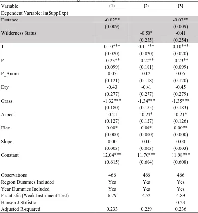
Table 1.2. The first-stage results for Model 2 including both instruments are reported in
column 3 of Table 1.3. In both models, as theory would predict, suppression expenditures are
negatively associated with a wildfire’s distance to the nearest population center in both
models. Specifically, in both models, a 10 mile increase in the distance from a fire’s point of
ignition to the nearest population center is associated with a 20 percent decrease in
suppression expenditures. A t-test indicates this relationship is statistically significant at the 5
percent significance level in both models. Similarly, I find that fires occurring in designated
wilderness areas receive less suppression expenditures than those occurring outside such
areas. Specifically, suppression expenditures are 32 percent lower for wildfires occurring in
wilderness areas.4 This result is also consistent with the theory outlined above. However, a
t-test on the individual coefficient does not show the effect as statistically significant. This is
likely due to the fact that distance and wilderness status are correlated (wilderness areas tend
to be farther away from populated areas). A joint hypothesis test using the F-statistic reveals
that one can reject the null hypothesis both coefficients are zero at the 2 percent significance
level in both models.
The second condition of a valid instrument can be tested when a model is
overidentified using the Hansen J test. The Hansen J test statistic is asymptotically distributed
as a chi-square variable with 1 degree of freedom, which implies a 10% critical value of 2.7.
The Hansen J test statistic calculated for Model 1 is 0.23 and the test statistic for Model 2 is
4 This effect was calculated, based on the reported Model 1 coefficient estimate of -0.41. Because this model
0.25. As one can see, this implies that I cannot reject the null hypothesis that the instruments
are uncorrelated with the error term at any reasonable significance level. Based on these
results, I conclude that the instruments being used meet both conditions for validity.
The strength of the instruments is tested using the procedure described in Stock and
Yogo (2005). Specifically, they show that the bias of the IV estimator relative to that of the
OLS estimator can be tested by comparing the first stage F-test statistic on the excluded
instrument to critical values that they calculated. For the purposes of this paper, I use the
Stock and Yogo method to test the null hypothesis that the maximum bias of the TSLS
estimator relative to the OLS estimator is 20%. Stock and Yogo report that the 5% critical
value for this test is 8.75 when there is a single endogenous variables and two instruments or
6.66 when there is a single endogenous variable and only one instrument. I estimate the
F-statistic on the excluded instruments for to be 4.89 for Model 1 (see table 1.2, column 3) and
4.81 for Model 2 (see table 1.3, column 3). Because neither F-statistic exceed 8.75, I cannot
reject the null hypothesis for either model. This could suggest that weak instrument problems
will be present.
One way to mitigate the bias associated with weak instruments is to use
just-identified TSLS. As Angrist and Pischke (2008) note, the just-just-identified IV estimator is
median-unbiased and unlikely to be subject to a weak-instruments critique. Therefore, in
addition to reporting overidentified TSLS estimates for Model 1 and Model 2, I will also
report TSLS estimates where only distance is used as an instrument and where only
The TSLS results for Model 1 are reported in table 1.4. As expected, I find that fires
were larger in areas that had higher temperatures in the month they ignited. Specifically, the
results for the overidentified 2SLS model indicate that a 1 degree increase in temperature is
associated with a 15 percent increase in wildfire size on average, holding everything else
constant. Results for the just-identified models are similar (see column 1 and column 2 of
table 1.4).
Also as expected, I find that fires were smaller in areas that had less precipitation in
the month the fire was ignited. Specifically, the results for the overidentified TSLS model
indicate that a 1 millimeter decrease in total precipitation during the month a fire occurs will
increase wildfire size by 32 percent on average, holding everything else constant. This result
is consistent with the notion that contemporaneous precipitation levels are most important for
fuel flammability. Again, results for the just-identified models are similar.
In addition to the contemporaneous effects of precipitation on wildfire size, we also
see that precipitation in previous periods had a significant impact on wildfire size.
Specifically, the results for the overidentified TSLS model indicate that a 1 millimeter
increase in average precipitation anomaly during the six months prior to a fire will increase
wildfire size by 58 percent on average, holding everything else constant. This result is
consistent with the notion that heavy precipitation in the months prior to a fire’s ignition can
lead to larger wildfires by creating more fine fuels. Again, results for the just-identified
The results of Model 2 are reported in table 1.5. As expected, dry ecosystems are
much more sensitive to changes in precipitation than non-dry ecosystems. One can see this
by looking at the interaction effect between precipitation anomaly and ecosystem type.
Specifically, the results for the overidentified 2SLS model indicate that a 1 millimeter
increase in the average precipitation anomaly over the 6 months prior to a fire will increase
wildfire size by 164% in dry ecosystems as opposed to only 32% in non-dry ecosystems. A
joint hypothesis test conducted using the Wald test statistic reveals that this result is
significant at the 1% significance level. Results for the just-identified models are similar.
Next I discuss the partial effect of suppression expenditures on wildfire size.The
parameter estimates discussed thus far have largely been the same regardless of whether one
considered the overidentified model or the just-identified models. This is not true when
consider the partial effect of suppression expenditures on wildfire size. Specifically,
returning to Model 1, the results for the overidentified 2SLS model indicate that a 1 percent
increase in suppression expenditures is associated with a 0.52 percent decrease in wildfire
size. By contrast, the model that only uses the wilderness status instrument indicates that a 1
percent increase in suppression expenditures is associated with a .77 percent decrease in
wildfire size. And lastly, the model that only uses the distance instrument indicates that a 1
percent increase in suppression expenditures is associated with a .38 percent decrease in
wildfire size.
Although none of these coefficient estimates are statistically significant, the estimate
case for two reasons. First, it is the result of a just-identified model and therefore
median-unbiased. Second, the F-statistic from the first-stage results of this model is significantly
higher than the F-statistic from the first-stage results of the model only using the wilderness
status instrument (see column 1 of table 1.2). In fact, the F-statistic for this model, 6.79,
exceeds the previously mentioned Stock and Yogo critical value. Both of these facts suggest
that bias associated with weak instruments is less of a problem with this model than any of
the others.
In addition to the TSLS estimates of Models 1 and 2, I also provide OLS estimates of
each model in table 1.3 in column 2 and 3 respectively. As one can see, the OLS estimates
are markedly different from the estimates obtained by TSLS. Specifically, the sign on the
coefficient for suppression effort is also positive and strongly significant, which is the
opposite of how we would expect suppression to influence wildfire size. Similarly, the
wildfire size seems less sensitive to changes in temperature and wildfire size when looking at
the OLS estimates than the TSLS estimates. This is not what we would expect from two
consistent estimators. A Wu-Hausman test formally confirms that we reject the null
hypothesis that the OLS estimates are consistent at the 5% level. This result conforms with
the expectation that wildfire size and suppression effort are jointly determined.
The results presented in this paper can be of great use to USFS policy makers that
want to anticipated how higher temperatures from Climate Change will influence wildfire
size. For example, according to the PCM-B2 and HadCM3 climate models, temperatures in
the western United States are expected to increase between 1.6 C and 6.3 C in the period
2070 to 2100 relative to temperatures in the 1970-2000 period (McKenzie, 2004). Across
several different model specification, the results presented in this paper predict that a 1 C
increase in temperature will increase mean wildfire size by 13%. Therefore, increase in
temperature between 1.6 C and 6.3 C would imply mean wildfire size will increase by 20%
to 80%.
To put this into perspective, we can calculate a lower-bound for how much
suppression expenditures would have to increase to offset this increase in wildfire size.
Specifically, using the preferred model where only the distance instrument is used, we can
construct a 95% confidence interval for the population parameter for the coefficient
ln(SuppExp) that ranges from -1.24 to 0.47. Using the lower bound of this interval suggests
that if the USFS wanted to increase suppression efforts to completely offset an increase in
wildfire size of 20-79% they would need to increase suppression expenditures by at least
16-63%. In my dataset, mean suppression expenditures was estimated to be $3.3 million. This
means suppression costs on the average wildfire could increase $0.5-$2 million.
It is important to understand the limitations of these results. Specifically,
these results hold fuel and ecosystem characteristics constant, when in fact these might
being removed from national forests over the long run, which could mitigate the effects of
higher temperatures on wildfire size. Measuring the importance of such changes is beyond
the scope of this study, but they do suggest that caution should be taken when using these
results to extrapolate impacts of climate changes in the distant future.
1.8. Figures and Tables
Data Source: Headwater Economics, 2015
Figure 1.2. Total Timber Cut on USFS land by Region 1980-2013
0 2 0 0 0 4 0 0 0 6 0 0 0 Bi lli o n s o f Bo a rd F e e t
1980 1985 1990 1995 2000 2005 2010 2015
Year
Region 1 Region 3
Region 4 Region 5
Table 1.1. Descriptive Statistics Variable
N Mean Standard
Deviation Minimum Maximum
Size (Hectares) 466 4,082.67 11,183.57 40.46 113,333.70
T 466 19.36 4.49 1.91 29.42
P 466 1.57 0.87 0.02 5.19
P_Anom 466 0.22 0.81 -3.26 3.59
SuppExp 466 3,366,152.00 7,129,091.00 1,305.31 98,700,000.00
Dry 466 0.21 0.41 0.00 1.00
Grass 466 0.36 0.48 0.00 1.00
Aspect 466 -0.13 0.72 -1.00 1.00
Elevation 466 5,284.74 1,971.12 43.00 10,000.00
Slope 466 38.95 23.93 0.00 150.00
USFS Region 3 466 0.20 0.40 0.00 1.00
USFS Region 4 466 0.25 0.43 0.00 1.00
USFS Region 5 466 0.20 0.40 0.00 1.00
USFS Region 6 466 0.17 0.37 0.00 1.00
2003 466 0.02 0.15 0.00 1.00
2004 466 0.15 0.35 0.00 1.00
2005 466 0.18 0.39 0.00 1.00
2006 466 0.34 0.47 0.00 1.00
Table 1.2. Results from First-Stage of TSLS Regression for Model 1
Variable (1) (2) (3)
Dependent Variable: ln(SuppExp)
Distance -0.02** -0.02**
(0.009) (0.009)
Wilderness Status -0.50* -0.41
(0.255) (0.254)
T 0.10*** 0.11*** 0.10***
(0.020) (0.020) (0.020)
P -0.23** -0.22** -0.23**
(0.099) (0.101) (0.099)
P_Anom 0.05 0.02 0.05
(0.121) (0.118) (0.120)
Dry -0.43 -0.41 -0.45
(0.277) (0.277) (0.279)
Grass -1.32*** -1.34*** -1.35***
(0.180) (0.185) (0.183)
Aspect -0.21 -0.24* -0.21*
(0.127) (0.127) (0.126)
Elev 0.00* 0.00* 0.00**
(0.000) (0.000) (0.000)
Slope 0.00 0.00 0.00
(0.003) (0.003) (0.003)
Constant 12.04*** 11.70*** 11.98***
(0.615) (0.604) (0.608)
Observations 466 466 466
Region Dummies Included Yes Yes Yes
Year Dummies Included Yes Yes Yes
F-statistic (Weak Instrument Test) 6.79 4.52 4.89
Hansen J Statistic 0.23
Adjusted R-squared 0.233 0.229 0.236
Table 1.3. Results from First-Stage of TSLS Regression for Model 2
Variable (1) (2) (3)
Dependent Variable: ln(SuppExp)
Distance -0.02** -0.02**
(0.009) (0.009)
Wilderness Status -0.49* -0.40
(0.256) (0.255)
T 0.10*** 0.10*** 0.10***
(0.020) (0.021) (0.020)
P -0.24** -0.24** -0.24**
(0.100) (0.102) (0.100)
P_Anom -0.03 -0.06 -0.03
(0.129) (0.127) (0.128)
P_Anom x Dry 0.32 0.32 0.31
(0.205) (0.207) (0.208)
Dry -0.44 -0.42 -0.46*
(0.276) (0.277) (0.279)
Grass -1.35*** -1.36*** -1.37***
(0.179) (0.183) (0.181)
Aspect -0.20 -0.23* -0.21
(0.127) (0.127) (0.126)
Elev 0.00* 0.00* 0.00**
(0.000) (0.000) (0.000)
Slope 0.00 0.00 0.00
(0.003) (0.003) (0.003)
Constant 12.10*** 11.76*** 12.03***
(0.615) (0.605) (0.608)
Observations 466 466 466
Region Dummies Included Yes Yes Yes
Year Dummies Included Yes Yes Yes
F-statistic (Weak Instrument Test) 6.73 4.39 4.81
Hansen J Statistic 0.25
Adjusted R-squared 0.234 0.230 0.237
Table 1.4. TSLS Estimation Results for Wildfire Size Model 1
Variable (1) (2) (3)
Dependent Variable: ln(Size)
Instrumental Variable: Distance Only
Wilderness Status Only
Distance & Wilderness Status
ln(SuppExp) -0.38 -0.73 -0.52
(0.457) (0.774) (0.455)
T 0.12** 0.16* 0.14**
(0.054) (0.085) (0.054)
P -0.37** -0.45* -0.40**
(0.164) (0.241) (0.175)
P_Anom 0.46*** 0.47** 0.46***
(0.163) (0.198) (0.175)
Dry -0.28 -0.41 -0.33
(0.413) (0.542) (0.439)
Grass -1.26* -1.72* -1.43**
(0.644) (1.026) (0.637)
Aspect 0.06 -0.02 0.03
(0.180) (0.251) (0.189)
Elev 0.00 0.00 0.00
(0.000) (0.000) (0.000)
Slope 0.01 0.01 0.01
(0.005) (0.006) (0.005)
Constant 10.92** 15.05 12.49**
(5.425) (9.189) (5.436)
Observations 466 466 466
Region Dummies Included Yes Yes Yes
Year Dummies Included Yes Yes Yes
Table 1.5. TSLS Estimation Results for Wildfire Size Model 1
Variable (1) (2) (3)
Dependent Variable: ln(Size)
Instrumental Variable: Distance Only
Wilderness Status Only
Distance & Wilderness
Status
ln(SuppExp) -0.39 -0.77 -0.50
(0.461) (0.807) (0.461)
T 0.12** 0.16* 0.13**
(0.053) (0.087) (0.054)
P -0.40** -0.49* -0.42**
(0.171) (0.258) (0.182)
P_Anom 0.30* 0.27 0.28
(0.177) (0.216) (0.190)
P_Anom x Dry 0.66** 0.78* 0.69**
(0.331) (0.437) (0.349)
Dry -0.31 -0.46 -0.35
(0.417) (0.562) (0.445)
Grass -1.32** -1.81* -1.47**
(0.655) (1.084) (0.654)
Aspect 0.07 -0.02 0.04
(0.180) (0.254) (0.190)
Elev 0.00 0.00 0.00
(0.000) (0.000) (0.000)
Slope 0.01 0.01 0.01
(0.005) (0.006) (0.005)
Constant 10.24* 14.68 11.51**
(5.510) (9.621) (5.539)
Observations 466 466 466
Region Dummies Included Yes Yes Yes
Year Dummies Included Yes Yes Yes
Wald Statistic (Joint Hypothesis Test) 11.30*** 7.87*** 10.16***
Table 1.6. OLS Estimation Results for Wildfire Size Models 1 and 2
Variable (1) (2)
Model 1 Model 2
Dependent Variable: ln(Size)
ln(SuppExp) 0.65*** 0.64***
(0.043) (0.043)
T 0.02 0.02
(0.016) (0.016)
P -0.14* -0.15**
(0.075) (0.077)
P_Anom 0.44*** 0.36***
(0.106) (0.110)
P_Anom x Dry 0.31
(0.203)
Dry 0.12 0.10
(0.235) (0.235)
Grass 0.08 0.06
(0.164) (0.165)
Aspect 0.30*** 0.30***
(0.095) (0.095)
Elev -0.00 -0.00
(0.000) (0.000)
Slope 0.00 0.00
(0.003) (0.003)
Constant -2.06*** -1.96***
(0.710) (0.712)
Observations 466 466
Region Dummies Included Yes Yes
Year Dummies Included Yes Yes
Wald Statistic (Joint Hypothesis Test) 9.42***
1.9 References
Angrist, Joshua D., and Jörn-Steffen Pischke. Mostly harmless econometrics: An empiricist's companion. Princeton university press, 2008.
Bracmort, Kelsi. “Wildfire Fuels and Fuel Reduction”. Congressional Research Service. Available at http://nationalaglawcenter.org/wp-content/uploads/assets/crs/R40811.pdf
Calef, M. P., A. D. McGuire, and F. S. Chapin III. "Human influences on wildfire in Alaska from 1988 through 2005: an analysis of the spatial patterns of human impacts." Earth Interactions 12, no. 1 (2008): 1-17.
Donovan, Geoffrey H., and Douglas B. Rideout. "A reformulation of the cost plus net value change (C+ NVC) model of wildfire economics." Forest Science 49, no. 2 (2003): 318-323.
Farnham, Timothy J., and Paul Mohai. "National Forest timber management over the past decade." Policy Studies Journal 23, no. 2 (1995): 268-280.
Flannigan, M., Krawchuck, M., de Groot, W., Wotton, B. & Gowman, L. “Implications of changing climate for global wildland fire.” International Journal of Wildland Fire. vol. 18 (2009): 483-507.
Headwater Economics. “National Forest Timber Sales and Timber Cuts, FY 1980-2013.” Accessed April 15, 2015. Available at <http://headwaterseconomics.org/interactive/national-forests-timber-cut-sold.
Husari, Susan J., and Kevin S. McKelvey. "Fire management policies and programs." In
Sierra Nevada ecosystem project: final report to Congress, vol. 2, pp. 1101-1118. (1997). Accessed April 15, 2015. Available at
<http://pubs.usgs.gov/dds/dds-43/VOL_II/VII_C40.PDF>
Johnston, J. and Klick, J. “The Political Economy of Wildfire Management: Saving Forests, Saving Houses, or Burning Money” In Wildfire Policy: Law and Economics Perspectives. Edited by Karen M. Bradshaw and Dean Lueck. RFF Press. (2011)
J. H. Lawrimore, M. J. Menne, B. E. Gleason, C. N. Williams, D. B. Wuertz, R. S. Vose, and J. Rennie (2011), An overview of the Global Historical Climatology Network monthly mean temperature data set, version 3, J. Geophys. Res., 116, D19121,
Littell, J., McKenzie, D., Peterson, D. & Westerling, A. “Climate and wildfire area burned in western U.S. ecoprovinces, 1916-2003.” Ecological Applications. vol. 19 (2009): 1003-21.
McKenzie D, Gedalof Z, Peterson D, and Mote P. “Climate Change Wildfire, and Conservation.” Conservation Biology. vol. 18 no. 4 (2004): 890-902
National Interagency Fire Center (NIFC). “Total Wildland Fires and Acres (1960-2009)”. (2014) Accessed January 16, 2015. Available at
<http://www.nifc.gov/fireInfo/fireInfo_stats_totalFires.html.>
Natural Resources Law Center. “Special Use Provisions in Wilderness Legislation.” Accessed April 15, 2015. Available at
<http://www.wilderness.net/toolboxes/documents/MSP/Spec.%20Use%20Provisions%20in %20Legislation.pdf.>
Prestemon, J. P., Hawbaker, T. J., Bowden, M., Carpenter, J., Scranton, S., Brooks, M. T., et al. “Wildfire ignitions: A review of the science and recommendations for empirical modeling. USDA Forest Service General Technical Report SRS-171”. (2013). Available at < http://www.srs.fs.usda.gov/pubs/42766 >
Stock, James H., and Motohiro Yogo. "Testing for weak instruments in linear IV
regression." Identification and inference for econometric models: Essays in honor of Thomas Rothenberg 1 (2005).
Routlet N, Moore T, Bubier J, and Laufluer P. “Northern fens - methane flux and climate change.” Tellus B vol.44 (1992): 100-105.
United States Forest Service (USFS). "Wildfire, Wildlands, and People: Understanding and Preparing for Wildfire in the Wildland-Urban Interface." (2013). Accessed January 16, 2015. http://www.fs.fed.us/openspace/fote/reports/GTR-299.pdf
Westerling, A. L., and B. P. Bryant. "Climate change and wildfire in California." Climatic Change 87, no. 1 (2008): 231-249.