The Use of Extrapolation in
Computing Color Look-Up
Tables
S. A. Rajala
A. P. Kakodkar
<Center for Communications
and
Signal Processing
Department of Electrical
and
Computer Engineering
North Carolina State University
The use of extrapolation in computing color look-up
tables
Sarah A. Rajala, H. Joel Trussell, Atish P. Kakodkar
Dept. of Electrical and Computer Engineering
North Carolina State University
Raleigh, NC 27695-7911
ABSTRACT
Colorimetric reproduction requires calibrated color output devices. One way to characterize a color output device is with a three-dimensional look-up table which maps the tristimulus values, t, to the control values, c of the output device. The functional form of the output device can be written in vector notation as t
=
F(
c). The purpose of calibration is to define an inverse mapping from tristimulus values to control values. Since the functionF(.)
has no closed form, it is defined by interpolation from a table of values.Given a set of control values
{Ci}
on a regular grid and the corresponding set of tristimulus values{t,}
obtained from data collection, we wish to find the{c
g } for different {tg } on a grid in the tristimulus space.The gridis obtained from a relatively sparse data set with an appropriately defined interpolation scheme. This interpolation scheme can be complex since it is used only once to compute the grid. The regular finer grid can be used in real-time with simple interpolation.
While the functions which represent the device are usually well behaved and smoothly varying, the trun-cation of the data can cause a problem with interpolations near the edge of the gamut. An approach to solving this problem is to extrapolate the data outside the gamut using bandlimited or linear extrapolation methods. The extrapolated points along with the measured data are used in a single interpolation algorithm over the entire gamut of the device. The results of this method are comparable to other interpolation methods but it is simpler to implement. It has the additional advantage of allowing physical constraints, such as bandlimits, to be easily imposed.
1
INTRODUCTION
One of the applications of this work is the calibration of nonlinear printing devices. For this research, we use the proposed color data interpolation scheme to calibrate a Kodak XL7700 thermal dye transfer printer. To determine the appropriate color interpolation scheme, a forward model for the printerisdefined and interpolation schemes are evaluated using simulated data. In particular, we realize that while the functions which represent the device are well behaved and smoothly varying, the truncation of the data can cause a problem with interpolations near the edge of the gamut. An approach to solving this problem is to extrapolate the data outside the gamut and use these points in a single interpolation algorithm over the entire gamut of the device. The results using these extrapolated points are discussed in this paper.
2
THE FORWARD MODEL
A printing process is subtractive in nature. Each of the cyan, magenta and yellow dyes removes an amount of its complimentary color, red, green and blue, respectively. The amount of a particular color removed is related to the concentration of the dye. Each dye is characterized by its density D(,\) at any wavelength '\. The density is proportional to the concentration c of the dye. Therefore",
i
=
1,2,3(1)
where Di,Tnaz isthe density at unit concentration for dye iand c; is the concentration of dye i. Transmission of a particular dye is related logarithmically to its density as
i=1,2,3
(2)
The observed spectrum at a particular wavelength ,\is given as2
(3)
where 11('\) is the transmission of the it h dye at wavelength ,\ and 1(,\) is the intensity of the illuminant at wavelength '\. The effect of paper or the transparency has been neglected by assuming it to be uniform. Using equation
(2),
equation (3) may be rewritten as:(4)
Thus the forward model can be written mathematically as
,
2(5)
where L is a NzN diagonal matrix representing the illuminant spectrum, c is the 3-vector representing the concentration of the dyes and g is the N-vector representing the radiant spectrum. The concentration values must be between zero and unity and the Nz3 matrix of density spectra Dm a 22 represents the densities at the
maximum concentration. This model ignores any nonlinear interactions between the colorant layers. The tristimulus values zyz are obtained by the equation
(6)
where A is a Nz3 matrix of the CIE color matching functions. The (x,y,z) value~ are th:n converted to the
t=F(c)
Control Values Color Space
Figure 1: The Forward Model
3
DEVELOPING THE LOOK-UP TABLE
Using the mathematical model, a coarse 8x8x8 look-up table mapping the control values to the output CIE
L·a·b· values is generated with the forward model of equation
(5).
This forward model is used for testing only and to help us predict how well each of the interpolation functions willperform for the ideal model. We havet
=
F(c)
(7)
where t is a 3-vector of the CIE L·a·b· values and c is a 3-vector of the control values. The forward modelis
shown in Figure 1.
(9)
-3< z <
.=.!2 - - 2
.=.!.<z<!
2 - - 2.J.<z<~2 - - 2
A finer regular grid isconstructedinthe CIE L·a·bt
space. For a certain CIEL·a·b· vector tgon this finer regular grid the corresponding control vector cg isobtained. Iterative techniques with interpolation are used to estimate the control vector corresponding to every vector tg on the finer grid. For a given CIE L·a·b· vector
tg, an initial estimate Co of the control vector is made and the corresponding CIE L·atbt vector is obtained by interpolating over the three dimensional regular grid of control values. Newton's method'[ in three dimensions is used to obtain a new estimate of the control value. This procedure is equivalent to finding a root of the equation
f(c)
=
t
g 01'f(c) -
tg
=
0
(8)
where the functionf refers to the interpolating function that is used. This iteration is carried out until equation (8) is solved to the selected degree of accuracy.
Two kinds of interpolating functions were used, the bell function and the cubic B-spline function. A bell interpolating function is obtained by the convolution of a triangle function with a square function and is defined ass:
A cubic B-splineis defined as5:
{
1
+
!lzl2- z3 0~
Izi
~ 1S,,(z) =
3
~(22
_Iz13)
1
~
Izi
~
2(10)
Three-dimensional separable interpolation is used to interpolate for the CIE L·a·b· values t,
=
(t,.ll t,.21
t,.3)
on the finer gridt
g ., (Cl,C2, C3)=
I:I:I:
w,(i,i, k)S(Cl - i)S(C2 - i)S(C3 - k)
Ie j
. . . .
.
.
. . . .
.
.
.
.
....
~
-t , ,
~
..,...•....
....
~..
: : :
:
: : : :...
~.
....t-..
...t- .
...
..
.
...
..
...
·..·t..
. .
....+-..
.
,
...
.
..
~
.
....
~..
...~
.
....•..
~
..•..•..
~ ~
..•...
~
..
~
.
~
; ; ; ;
~ ~ ~ ~ ~Control value space
• Points to be Extrapolated
Figure 2: Extrapolation in the Control Value Space
where wl(i,
i,
k) are the weights used to interpolate, Sdenotes the interpolation function used and (el' C2, C3)denotes the control vector. In order to determine the weights, the interpolated values are set to the measured values on the coarse grid.
These interpolation schemes assume the presence of a sufficient number of data points close to the inter-polated point. However, the truncation of the data can cause a problem with interpolations near the boundary of the printer gamut. In order to solve this problem, we extrapolate the data set for points outside the gamut (Figure 2). These extrapolated points are then used in an interpolation algorithm which does not require treating the boundary as a special case. Two types of extrapolation schemes were proposed (i) simple linear extrapolation and
(ii)
band-limited extrapolation. The latter scheme was proposed since the mapping from the CMY colorants to the CIE L*a·b"space is usually well-behaved and smoothly varying.Both the extrapolation schemes were implemented in a one-dimension problem to compare the relative errors that occurin the interpolation of points close to the boundary. A series of lines were created by keeping two colorants constant and varying the third. The true L· values corresponding to these control values are compared with the original
L·
values to calculate the error. Figure 3compares typical errors due to both the schemes. It is observed that the linear extrapolation gives better results for all simulations.Linear extrapolation is more attractive than the band-limited extrapolation scheme since it is much easier to implement and takes less time. Band-limited extrapolation has the advantage of allowing physical constraints to be imposed. However, since an iterative algorithrn'' is used, it has the disadvantage of taking a long time and not giving significantly different results obtained by linear extrapolation.
The points obtained by linear extrapolation are then used in the mathematical model to create a finer, regular LUTin the CIE
L·
a·b·
space. The bell and the spline interpolation functions perform almost identically. As a result, the bell function, which showed a smaller average LlE error, was used in the actual printer calibrationError for L Curve
0.3 ...
--.--r----,---r----,----r---,..--....---Cone of yellow. 0.5714 Cone of magenta. 0 5714
09
08 _ _ using band-limited extrapolation --- using linear extrapolation
0.3 0.4 0.5 0.6 07
Concentration
0'
Cyan02 0.1
0.05
0.1
g
0.15w
Figure 3: Errors due to Extrapolation
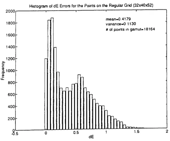
Histogram of dE Errors for the Points onthe Regular Grid (32x40x52)
2
1.5 dE
0.5 o
mean-0.4179
vananca-O1130
#of pomtsIngamut.18164
I
~
-8.5
400200 800
600 laoo
1400 1600 2000
1200
~
c
~1000
Q)
u:
2 15
dE
05
o
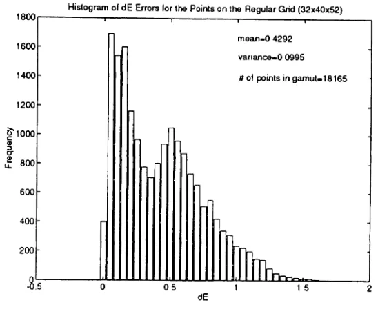
Histogram of dE Errors for the Points ontheRegular Grid (32x40x52) mean-Q 4292
varlance-O 0995
#of points in gamut.18165
~
200
400
600
-8.5
1400 1600 18001200 g1000
Q) ::J
0-tt
800Figure 5: ~E Errors Using Spline Interpolation
4
THE PRINTER CALIBRATION
A calibration chart was generated from the KODAK XL7700 by dividing the control value space into eight equi-spaced samples in each dimension to generate 512 color patches. A GRETAG SPM-50 spectrophotometer was used to measure the elE L·a·b· values of these color patches. This set of CIE L·a·b· values forms the known coarse data set.
It was noticed that the ~E errors between two color patches corresponding to identical control values was significant when they were printed in different regions of the printer paper. This indicated that the printer needed to be calibrated for each of its heads. Another observation was that there was a significant difference between the ~E errors between two color patches corresponding to identical control values when they were printed on different sheets. This meant that the coarse LUT had to be created out of an average over several printouts. The standard deviation over different sheets ranged from 1.06LlEto 1.93LlE. This provides a lower bound on the accuracy of the calibration.
Making use of the above observations, the printer was calibrated for only one of its heads. The 8x8x8 LUT was measured and averaged over several printouts. As mentioned earlier, extrapolation of points at the boundary of the printer gamut was used in the interpolation routine to create the finer, regular LUT in the CIE
L·
a·b·
space.Using the bell interpolation function, a finer regular grid was created in the CIE
L·
a·b"
space. Trilinear interpolation isused to find control values not on the finer grid. To measure the average interpolation error that was obtained, a test pattern of 343 points (corresponding to all combinations of the three dyes by varying their concentrations from 0.2 to 0.8 in steps on 0.1) were used. The testing procedure is described schematically inFigure 6. The test pattern whose control values are known is printed and its CIE Lt a tb· values are measured
by the spectrophotometer. These CIE
L·
a tb"
values are then used in the interpolation routine to obtain theGretag SPM-50
CIE L*a*b* vaJuas
Interpolation Process
Test
Chart CIE L*a*b*
vaJues
CaJculate L*a*b* error
I
CIE L*a*b-values,....,.-r-r-"lr-T""'T"""'I"'...
Gratag SPM-50
Calibrated
Chart
Figure 6: Testing the Interpolation Scheme
obtained by the calibrated printer.
A simple algorithm was used to divide the CIE L·a·b· space into an equi-spaced grid. A minimum grid size of 32 was used in each direction. The spacing in the grid was calculated in the following manner:
1. divide the range in each of the L·, a· and b· directions (obtained from the 8x8x8 LUT) by the minimum grid size i.e. form the spacings
(L:naz - L:nin)/31, (a:naz - a:nin)/31
and(b:naz - b:nin)/31.
2. choose the minimum of the spacings formed above as the spacing between two points on the finer grid in
the CIE L·a·b· space.
Once this LUT (mapping points on a finerJ regular grid in the CIE L·a·b"space to the control value space)
is created, we can use it with simple trilinear interpolation to estimate the control values for any CIE L·a·b"
point in the printer gamut. If the mapping from the control value space to the CIE L·atbt space isassumed to be smoothly varying, and if the size of the uniform grid in CIE L·atb· is sufficiently fine then we can assume that the contribution to the error due to the trilinear interpolation will not be large. Since both these conditions are satisfied in our case, we hope to observe that trilinear interpolation does not increase the dE errors by a large factor.
To test out our hypothesis, we use the same test print consisting of 343 equi-spaced samples and measure their CIE
L·a·b·
values. Using trilinear interpolation over the fine, regular grid that we have created we estimate the control values for each of the test points. These control values are then used to print a new chart whose CIEL·a·b·
values are measured again. The CIE L·atbt values of the color patches on this sheet are compared with the CIEL·
a·b·
values of the color patches of the test sheet and the dE errors are calculated. These results are discussed in the next section. The procedure is described in Figure 6. The interpolation procedure now, refers to trilinear interpolation.~
Gamut Surface Control vaJue for b is to be obtained by extrapolation• Grid Points
~:: Test Point
Figure 7: Extrapolation to Cover Entire Gamut
not be interpolated with the grid that we have (Figure 7). However, this is a serious problem since we would like to make sure that we can print all points lying in the printer gamut. To overcome this problem, points on such cubes which are outside the printer gamut should be assigned control values (outside the printer range, obviously) by extrapolation. This problem will be looked atin the near future and will be an additional source of error for points close to the boundary of the printer gamut.
5
EXPERIMENTAL RESULTS
The D.E errors due to the interpolation rou tine used to create the fine, regular grid in the CIE L·a·b·
space are calculated and the relevant statistics are tabulated in Table 1. Figure 8 shows a histogram of these
dE errors.
Table 1: ~E Errors Due to Interpolation Statistics BellFunction
Max 6.E 5.5391
Average LlE 2.0452 Variance dE 0.5776
Using
the
same test pattern as the one used to measure the error in creating the grid, we measure the average... _ ... An.a. 4-_ ...~l;Tuu'llP ;"+~pnnJtllt.lnn Wp ("~n nTp.rli~t that the error that is added bv the trilinear internolation
5
EXPERIMENTAL RESULTS
The D.E errors due to the interpolation rou tine used to create the fine, regular grid in the CIE L·a·b·
space are calculated and the relevant statistics are tabulated in Table 1. Figure 8 shows a histogram of these
dE errors.
Table 1: ~E Errors Due to Interpolation
~
StatisticsI
Bell Function~
Histogram of dE Errors
2 5 1 - - - . - - - r - - - . - - - -...
---r---~---mean -2.0452
vanance - o.sns
20
15
~
c
a>
:)
xr
Q)
tt 10
5
2
~rrJhn
nn
3 4 dE
s
m
s 7Figure 8: dE Errors Due to Interpolation
7
6
5
4 dE
3
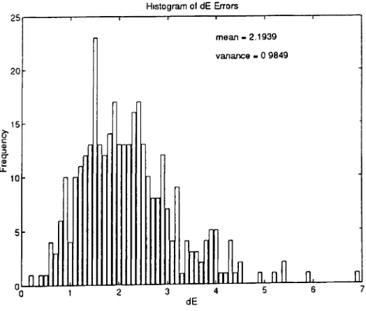
Histogram of dE Errors
2
5
mean - 2.1939 vanance • 0 9849
I
r
I
I
nm
I
~ rn~
n
n~
n
n
520 2
15
~
c Q) :)
sr
Q)
u:
10
Table 2: aE Errors Due to Trilinear Interpolation Statistics Bell Function
Max aE 6.9392
Average dE 2.1939 Variance dE 0.9849
the dE errors increased almost two-fold. The histogram of the LlE errors is plotted in Figure 9. The standard deviation of the printer over different sheets was about l.64LlE which is of the same order as the average dE of 2.1939 that was obtained after trilinear interpolation.
6
CONCLUSION
The printer was calibrated for a single print head. The extrapolated points were used along with the measured values to reduce the interpolation errors for points close to the boundary of the printer gamut. The look-up table method with trilinear interpolation worked well and showed that little could be gained by using more precise interpolation methods for all points. The average LlE errors due to the interpolation methods are of the same order as the variability of the printer. Therefore, no significant improvement in the average dE errors may be expected by changing the interpolation scheme. The interpolation functions that were used seem to be good choices for the calibration of the KODAK XL7700 thermal dye transfer printer.
References
[1] Hunt, R. W. G., The Reproduction of Colour in Photography, Printing &Television, Fountain Press, Eng-land, 1987.
[2] Trussell, H. J., and Sullivan, J. R., A Vector Space Approach to Color Imaging System" Proceedings, SPIE Conference on Image Processing Algorithms and Techniques, Santa Clara, CA, 12-14Feb. 1990.
[3] Wyszecki, G. and Stiles, W. S., Color Science: Concepts and Methods, Quantitative Data and Formulae, John Wiley and Sons, 1982.
[4] Dennis, J.E. and Schnabel, R.B., Numerical Methods for Unconstrained Optimisation and Non-Linear Equations, Englewood Cliffs, N.J., Prentice Hall, 1983.
[5] Pratt, W. K., Digital Image Processing, John Wiley and Sons, 1991.