On compressible pairings and their computation
Michael Naehrig1⋆, Paulo S. L. M. Barreto2⋆⋆, and Peter Schwabe1 1
Department of Mathematics and Computer Science
Technische Universiteit Eindhoven, P.O. Box 513, 5600 MB Eindhoven, Netherlands
{michael,peter}@cryptojedi.org 2
Escola Polit´ecnica, Universidade de S˜ao Paulo. Av. Prof. Luciano Gualberto, tr. 3, n. 158.
BR 05508-900, S˜ao Paulo(SP), Brazil.
Abstract. In this paper we provide explicit formulæ to compute bilin-ear pairings in compressed form. We indicate families of curves where the proposed compressed computation method can be applied and where par-ticularly generalized versions of the Eta and Ate pairings due to Zhaoet al.are especially efficient. Our approach introduces more flexibility when trading off computation speed and memory requirement. Furthermore, compressed computation of reduced pairings can be done without any fi-nite field inversions. We also give a performance evaluation and compare the new method with conventional pairing algorithms.
Keywords:pairing-based cryptography, compressible pairings, algebraic tori, Tate pairing, Eta pairing, Ate pairing, twists.
1
Introduction
Cryptographically relevant bilinear maps like the Tate and Weil pairing usually take values over an extension field Fpk of the base fieldFp. Pairing inputs are
typically points on an elliptic curve defined over Fp. It has been known for a
while (see the work of Scott and Barreto [13] and Granger, Page and Stam [7]) that pairing values can be efficiently represented in compressed form by using either traces over subfields or algebraic tori. The former approach leads to a small loss of functionality: the trace of an exponential, Tr(gx), can be computed from the trace Tr(g) and the exponent x alone, but the trace of a product Tr(gh) cannot be easily computed from Tr(g) and Tr(h). The latter approach does not suffer from this drawback, since torus elements can implicitly be multiplied in the compressed representation. With either approach, pairing values can be
⋆
Most of the work presented in this paper was done, while the first author was visiting the Escola Polit´ecnica, Universidade de S˜ao Paulo, Brazil. The visit was supported by the German Research Foundation (DFG).
⋆⋆ Supported by the Brazilian National Council for Scientific and Technological
efficiently compressed to one half or one third of the original length, depending on the precise setting of the underlying fields and curves.
Our contribution in this paper is to provide explicit formulæ to compute pairings directly in compressed form. Although we do not claim any perfor-mance improvement over existing methods, we show that full implementation of arithmetic overFpk can be avoided altogether; only operations for manipulating pairing arguments and (compressed) pairing values are needed.
From an implementor’s or hardware designer’s perspective the contribution of this paper consists of mainly two aspects. Firstly, the explicit formulæ for multiplication and squaring of torus elements give more flexibility in trading off computation speed with memory requirement. The second aspect concerns field inversions during pairing computation. Using projective representation for curve points, inversions can be avoided in the Miller loop. However, a very efficient way to then compute the final exponentiation is to decompose the exponent into three factors and use the Frobenius automorphism to compute powers for two of these factors. This involves an inversion in Fpk, which can be avoided using the compressed representation of pairing values. Hence, we can entirely avoid field inversion during pairing computation and still use fast Frobenius actions in the final exponentiation. From a more theoretical perspective this approach can be seen as a first step to further enhancement of the resulting algorithms, and parallels the case of hyperelliptic curve arithmetic where the introduction of explicit formulæ paved the way to more efficient arithmetic.
We provide timing results for implementations of different pairing algorithms, comparing the newly proposed pairings in compressed form with their conven-tional counterparts. Addiconven-tionally, we give examples of curve families amenable to pairing compression where generalized versions of the Eta and Ate pairings due to Zhaoet al.are more efficient than the non-generalized versions. We pro-vide examples for the three AES security levels 128, 192 and 256 bits. In this paper we use the notion Eta pairing instead of twisted Ate pairing, because it has originally been used in the non-supersingular case as well.
This paper is organized as follows. In Sections 2 and 3 we review mathe-matical concepts related to pairings and algebraic tori. In Section 4 we discuss torus-based pairing compression and provide explicit formulæ for pairing com-putation in compressed form. We describe how to avoid inversions in Section 5. In Section 6 implementation costs are given and we conclude in Section 7.
2
Preliminaries on pairings
LetEbe an elliptic curve defined over a finite fieldFpof characteristicp≥5. Let
rbe a prime divisor of the group ordern= #E(Fp) and letkbe the embedding
degree ofE with respect tor, i.e. kis the smallest integer such thatr|pk−1.
We assume thatk >1.
LetFq be an extension ofFp. An elliptic curveE′ over Fq is called a twist
curves regarding their existence and the possible group orders of E′(F
q) given
by Hess, Smart and Vercauteren in [8].
We consider an r-torsion pointP ∈E(Fp)[r] and an independent r-torsion
pointQ∈E(Fpk)[r]. We fixG1=hPi ⊆E(Fp)[r] andG2=hQi ⊆E(Fpk)[r]. If the curve has a twist of orderdwe may choose the pointQarising asQ=ψd(Q′),
where Q′ is an F
pk/d-rational point of order r on the twist E′, see again [8]. Taking this into account we can represent points inhQiby the points in hQ′i ⊆
E′(F
pk/d)[r]. Lett be the trace of Frobenius onE/Fpandλ= (t−1)k/dmodr. Notice that λis a primitive d-th root of unity modulor.
Thei-th Miller function fi,P forP is a function with divisor (fi,P) =i(P)−
([i]P)−(i−1)(O). We use Miller functions to compute pairings. Let the function esbe defined by
es:G1×G2→µr, (P, Q)7→fs,P(Q)(p
k−1)/r .
For certain choices of s this function is a non-degenerate bilinear pairing. For s = r we obtain the reduced Tate pairing τ, s = λ yields the reduced Eta pairingηands=T =t−1 leads to the reduced Ate pairingαby switching the arguments. Altogether we have
– Tate pairing:τ(P, Q) =fr,P(Q)(p
k−1)/r , – Eta pairing:η(P, Q) =fλ,P(Q)(p
k
−1)/r,
– Ate pairing:α(P, Q) =fT,Q(P)(p
k−1)/r .
To obtain unique values, all pairings are reduced via the final exponentiation by (pk−1)/r. The Eta pairing was introduced in the supersingular context by
Bar-reto, Galbraith, ´O’ h´Eigeartaigh and Scott in [1]. The Ate pairing was introduced by Hess, Smart and Vercauteren [8]. Actually the concept of the Eta pairing can be transferred to ordinary curves as well. Hess, Smart and Vercauteren [8] call it the twisted Ate pairing.
Recently much progress has been made in improving the performance of pairing computation. Main achievements have been made by suggesting variants of the above pairings which shorten the loop length in Miller’s algorithm, for example so called generalized pairings [15], optimized pairings [11], the R-Ate pairing [10] as well as optimal pairings [14].
As an example we consider the generalized versions of the Eta and Ate pair-ings by Zhao, Zhang and Huang [15]:
– generalized Eta pairing:ηc(P, Q) =fλcmodr,P(Q)(p k−1)/r
, 0< c < k, – generalized Ate pairing:αc(P, Q) =fTcmodr,Q(P)(p
k−1)/r
, 0< c < k.
For a certain choice of c the loop length of the generalized pairings may turn out shorter than the loop length of the original pairing. Notice that if Tc≡ −1
(mod r) orλc ≡ −1 (modr) the loop length isr−1 which is the same as for
the Tate pairing and does not give any advantage.
of the loop length. The examples all have embedding degree divisible by 6 and a twist of degree 6 such that the compressed pairing computations of Sections 4 and 5 can be applied. We stress that for all example families the generalized Eta pairing is more efficient than the Tate pairing. We emphasize the Eta pairing since this goes along with our compression method, but we note that there are versions of the Ate pairing which have a much shorter loop length than the pairings suggested here. For example the curves in Example 1 can be used for an optimal Ate pairing with loop length log2r/4 (see Vercauteren [14]).
Example 1. We consider the family of elliptic curves introduced by Barreto and Naehrig in [2]. Let E be an elliptic curve of the family parameterized by p= 36u4+ 36u3+ 24u2+ 6u+ 1 and t= 6u2+ 1. From the construction it follows that the curve has prime order, i.e.r=n, complex multiplication discriminant D=−3 and embedding degree k= 12. As shown in [2]E admits a twist E′ of
degreed= 6. This also follows from Lemma 4 in Section 4.2. We consider
λ= (t−1)k/d= (6u2)2≡36u4 (modn).
Since n = 36u4+ 36u3+ 18u2+ 6u+ 1 for positive values of u the length of λ is about the same asn, which means that there is no point in using the eta pairing. But for negativeuwe obtainλ≡ −36u3−18u2−6u−1 (modn) which is only 3/4 the size ofn. Thus the Eta pairing gets faster than the Tate pairing. For positive u the generalized version of the Eta pairing suggests to use a different power of λ. For example we could use λ4 =−λ sinceλis a primitive sixth root of unity. We have−λ≡ −36u4≡36u3+ 18u2+ 6u+ 1 (modn) and the length of −λis as well 3/4 of that of n which yields a faster pairing than the Tate pairing.
Example 2. A family of curves with embedding degree k = 18 was found by Kachisa and is described in Example 6.14 of [6]. For those curves we haver(u) = u6+37u3+343 andt(u) =1
7(u4+16u+7). The generalized Ate pairing computing the loop overT12≡u3+18 (modr) for positiveuandT3≡ −u3−18 (modr) for negativeuis more efficient than the standard Ate pairing usingT ≡1
7(u
4+16u). The curves have a sextic twist and can be used for the Eta pairing with a loop overλ=T3 which for negativeuis as short as the generalized Ate pairing loop. For positiveutakeT12 for the generalized Eta pairing.
Example 3. Recently, Kachisa, Schaefer and Scott [9] found a family of pairing friendly curves with embedding degreek= 36. The curves have a sextic twist and lead to shorter loops in pairing computation. The group order is parametrized by a polynomial of degree 12 which we omit for space reasons. The trace of Frobenius is parametrized by the following polynomial of degree 7:
t= 125339925335955356307102330222u7+ 8758840655324856893143016502u6 +262317360751146188910784278u5+ 4364504419607578015316190u4 +43570655272439907140970u3+ 260978358826886222466u2
Both the generalized Ate and Eta pairings can be computed with a loop over T6=T6modrwith
T6= 15259304277569437096067973u6+ 913997772652077313277994u5 +22810998708750407745555u4+ 303628259738257192620u3
+2273330651802144795u2+ 9077823883505034u+ 15103919293237. For details see [9].
3
Preliminaries on tori
Let Fq be a finite field and Fql ⊇ Fq a field extension. Then the norm of an
elementα∈Fql with respect toFq is defined as the product of all conjugates of
αoverFq, namelyNFql/Fq(α) =ααq· · ·αq
l−1
=α1+q+···+ql−1 =α(ql−1)/(q−1). Rubin and Silverberg describe in [12] how algebraic tori can be used in cryp-tography. We recall the definition of a torus. For a positive integerl define the torus
Tl(Fq) =
\
Fq⊆F(Fql
ker(NFql/F). (1)
Thus we haveTl(Fq) ={α∈Fql |NF
ql/F(α) = 1, Fq ⊆F ( Fql}. IfFq ⊆F (
Fql then F = Fqd where d | l so the relative norm is given as NF
ql/Fqd(α) = α(ql−1)/(qd−1)
. The number of elements in the torus is |Tl(Fq)| =Φl(q), where
Φl is thel-th cyclotomic polynomial. We know that
Xl−1 =Y d|l
Φd(X) =Φl(X)
Y
d|l,d6=l
Φd(X).
Thus the torusTl(Fq) is the unique subgroup of orderΦl(q) ofF∗ql. SetΨl(X) =
Q
d|l,d6=lΦd(X) = (Xl−1)/Φl(X).
Lemma 1. Let α∈F∗
ql. Then αΨl(q)∈Tl(Fq).
Proof. Letβ=αΨl(q), thenβΦl(q)=αql−1= 1, thusβ has order dividingΦ
l(q)
and therefore lies inTl(Fq). ⊓⊔
Lemma 2. For each divisor d|l ofl it holdsTl(Fq)⊆Tl/d(Fqd).
Proof. Let β ∈ Tl(Fq). Then NFql/F(β) = 1 for all fields Fq ⊆ F ( Fql. In particular the norm is 1 for all fieldsFqd⊆F ( Fql. And soβ ∈Tl/d(Fqd). ⊓⊔
Combining the above two Lemmas shows that the element α raised to the powerΨl(q) is an element of each torusTl/d(Fqd) for all divisorsd|l,d6=k.
LetEbe an elliptic curve defined overFpwith embedding degreekas in the
for all divisorsd | k, d6= k. From that we see that the final exponent can be split up as
pk−1
r =Ψk(p) Φk(p)
r .
This means that pairing values lie in the torusTk(Fp) und thus by the preceeding
Lemmas in each torusTk/d(Fpd) ford|k, d6=k.
4
Compressed pairing computation
Scott and Barreto [13] show how to compress the pairing value before the final exponentiation and how to use traces to compute the result. Also the use of tori has been investigated for the final exponentiation and to save bandwidth.
It is already shown by Granger, Page and Stam [7] how a pairing value in a field extensionFq6 can be compressed to an element inF
q3 plus one bit. We note
that the technique of compression that we use here has already been explained in [7] for supersingular curves in characteristic 3. Granger, Page and Stam [7] mention that the technique works as well for curves over large characteristic fields. We describe and use the compression in the case of large characteristic and additionally as a new contribution include the compression into the Miller loop to compress the computation itself. In the following section 4.1 we recapitulate the compression for even embedding degree and show how to use it during pairing computation.
To make the paper as self-contained as possible and to enhance better un-derstanding we derive and prove certain facts which are already known in the literature.
4.1 Compression for even embedding degree
Let k be even and let p≥5 be a prime. In this section let q =pk/2 and thus
Fq =Fpk/2 such that Fq2 =Fpk. Choose ξ ∈ Fq to be a nonsquare. Then the polynomial X2−ξ is irreducible and we may representF
q2 =Fq(σ) where σis
a root ofX2−ξ.
Lemma 3. Let α ∈ Fq2. Then αq−1 is an element of T2(Fq) and can be
rep-resented by a single element in Fq plus one additional bit. This element can be
computed by one inversion in Fq.
Proof. We compute the q-Frobenius of σ which gives πq(σ) = σq = −σ. The
elementαcan be written asα=a0+a1σwith coefficientsa0, a1∈Fq. Raising
αto the power ofq−1 we obtain
(a0+a1σ)q−1= (a0+a1σ)
q
a0+a1σ =
a0−a1σ a0+a1σ.
Ifa16= 0 we can proceed further by dividing in numerator and denominator by a1 which gives
(a0+a1σ)q−1= a0/a1−σ a0/a1+σ =
a−σ
It is clear that the above fraction is an element ofT2(Fq). It can be represented
by a ∈ Fq only. But we need an additional bit to represent 1 in the torus. If
a1= 0 we started with an element of the base field and the exponentiation gives 1. In summaryαq−1 can be represented by just one value in F
q plus one bit to
describe the unit element 1. ⊓⊔
The final exponentiation in the reduced pairing algorithm has to be carried out in the large field Fpk. The idea is to do part of the final exponentiation right inside the Miller loop to move elements to the torus T2(Fq). Using torus
arithmetic we may compute the compressed pairing value by computations in the torus only using less memory than with full extension field arithmetic. The rest of the final exponentiation can be carried out in the end on the compressed pairing value by also using torus arithmetic only.
Now if we have an elliptic curve with embedding degreek, in the final expo-nentiation we raise the output of the Miller loop to (pk−1)/r= (q2−1)/rwhere r is the order of the used subgroup. Since the embedding degree is k we have that r∤q−1. Therefore we may split up the final exponentiation and raise the elements toq−1 right away. This can be done in the above described manner by only one Fq inversion. Since the pairing value is computed multiplicatively
we already exponentiate the line functions in the Miller loop byq−1 and then carry out multiplications in torus arithmetic.
There is no need to have a representation for 1 in the torus during the pairing computation. The remaining part of the final exponentiation (q+ 1)/r is even, ifqis the power of an odd prime andris a large prime which thus is also odd. Therefore both values 1 and−1 are mapped to 1 when the final exponentiation is completed. We thus may take the representation for −1 whenever 1 occurs during computation. This will not alter the result of the pairing. Note that the torus element−1 has a regular representation witha= 0, since then the fraction (2) assumes the value−1. In this way we can save the bit which is usually needed to represent 1 when working in the torus.
Forα=a0+a1σ we denote by ˆα∈Fq the torus representation ofαq−1 for
the pairing algorithm, i.e. ˆα=a0/a1 ifa1 6= 0 and ˆα= 0 if a1= 0. The latter means we identify 1 and −1. Granger, Page and Stam [7] have demonstrated that arithmetic in the multiplicative groupT2(Fq) can now be done via
ˆ α−σ ˆ α+σ ·
ˆ β−σ
ˆ β+σ=
c αβ−σ
c αβ+σ,
where
c
αβ= (ˆαβˆ+ξ)/(ˆα+ ˆβ) (3)
if ˆα6=−βˆand ˆα= 0 and ˆ6 β 6= 0. If ˆα=−βˆthe result is simply 1. If one of the values represents 1 we return the other value. For squaring a torus element with
ˆ
The representation of the inverse of a torus element given by ˆαcan be seen to be−αˆ, since
α−1=
ˆ α−σ ˆ α+σ
−1
= αˆ+σ ˆ α−σ =
−αˆ−σ
−αˆ+σ. (4)
We point out that doing inversions in torus representation does not need inver-sions in a finite field. Instead computation of an inverse only requires negation of a finite field element.
As seen above, we need to compute the result of the Miller loop only up to sign since −1 will be mapped to 1 in the final exponentiation. If we take the negative of a torus element, we obtain
−αˆ−σ
ˆ α+σ =
σ2−ασˆ σ2+ ˆασ =
ξ−ασˆ ξ+ ˆασ =
ξ/αˆ−σ ξ/αˆ+σ,
as long as ˆα6= 0. If ˆα= 0 we are dealing with the element−1 and the negative of it is 1. This computation shows that the negative of a torus elementα6=±1 represented by ˆαis represented byξ/αˆ.
There may be potential to even further compress the computation inside the Miller loop. If it is possible to raise elements to Ψk(p) in an efficient way, one
may use the norm conditions in other tori to deduce equations which allow to achieve even more compact representations for the field elements used in the pairing computation. We will see in section 4.2 how this works in the special casek≡0 (mod 6).
4.2 Curves with a sextic twist and 6|k
From now on we assume that 6|k, i.e.k= 6m, wheremis an arbitrary positive integer. In this section we fix q = pm. Then F
q = Fpm and Fq6 = Fpk. We have a look at the case where we are dealing with an elliptic curve which has complex multiplication discriminantD=−3. Under the above assumptions we give the details of our new method to include compression into the Miller loop. The existence of twists of degree 6 leads to compressed values of line functions which can easily be computed by only a few field operations inFq.
The description of twists and their orders given by Hess, Smart and Ver-cauteren in [8] yields the following lemma.
Lemma 4. Let E be an ordinary elliptic curve with CM discriminant D=−3. LetE be defined overFq whereq≡1 (mod 6)and letrbe a divisor of the group
order #E(Fq). The curve E can be represented asE:y2=x3+B,B ∈Fq.
Then there exists a twist E′ of degree d = 6 which is defined over Fq and
E′(F
q)has order divisible by r.
The twist is given byE′:y2=x3+B/ξ, whereξ∈F∗
q is not a square or a third
power. AFq6-isomorphism is given by
We can represent the field extensions of Fq contained inFq6 as Fq2 =Fq(ξ1/2)
and Fq3 = Fq(ξ1/3) respectively. We use the twist to compactly represent the
second argument of the pairing. This also implies that elliptic curve arithmetic in the groupG2 can be replaced by arithmetic inE′(F
q).
The twist also gives rise to further improvements for the compressed pairing computation. We consider terms which arise from line functions inside the Miller loop. Let lU,V(Q) be the line function of the line through the points U and V
evaluated atQ. In the Miller loopU andV are points inE(Fp) andQ=ψd(Q′)
for a pointQ′∈E′(Fq) on the twist. These assumptions can not be made when
computing the Ate pairing. LetU = (xU, yU),V = (xV, yV) andQ′= (xQ′, yQ′),
and thusQ= (xQ, yQ) = (τ xQ′, σyQ′) whereσ=ξ1/2∈Fq2andτ=ξ1/3∈Fq3.
Notice thatσq=−σand thatF
q6 =Fq3(σ). ForU 6=−V the line function then
yields
lU,V(Q) =λ(xQ−xU) + (yU−yQ),
whereλis the slope of the line throughU andV, i.e.λ= (yV −yU)/(xV −xU)
ifU 6=±V andλ= (3x2
U)/(2yU) ifU =V respectively. In the caseU =−V the
line function islU,−U(Q) =xQ−xU.
We take advantage of the fact that Qarises as Q=ψd(Q′) for some point
Q′∈E′(F
q) and obtain
lU,V(Q) =λ(τ xQ′ −xU) + (yU−σyQ′)
= (yU −λxU+λxQ′τ)−yQ′σ.
ForU =−V we havelU,−U(Q)∈Fq3. We thus proved the following lemma.
Lemma 5. ForU 6=−V the torus representation of (lU,V(Q))q 3
−1 can be
com-puted as (λxU−yU−λxQ′τ)/yQ′ ∈Fq3.
Although (λxU −yU −λxQ′τ)/yQ′ is an element of Fq3 it is possible to
compute it with just a fewFq computations since λas well as the coordinates
of all involved points are elements of Fq. Note that no exponentiation in Fq3 is
required.
Inside the Miller loop we must carry out multiplications and squarings in torus representation. Squarings have to be done with elements represented by fullFq3elements. But multiplications always include a line function as one factor.
Let µ= −(yU −λxU +λxQ′τ) be the numerator of the representative for the
exponentiated line function. If we compute the torus product with ˆαan arbitrary
Fq3 element and ˆβ=µ/yQ′ we get the following.
c
αβ=αˆβˆ+ξ ˆ α+ ˆβ =
ˆ
αµ+ξyQ′
ˆ αyQ′+µ
.
There is no need to invertyQ′to compute the corresponding torus representation
for (lU,V(Q))q 3
−1. Instead we directly compute the product representative. Thus there is only one inversion inFq3 needed to exponentiate the line function and
The final exponentiation is raising to (q6−1)/rin terms ofq. We may write this as
q6−1 r = (q
3−1)(q+ 1)q2−q+ 1 r .
What we did up to now is to raise line functions toq3−1 in order to already move the elements to T2(Fq3). But when we now do the exponentiation to q+ 1 we
have raised the element toΨ6(q) and therefore end up with an element inT6(Fq).
This in particular means that our element lies in the kernel of NFq6/Fq2. If we
use this property we may compress the element ˆαto twoFq elements which also
has been demonstrated similarly by Granger, Page and Stam [7], and compute the pairing using this compact representation.
Proposition 1. Let p≡1 (mod 3)and α∈F∗
q6. Then αΨ6(q) can be uniquely
represented by a pair(a0, a1)of Fq elements.
Proof. As seen before we can representαq3
−1 by ˆαasαq3
−1=αˆ−σ
ˆ
α+σ. Let
β=αΨ6(q)=
αˆ−σ
ˆ α+σ
q+1 .
We representβ by its torus representative ˆβ, which can be computed as follows:
β = αˆ−σ ˆ α+σ q ·αˆ−σ ˆ α+σ = ˆ αq+σ
ˆ αq−σ·
ˆ α−σ ˆ α+σ =
−αˆq−σ −αˆq+σ·
ˆ α−σ ˆ α+σ.
If ˆαq = ˆαwe getβ= 1. Otherwise, using (3) we get ˆβ = (−αˆq+1+ξ)/(−αˆq+ ˆα).
We now make use of the property thatαhas been raised toΨ6(q) and thus lies in the torusT6(Fq). We haveNFq6/Fq2(β) = 1, i. e.
ˆ β−σ
ˆ β+σ
!1+q2
+q4
= 1,
which is equivalent to ( ˆβ−σ)1+q2
+q4
= ( ˆβ+σ)1+q2
+q4
. We write ˆβ = b0+ b1τ+b2τ2 with b
i ∈ Fq and use the fact thatτq =ζ2τ for ζ a primitive third
root of unity which lies inFq sinceq≡1 (mod 3). An explicit computation of
( ˆβ±σ)1+q2
+q4
and simplification of the equation ( ˆβ−σ)1+q2
+q4
= ( ˆβ+σ)1+q2
+q4
gives the following relation:
−3b1b2ξ+ξ+ 3b20= 0.
This equation can be used to recoverb2 fromb0andb1ifb16= 0 as
b2= 3b 2 0+ξ
3b1ξ . (6)
If b1 = 0 we have ξ=−3b2
0. Since p≡1 (mod 3) then−3 is a square modulo p thusξ is a square which is not true. Therefore b1 can not be 0 in this case. Summarizing we see that we can represent the elementβbyb0andb1only which
We now turn our attention again to the line functionslU,V(Q) used in Miller’s
algorithm.
Proposition 2. Letζ∈Fqbe a primitive third root of unity such thatτq =ζ2τ.
Let β = (lU,V(Q))Ψ6(q) where Q = ψd(Q′). If β 6= 1 then β can be uniquely
represented by
c0= −ζ
1−ζ2y
−1
Q′
(yU−λxU), c1=
ζ2 1−ζ2y
−1
Q′
λxQ′. (7)
Proof. In the proof of Proposition 1 we have seen how to compute ˆβ= (−αˆq+1+ ξ)/(−αˆq+ ˆα). For the line function we take ˆα= (λx
U −yU−λxQ′τ)/yQ′ from
Lemma 5. We thus obtain
−αˆq = yU−λxU +λxQ′ζ2τ
yQ′
.
Multiplying with ˆαyields
−αˆq+1=− 1
y2
Q′
(yU−λxU)2+ (1 +ζ2)λxQ′(yU−λxU)τ+λ2x2Q′ζ
2τ2.
We further have
−αˆq+ ˆα= λxQ′(ζ2−1)τ
yQ′
and compute
ˆ
β= (1 +ζ 2)λx
Q′(yU −λxU)ξ+λ2x2Q′ζ2ξτ+ ((yU −λxU)2−ξyQ2′)τ2
λ(1−ζ2)x
Q′yQ′ξ
= 1 +ζ 2 1−ζ2 ·
yU−λxU
yQ′
+ ζ
2 1−ζ2·
λxQ′
yQ′
τ+(yU −λxU) 2−ξy2
Q′
λ(1−ζ2)x
Q′yQ′ξ
τ2.
Recall thatτ3=ξ. Takingc
ithe coefficient ofτiwe have the propertyc2= 3c 2 0+ξ
3c1ξ
and thusc2can be computed fromc0andc1. ⊓⊔
The input Q is not changed during one pairing computation. Hence, y−Q′1 can
be computed at the beginning of the pairing computation and we do not need inversions to compute the values of the exponentiated line functions inside the Miller loop.
corresponding torus elements explicitly and compressing again. Compute
r0=a50+ξ(a30−2a20a31) +ξ2(13a0−a 3 1), r1=a5
0+ξ(2a30−2a20a31) +ξ2(a0−2a31), s0=a0(a0r0+a61ξ2+271ξ
3)−1 3a
3 1ξ3, s1=a1(a0r1+a61ξ2+274ξ
3), s= 2(a0r0+a61ξ2+271ξ
3), c0= s0
s , c1= s1
s .
Then the square of the Fq6 element represented by (a0, a1) is represented by
(c0, c1). Multiplication can be derived in a similar way. We give formulæ for the computation of the product of two elements given by (a0, a1) and (b0, b1) in compressed form.
r0=a20+13ξ, r1=b20+13ξ,
s0=ξ(a1b1(a0b0+ξ) +a2
1r1+b21r0), s1=a1b1ξ(a0b1+a1b0) +r0r1, s2=a21b21ξ+a0a1r1+b0b1r0,
t0=a1b1ξ(a0+b0), t1=a1b1ξ(a1+b1), t2=b1r0+a1r1,
u=t30+t31ξ+t32ξ2−3ξt0t1t2, u0=t20−t1t2ξ,
u1=t22ξ−t0t1, u2=t21−t0t2,
v0=s0u0+s1u2ξ+s2u1ξ, v1=s0u1+s1u0+s2u2ξ,
c0=v0 u, c1=v1
u.
The product is then represented by (c0, c1).
5
Dealing with field inversions
In this section we use the assumptions from section 4.2, i. e.q=pm. For
is usually unpleasant, because inversions are very expensive. First of all, one can replace inversion of an elementainFpm by an inversion in Fp and at most
⌊lgm⌋+ 1 multiplications inFpm by
1 a=
ap+p2
+···+pm−1
NFpm/Fp(a) .
The term in the numerator can be computed by addition chain like methods. For a description of this method see section 11.3.4 in [5].
5.1 Avoid inversions by storing one more Fq element
The above squaring and multiplication formulæ for compressed computation in-clude an inversion inFq. We may avoid to do the inversions in each step by
ad-ditionally storing the denominator and homogenizing the formulae. This means we represent compressed elements in a projective space. At the cost of providing memory space for one moreFq element and some additional multiplications we
get rid of all inversions during the Miller loop. For the compressed line functions computed in Proposition 2 this means that we do not store (c0, c1) given by equations (7) but instead we store (C0, C1, C), where
C0=
−ζ 1−ζ2
(νyU−µxU), C1=
ζ2 1−ζ2
µxQ′, C=νyQ′. (8)
Here µ, ν ∈ Fp are the numerator and denominator of the slope λof the line
function, i.e. λ=µ/ν. Notice that µ andν are elements of Fp since they arise
from points inE(Fp) (when the pairing we compute is the Tate or Eta pairing).
5.2 Storing only one more Fp element
When m >1 we are able to compress further, by using the method described at the beginning of Section 5. The denominator C which has to be stored in a third coordinate can be replaced by a denominator which is an element in Fp,
namely the normNFpm/Fp(C) of the previous denominator inFq. We only need to multiply the other two coordinates byCp+p2
+···+pm−1
.
In this way it is possible to avoid inversions during pairing computation. Tak-ing into account that inversion of torus elements can be done by negatTak-ing the representative, we also do not need finite field inversions for the final exponentia-tion. Normally an inversion is needed to efficiently implement the exponentiation by using the Frobenius automorphism. Furthermore, the cheap inversion of torus elements makes it possible to use windowing methods for Miller loop computa-tions without any field inversions. This is particularly interesting if the loop scalar can not be chosen to be sparse.
Example 4. For embedding degree 12 we haveq=p2. LetF
p2 =Fp(i) andi2= −zfor some elementz∈Fp. Let (A0, A1, A) be an element in compressed form,
i.e. A0, A1 ∈Fp2 and A ∈Fp. Squarings and Multiplications can be computed
using the following formulæ.
Squaring: We can compute the square (C0, C1, C) as follows.
R0=A50+ξ(A30A2−2A20A31) +ξ2(13A0A 4−A3
1A2), R1=A50+ 2ξ(A30A2−A20A31) +ξ2(A0A4−2A31A2),
S0=A0(A0R0+A61ξ2+271A
6ξ3)−1 3A
3 1A4ξ3, S1=A1(A0R1+A61ξ2+274A
6ξ3), S = 2A(A0R0+A61ξ2+271A
6ξ3).
WriteS=s0+is1withs0, s1∈Fp. Then the square is given by
C0=S0(s0−is1), C1=S1(s0−is1),
C=s20+zs21.
Multiplication: To multiply two compressed elements (A0, A1, A) and (B0, B1, B) we have to use the following formulæ.
R0=A20+13A 2ξ, R1=B02+13B
2ξ,
S0=ξ(A1B1(A0B0+ξAB) +A21R1+B12R0), S1=A1B1ξ(A0B1+A1B0) +R0R1,
S2=A21B12ξ+A0A1R1+B0B1R0, T0=A1B1ξ(A0B+B0A),
T1=A1B1ξ(A1B+B1A), T2=B1BR0+A1AR1,
T =T03+T13ξ+T23ξ2−3ξT0T1T2, U0=T02−T1T2ξ,
U1=T2
2ξ−T0T1, U2=T12−T0T2,
WriteT =t0+it1 where t0, t1 ∈Fp. Then the product (C0, C1, C) of the two
elements is given by
C0=V0(t0−it1), C1=V1(t0−it1),
C=t20+zt21.
For an implementation of a pairing algorithm in compressed form without in-versions one can use (8) to compute the evaluated compressed line functions and then use the above formulæ for squaring and multiplication in Miller’s al-gorithm. The remaining part of the exponent for the final exponentiation is (p4−p2+ 1)/n. The final pairing value can be computed by use of the Frobenius and a square and multiply algorithm with the above squaring and multiplication formulæ (see Devigili, Scott and Dahab [4]). Pseudocode of the above squaring and multiplication algorithms is given in Appendix A.
6
Performance evaluation
In order to evaluate the performance of the compressed pairing computation, we implemented several pairing algorithms in C. For all these implementations3 we used the curve E :y2 =x3+b over F
p with parameters described in Table 1
which belongs to the family in Example 1. It has been constructed using the method of Barreto and Naehrig described in [2]. This curve has also been used for the performance evaluation of pairing algorithms by Devegili, Scott and Da-hab in [4]. For a fair comparison we implemented pairing algorithms with Fp12
constructed as a quadratic extension on top of a cubic extension which is again built on top of a quadratic extension, as described in [4] and by Devigili, Scott,
´
O’ h´Eigeartaigh and Dahab in [3]. For Ate, generalized Eta and Tate pairings we thus achieve similar timings as [4]. We do not use windowing methods since the curve parameters are chosen to be sparse. The final exponentiation for the non-compressed pairings uses the decomposition of the exponent (pk−1)/ninto
the factors (p6−1), (p2+ 1) and (p4−p2+ 1)/n.
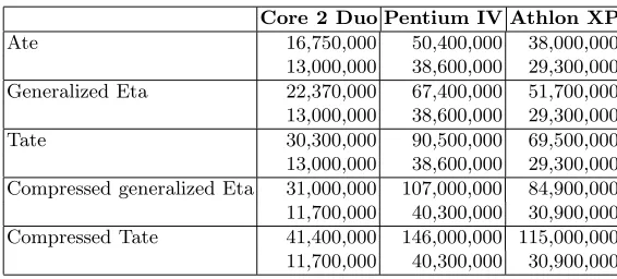
In the Miller loop we entirely avoided to do field inversions, by computing the elliptic curve operations in Jacobian coordinates and by using the compressed representation and storing denominators separately as described in Subsection 5.2. For multiplication and squaring of torus elements we use the algorithms given in Appendix A. The figures in table 2 indicate that, depending on the machine architecture, compressed pairing computation is about 20-45% slower than standard pairing computation, if both computations are optimized for com-putation speed rather than memory usage.
Performance was measured on a 2.2 GHz Intel Core 2 Duo (T7500), a 2.4 GHz Intel Pentium IV (Northwood) and an AMD Athlon XP 2600+ running on 1.9 GHz. The CPU cycles required for Miller loop and final exponentiation respec-tively are given in Table 2.
3
p 82434016654300679721217353503190038836571781811386228921167322412819029493183
n 82434016654300679721217353503190038836284668564296686430114510052556401373769 bitsize 256
t 287113247089542491052812360262628119415
k 12
λc (t−1)8
modn
Table 1.Parameters of the curve used in our implementation
Core 2 Duo Pentium IV Athlon XP
Ate 16,750,000 50,400,000 38,000,000
13,000,000 38,600,000 29,300,000 Generalized Eta 22,370,000 67,400,000 51,700,000 13,000,000 38,600,000 29,300,000
Tate 30,300,000 90,500,000 69,500,000
13,000,000 38,600,000 29,300,000 Compressed generalized Eta 31,000,000 107,000,000 84,900,000 11,700,000 40,300,000 30,900,000 Compressed Tate 41,400,000 146,000,000 115,000,000 11,700,000 40,300,000 30,900,000
Table 2.Rounded average results of measurements on various CPUs. The upper num-ber describes cycles needed for the Miller loop, the lower numnum-ber cycles needed for final exponentiation
7
Conclusion
We have described explicit formulæ for pairing computation in compressed form for the Tate and Eta pairings. For different AES security levels we have also indicated families of curves amenable to pairing compression where generalized versions of the Eta and Ate pairings are very efficient. Our implementations and cost measurements show that the pairing algorithms in compressed form are on certain platforms only about 20% slower than the conventional algorithms. The algorithms in compressed form have the advantage that they can be implemented without finite field inversions. This is not only an advantage for pairing com-putations on restricted devices, but also favors implementation of inversion-free windowing methods for the Miller loop. Furthermore compressed pairing com-putation gives more flexibility in trading off comcom-putation speed versus memory requirement.
Acknowledgments
We thank the anonymous referees and are grateful to Tanja Lange, Mike Scott, Steven Galbraith and Rob Granger for their valuable comments on earlier ver-sions of this work. The first and third authors did portions of this work at the Institute for Theoretical Information Technology, RWTH Aachen University.
References
1. P. S. L. M. Barreto, S. D. Galbraith, C. ´O’ h´Eigeartaigh, and M. Scott. Effi-cient pairing computation on supersingular abelian varieties. Designs, Codes and Cryptography, 42(3):239–271, 2007.
2. P. S. L. M. Barreto and M. Naehrig. Pairing-friendly elliptic curves of prime order. InSelected Areas in Cryptography – SAC’2005, volume 3897 ofLecture Notes in Computer Science, pages 319–331. Springer-Verlag, 2006.
3. A. J. Devegili, C. ´O h´Eigeartaigh, M. Scott, and R. Dahab. Multiplication and squaring on pairing-friendly fields. Cryptology ePrint Archive, Report 2006/471, 2006. http://eprint.iacr.org/.
4. A. J. Devegili, M. Scott, and R. Dahab. Implementing cryptographic pairings over barreto-naehrig curves. Cryptology ePrint Archive, Report 2007/390, 2007. Available fromhttp://eprint.iacr.org/2007/390.
5. C. Doche. Finite field arithmetic. In H. Cohen and G. Frey, editors, Handbook of Elliptic and Hyperelliptic Curve Cryptography, chapter 11, pages 201–238. CRC Press, 2005.
6. D. Freeman, M. Scott, and E. Teske. A taxonomy of pairing-friendly ellip-tic curves. Cryptology ePrint Archive, Report 2006/372, 2006. Available from
http://eprint.iacr.org/2006/372.
7. R. Granger, D. Page, and M. Stam. On small characteristic algebraic tori in pairing based cryptography. LMS Journal of Computation and Mathematics, 9:64–85, March 2006.
8. F. Hess, N. Smart, and F. Vercauteren. The eta pairing revisited. IEEE Transac-tions on Information Theory, 52(10):4595–4602, October 2006.
9. E. J. Kachisa, E. F. Schaefer, and M. Scott. Constructing brezing-weng pairing friendly elliptic curves using elements in the cyclotomic field. Cryptology ePrint Archive, Report 2007/452, 2007. http://eprint.iacr.org/.
10. E. Lee, H. Lee, and C. Park. Efficient and generalized pairing computation on abelian varieties. Cryptology ePrint Archive, Report 2008/040, 2008. http:// eprint.iacr.org/.
11. S. Matsuda, N. Kanayama, F. Hess, and E. Okamoto. Optimised versions of the ate and twisted ate pairings. In Steven D. Galbraith, editor,IMA Int. Conf., volume 4887 ofLecture Notes in Computer Science, pages 302–312. Springer, 2007. 12. K. Rubin and A. Silverberg. Torus-based cryptography. InAdvances in Cryptology
– Crypto’2003, volume 2729 ofLecture Notes in Computer Science, pages 349–365. Springer-Verlag, 2003.
13. M. Scott and P. S. L. M. Barreto. Compressed pairings. InAdvances in Cryptology – Crypto’2004, volume 3152 ofLecture Notes in Computer Science, pages 140–156, Santa Barbara, USA, 2004. Springer-Verlag.
15. C. Zhao, F. Zhang, and J. Huang. A note on the ate pairing. Cryptology ePrint Archive, Report 2007/247, 2007. Available fromhttp://eprint.iacr.org/2007/ 247.
A
Compressed multiplication and squaring algorithms
Algorithm 1Squaring of the element (A0, A1, A)
Require: (A0, A1, A)∈Fp2×Fp2\ {0} ×Fp
Ensure: (C0, C1, C) = (A0, A1, A)2 r1←A2
0,r2←A0r1,S0←r1r2,t0←A 2
,r4←r2t0,r5←A2
1,r5←A1r5,
r3←r1r5,r4←r4−r3,r0←r4ξ,r0←2r0,S1←S0+r0,r4←r4−r3,r4←r4ξ,
S0 ←S0+r4,t1←t2
0,r4←t1A0,r0← 1
3r4,r1←r5t0,r0←r0−r1,r1←2r1, r4←r4−r1,r0←ξ2
r0,r4←ξ2
r4,S0←S0+r0,S0←S0A0,S1←S1+r4,
S1 ←S1A0,r2←r2
5,r2←r2ξ 2
,r4←t1t0,r4← 1 27ξ
3
r4,r1←r2+r4,S0←S0+r1,
S←S0A,S0←S0A0,S←2S,r4←4r4,r1←r2+r4,S1←S1+r1,S1 ←S1A1,
r1←r5t1,r1← 1 3ξ
3
r1,S0←S0−r1
WriteS=s0+is1
r1←(s0−is1),C0←S0r1,C1←S1r1,C←Sr1=s2 0+cs
2 1
return(C0, C1, C)
Algorithm 2Multiplication of elements (A0, A1, A) and (B0, B1, B)
Require: (A0, A1, A),(B0, B1, B)∈Fp2×Fp2\ {0} ×Fp
Ensure: (C0, C1, C) = (A0, A1, A)·(B0, B1, B)
R0 ←A2
0,t1←A 2
,r3← 1
3ξt1,R0←R0+r3, R1 ←B2
0,t1←B 2
,r3←1
3ξt1,R1←R1+r3
r3←A1B1,r4←A0B0,t1 ←AB,r5←t1ξ,r4←r4+r5,S0←r3r4,S2←r2 3 S2 ←S2ξ,r4←A0B1,r5←A1B0,r4←r4+r5,r6←r3ξ,S1←r6r4,r4←R0R1 S1 ←S1+r4,r4←A1R1,r5←r4A0,S2←S2+r5,T2 ←r4A,r4←r4A1,
S0 ←S0+r4,r4←B1R0,r5←r4B,T2←T2+r5,r5←r4B0,S2←S2+r5,
r4←r4B1,S0←S0+r4,S0←S0ξ,T0←A0B,r4←B0A,T0←T0+r4,T0←r6T0,
T1←A1B,r4←B1A,T1←T1+r4,T1 ←T1r6
r0←T2
0,r1←T 2
1,r2 ←T 2
2,T ←r0T0,r3←r1T1,r3←r3ξ,T ←T+r3 r3←r2T2,r3 ←r3ξ2
,T ←T+r3,r3←T1T2,r3←r3ξ,U0←r0−r3,r3←r3T0 r3←3r3,T ←T−r3,r3←T0T1,U1 ←r2ξ,U1←U1−r3,r3←T0T2,U2←r1−r3 V0←S0U0,r0←S1U2,r1←S2U1,r0←r0+r1,r0←r0ξ,V0←V0+r0
V1←S0U1,r0←S1U0,V1←V1+r0,r0←S2U2,r0←r0ξ,V1 ←V1r0
WriteT =t0+it1
r1←(t0−it1),C0←V0r1,C1←V1r1,C←Sr1=t2 0+ct
2 1