Division VII
SEISMIC FRAGILITY CURVE ESTIMATION USING SIGNALS
GENERATED WITH GMPE -
CASE STUDY ON THE KASHIWAZAKI-KARIWA POWER PLANT
Fan WANG1, Cyril FEAU1
1 Research Engineers, CEA, DEN, DANS, DM2S, SEMT, EMSI Laboratory, F-91191 Gif-sur-Yvette,
France
ABSTRACT
As one of the participants to the international KARISMA Benchmark, we had conducted soil-structure interaction analysis on the Unit 7 reactor building of the Kashiwazaki-Kariwa nuclear power plant (Japan) using a full 3D finite element model. In this paper, we focused on the uncertainty propagation through the soil-structure system. For this purpose, a simplified model representing the largely embedded reactor building has been used for computation efficiency as a large number of numerical simulations were necessary.
Seismic signals generated with NGA GMPE according to the July 2007 NCO earthquake scenario have been used to estimate the fragility curves. In the process, soil non-linearity caused by each seismic signal has been taken into account using the equivalent linear method. The results suggest that defining the control point of the input motion at the soil surface as prescribed in the French nuclear practice is not appropriate and may lead to biased results when performing non-linear soil-structure fragility analysis. The control point should be defined at the “outcropping bedrock” level.
INTRODUCTION
Following the 16 July 2007 Niigataken-Chuetsu-Oki (NCO) earthquake in Japan which affected severely the Kashiwazaki-Kariwa Nuclear Power Plant located just 16 km from the epicentre, the International Atomic Energy Agency (IAEA), launched the KARISMA benchmark (KAshiwazaki-Kariwa Research Initiative for Seismic Margin Assessment) (IAEA, 2011 and 2013). The objective was to find out if current simulation methodologies used by different member states were able to capture the main features of the seismic response under strong Soil-Structure Interaction (SSI). As one of the participant to the benchmark, we have conducted seismic soil-structure interaction analysis in which the Unit 7 reactor building and the surrounding soil were modelled by full 3D finite elements and the far-field soil by viscous absorbing boundaries (Wang and Rambach, 2013).
In this paper, we focus on the uncertainty propagation through the soil-structure system of Unit 7 reactor building with the objective to estimate the fragility curve of some selected plant equipment due to the variability of the input seismic signals. This work is a part of the ongoing French research project SINAPS@ (Earthquake and Nuclear Installations: Ensuring and Sustaining Safety) which aims to explore the uncertainties in databases, knowledge of the physical processes and methods used at each step of the evaluation of the seismic hazard and the vulnerability of structures and equipment (Berge-Thierry, 2017).
by the cumulative distribution of a lognormal random variable, of an equipment associated with ground-motion variability. The parameters of the curve (median and standard deviation) are evaluated using the principle of maximum likelihood. In the process, soil non-linearity caused by each seismic signal is taken into account using the equivalent linear method through soil column deconvolution.
STRUCTURE MODELS
KARISMA Benchmark Experience
During KARISMA benchmark (2009-2013) we conducted full 3D finite element modelling for the structure and the nearby soil using the code CAST3M developed by the CEA (website: http://www-cast3m.cea.fr). The model (see Figure 1) was composed of about 150 000 finite elements and the far-field soil which extends to infinity (lateral sides and bottom) was represented by viscous absorbing boundaries (Lysmer and Kuhlemeyer, 1969).
Figure 1. Full 3D finite element modelling of the reactor building and the near field soil used for KARISMA benchmark (Wang and Rambach, 2013)
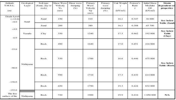
Table 1: Soil properties near Unit 7 reactor building (IAEA, 2011)
Attitude T.M.S.L. (m) Geological Layer Soil type (Sand, clay or
rock) Shear Wave Velocity Vs (m/s) Shear wave damping (%) Primary Wave Velocity Vp (m/s) Primary wave damping (%) Unit Weight g (kN/m3) Poisson’s Ratio n Initial Shear Modulus G0 (kN/m2) Strain dependent soil properties +8.0 Nishiyama
Property of soil (NCOE) - RB7
Rock Rock 16.1 0.347 +4.0 Yasuda Sand 150 Sand Sand Grade Level (+12.0) Clay 65 700
200 16.1 0.308
192 000 330 See below Table (Clay) -6.0 Nishiyama
490 17.0 0.451 416 000
-136.0
The free
surface of the Rock Rock 650 -155.0 720 -33.0 530 590 Rock -90.0 310 380 1240 1640 1700 1710 1790 36 000 See below Table (Sand) 17.3 0.462
1900 1 050 000
0.424 832 000
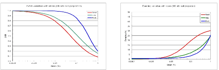
Figure 2.Strain dependent shear modulus and damping ratio of the soil near Unit 7 reactor building (IAEA, 2011)
The properties of soil layers are given in Table 1. Strain-dependant shear modulus (G/G0) and damping ratio for sand, clay and rock layers which constitute the soil profile are plotted in Figure 2 which allowed to take into account soil non-linearity caused by the earthquake in a linear equivalent way. The principal lateral-resisting members of the structure, i.e. the exterior walls and the Reinforced Concrete Containment Vessel (RCCV), were assigned non-linear constitutive laws in case they exhibit non-linear behaviours.
Time domain integration was carried out directly on the coupled soil-structure system. The analysis has given good results compared to the recorded in-structure response during NCO earthquake (Wang and Rambach, 2013). The benchmark experience has led to some very important guidelines for our current study:
The reactor building remained linear elastic for the NCO earthquake in the full 3D FEM analysis despite the very strong surface motion recorded on the site (PGA = 1.22g E-W) and this is consistent with the post-earthquake observations that no significant concrete cracking were seen on the building. Consequently, we can use an elastic model for the reactor building provided that the input seismic signals are not significantly stronger than the recorded NCOE in terms of PGA level.
Soil non-linearity was very strong as the linear equivalent soil model obtained by the benchmark organizer through soil column deconvolution showed shear modulus reductions greater than 90% near the ground surface. The largest shear strain of the soil column was actually 0.72% which is largely beyond the commonly admitted limit of 0.1% soil strain (ASN, 2006) and yet the numerical results based on this model were in good agreement with the recorded in-structure responses. We think it is reasonable to restraint the maximum soil strain to 0.8% in our study. This means that all input signals which create soil strain beyond this threshold will be eliminated from the simulation. We can thus expect that the input signals used in the simulations will not exceed significantly the site-recorded motions in terms of intensity.
Simplified Model Used in the Current Study
The need to simplify the system model concerns the building structure as well as the foundation soil. To make the modeling representative, it is necessary to take into account the large embedment of the building and the flexibility of the soil-building interface. These two features of the benchmark reactor building can play important roles in the soil-structure interaction but do not exist or are often considered negligible for the nuclear power plants built in France.
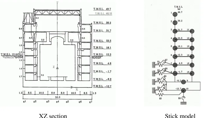
A lumped-mass stick model (Figure 3 below) for the reactor building, used by TEPCO(IAEA, 2011), the owner of the power plant has been adopted and implemented in the Code CAST3M (website: http://www-cast3m.cea.fr) for the current work. This is a very simple finite element model but it can describe the two main features of the building mentioned above.
XZ section Stick model
Figure 3. XZ cross section of the reactor building (left) and lumped-mass stick model for X direction (right) (IAEA, 2011)
The stick model is composed of two vertical beams connected by rigid horizontal links at each floor and founded on the basemat. According to the geometry of the structure, two models with slightly different characteristics are used: one for the NS (XZ plan, Figure 3) direction and the other for the EW (XY plan, not presented here) direction. The representation of the building by these stick models implies two perpendicular symmetry planes which is not perfectly the case here (a small eccentricity was found during the benchmark). The analyses will be performed respectively in the X and Y direction and combined if necessary, while the vertical motion and the torsion of the building will not be considered in this study.
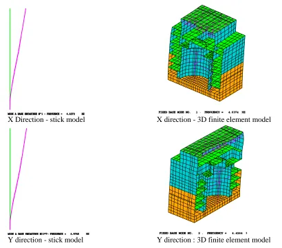
X Direction - stick model X direction - 3D finite element model
Y direction - stick model Y direction : 3D finite element model
Figure 4. Comparison of the first fixed-base mode in the X and Y directions, between lumped-mass stick and 3D finite element models
The foundation soil is represented by their dynamic impedance functions which are schematised by soil springs K1 to K10 as shown in Figure 3.No coupling is supposed between these springs. Springs K1, K2, K3, K4 and K7, K8, K9, K10 respectively for translational and rocking motions are the so-called Novak’s “side springs”. They are calculated for each soil layer as the impedances of a rigid massless cylindrical foundation in an elastic plane-strain infinite medium (Novak et al, 1978). Because of the potential separation between the wall and the soil near the ground surface, the first layers of soil to a depth of 6 meters are not considered in the calculation of the soil springs according to ASCE Standard 4-16 (SEI, 2017).
K5 and K6 are the so-called “bottom soil springs” which are the impedances of a rigid massless disk resting on the surface of semi-infinite elastic medium considering only soil layers beneath the foundation. These functions can be found in impedance handbooks such as Sieffert and Cevear (1992). The shape of the building being rectangular, equivalent circular foundations are used to determine the soil springs. The equivalent radius are calculated on the equivalence of surface for the translational spring and equivalence of moment of inertia for rocking spring.
be used to calculate the impedance of each soil layer. The soil beneath the foundation will be replaced by an equivalent homogeneous medium to determine the bottom soil springs.
SEISMIC SIGNALS
Ground Motion Prediction Equation (GMPE)
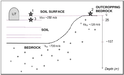
Synthetic seismic signals were produced using the Campbell and Bozorgnia (2008) empirical Ground Motion Prediction Equation (GMPE) and considering the NCOE 2007 scenario (Mw = 6.6 and epicentral distance of 16 km). Two approaches were employed in the process: in the first one, signals were generated for the soil surface (top of grade) while in the second one, they were generated for a virtual outcropping bedrock.
Figure 5. Simplified scheme of reactor building which is embedded over 25 m. Bedrock is found at ~167 m in depth. Stars indicate location of different “control points” (extract from Berge-Thierry 2017).
Approach 1: Soil Surface Signals
In this approach, seismic signals were specified for the control point 1 as shown in Figure 5 on the ground surface with the real soil condition of the reactor building site (Vs30 = 250 m/s). This approach correspond
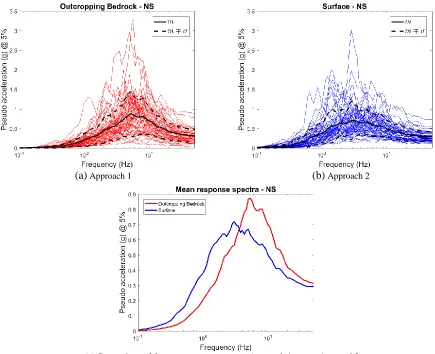
to the usual French engineering practice recommended by the French nuclear safety authority. As a matter of fact, in France the reference seismic input has always been defined on the surface of the free field soil (ASN, 2006). A set of 50 synthetic ground motions was generated initially (Zentner, 2014) whose mean response spectrum fits the target NCOE 2007 scenario spectrum on a soft soil site. To increase the seismic inputs number, and to cover a large range of strong motions, the “classical engineering scaling” process is applied on the signal set with amplification factors of 0.5, 1, 2, 2.5 and 3. The response spectra of initial 50 surface signals are shown in Figure 6(a).
Approach 2: Outcropping Bedrock Signals
In this second approach, seismic signals were specified for the control point 2 on the outcropping bedrock with a rock site conditions (Vs30 = 720 m/s) as shown in Figure 5. This approach is not the current French
practice but was adopted in this study because it is probably more relevant considering the effect of the high soil non-linearity on the site. This effect cannot be precisely predicted by the Campbell and Bozorgnia empirical equation which is not site-specific by nature. As in approach 1, a set of 50 synthetic ground motions was generated whose mean response spectrum fits the target NCOE 2007 scenario spectrum on a rock site. The same scaling process was applied with factors of 0.5, 1, 2, 2.5 and 3 as previously. Figure
OUTCROPPING BEDROCK SOIL SURFACE
SOIL
6(b) shows the spectra of the initial 50 outcropping signals. For the sake of comparison, the mean spectra for the signals of two approaches are plotted in Figure 6(c) which shows that the peak of spectra of the soil surface signals is lower than that of a rock site.
(a) Approach 1 (b) Approach 2
(c) Comparison of the mean response spectra Approach 1 versus Approach2
Figure 6. Synthetic signal response spectra for 5% damping: (a) on the soil surface, (b) on the outcropping bedrock. Curves are the means and dotted curves are the means (+/-) one standard deviation.
SOIL COLUMN DECONVOLUTION
By assuming the soil near the reactor building horizontally stratified, soil column deconvolution has been carried out for each synthetic signal by supposing that the seismic waves propagates vertically. This was done on a vertical column of soil representative of the site. The goal was twofold: the first was to obtain the linear equivalent soil profile to calculate the soil springs and the second was to get the ground motions at different depths of the free field, especially the motion at the structure foundation level which is used as the “foundation input motion” to compute the response of the coupled soil-structure system.
Computer Codes Used
Both codes are based on the same assumptions of one-dimensional wave propagation on a vertical soil column and an iterative process using the strain-dependent soil properties curves of Figure 2 as mentioned above but their methods of computation are different.
In CAST3M, the deconvolution is performed numerically in the time domain. The soil column is explicitly represented by solid finite elements which are constrained in the vertical direction. A horizontal impulsive force is applied at the bottom of the column and the dynamic response of every node are computed in the time domain. In doing this, a Rayleigh damping model has to be used which means the damping ratio is frequency-dependent. Transfer functions of the soil column are obtained by transforming the computed responses to the frequency domain.
On the other hand, the code EERA is a modern implementation of the code SHAKE in which the deconvolution is performed analytically in the frequency domain with a constant frequency-independent damping ratio.
Signal Deconvolution and Limit of Validity
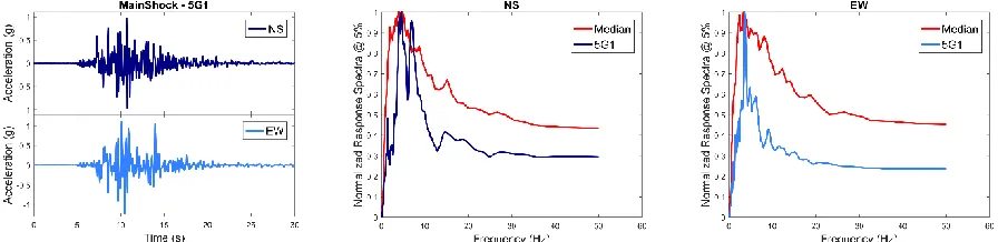
The signals for Approach 1 were generated for the soils surface (control point 1). Each of the 250 signals (amplification factors of 0.5, 1, 2, 2.5 and 3 on initial 50 data) has been de-convoluted to different soil depths using both computer codes described above. In this process, the frequency content over 15 Hz was filtered out because the GMPE response spectrum used tends to be wide band which doesn’t reflect the reality of the site as can be seen in Figure 7 showing the free-field recordings during the NCOE main-shock.
Figure 7. Recorded horizontal accelerations during the 2007 NCO earthquake (Station 5G1, free field surface near RB7) and their normalized response spectra (blue curves) versus the normalized medians of
the synthetic ground motions response spectra for 5% damping (red curves)
The signals for Approach 2 were generated for outcropping bedrock (control point 2). Each of the 250 signals (amplification factors of 0.5, 1, 2, 2.5 and 3 on initial 50 data) has also been de-convoluted to different soil depths using both computer codes but this time they have not been filtered as previously.
A significant number of seismic signals (notably those scaled with strong amplifying factors 2, 2.5 and 3, and more particularly among the Approach 1 signals) produced “divergence” in the deconvolution process, highlighting the problem related to the use of the linear equivalent method beyond its usual limitations (0.1% for maximum shear strain in the literature, threshold also recommended by ASN (2006)) to a soil site which is highly non-linear under strong seismic motions. In the following, all signals which lead to soil shear strain exceeding 0.8% will in fact be eliminated from the simulation population as it has been mentioned earlier in this paper.
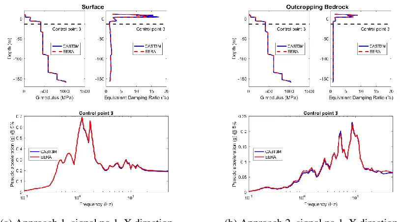
We can see that the two codes lead to almost the same results except for some small differences on the response spectra which are due to the different damping models used by the two codes.
(a) Approach 1, signal no.1, X direction (b) Approach 2, signal no.1, X direction
Figure 8. Soil column deconvolution: CAST3M vs EERA, linear equivalent soil profiles and response spectra at -13.7 m TMSL (bottom face of the basemat).
REACTOR BUILDING RESPONSE
Foundation Input Motion
In order to calculate the reactor building response, the free field motion obtained by deconvolution at the depth corresponding to the bottom face of the basemat (-13.7m TMSL, Figure 3) has been taken as the “foundation input motion”. This is an approximation often used in the practice which simplifies enormously the computation of building response. The real “foundation input motion” should be the kinematic response of the soil-structure system (soil + massless structure) under the seismic motion.
Response of the Building
FRAGILITY CURVES ASSESSMENT
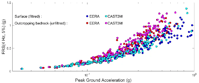
In this study, fragility curves are estimated for a single-mode equipment at 4 Hz damped at 5% fixed on the third floor (+23.5 m TMSL). Thus, the failure criterion is the exceedance of the Floor Response Spectra at 4 Hz (FRS (4 Hz, 5%)) of a level of acceleration which will be considered as a variable to be more comprehensive. Figure 9 shows the scatter plots of the maxima of the responses of the equipment subjected to the four sets of foundation input motions (two deconvolution codes and two approaches for generation seismic signals), as function of PGA values estimated at the control point 3. This figure shows that the results produced by the four sets of data (for which the soil shear strain is lower or equal to 0.8%) seem to have a similar trend, and are particularly coherent in the very low range of PGA.
Figure 9. Floor Response Spectra at 4 Hz versus PGA values evaluated at the control point 3 – comparison between the results of CAST3M and EERA for the two approaches
The fragility curves have been approximated by the cumulative distribution function (cdf) of a lognormal random variable:
𝑃𝑓(𝑎) = Φ (ln(𝑎 𝐴𝛽⁄ 𝑚))
where Φ(∙) is the standard Gaussian cdf. The median 𝐴𝑚 and the standard deviation 𝛽 have been evaluated using the principle of maximum likelihood and a confidence interval has been estimated using a bootstrap method (Zentner, 2010).
a b
Figure 10. Two examples of median fragility curves and their 95% confidence intervals for a single-mode equipment at 4 Hz damped at 5%, for failure criteria equal to: (a) 0.2g and (b) 0.7g.
To be more comprehensive, Figure 11 shows, for a large range of failure criteria (from 0.2g to 1.1g) both the influence of the deconvolution code and of the control point to define the initial seismic motions (before deconvolution) on the estimated fragility curves parameters, through their median values and their 25% and 75% quantiles (represented by the bottom and the top of the box of each estimation). Figure 11 clearly shows that only at very low acceleration levels (i.e. for which the soil distortion is of an order of magnitude of 0.1% or less) the two approaches are coherent, but when loading increases, the results obtained with the seismic motions defined at the surface, strongly differ from those obtained with the seismic motions defined at the outcropping bedrock. These trends are similar for both codes, although with CAST3M the medians of the fragility curves are slightly lower than those obtained with EERA due to the difference of the damping model.
(b)
Figure 11. Comparison between estimations of the fragility curves parameters obtained with the four sets of data: (a) 𝐴𝑚 and (b) 𝛽 versus failure criteria. Circles are for median values
computed with 200 bootstrap samples, vertical lines show the dispersion of the samples, the bottom and the top of the boxes indicate the quantiles at 25% and 75%.
This study illustrates the biases which can be introduced into the fragility assessment process of a complex study treated here with simple and practical numerical models. To be more comprehensive, the next part of this paper proposes a discussion aimed at giving a better understanding of these results.
DISCUSSION
In this part, all the results have been obtained with the EERA deconvolution code, since the numerical results of CAST3M and EERA are very similar.
Uncertainty propagation
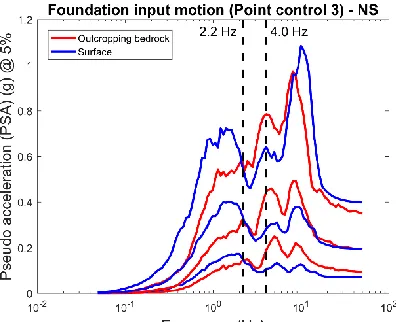
The previous results (see Figure 11) show that the two approaches appear to be globally coherent for low excitation levels (i.e. for low failure criteria). However, for the signals calculated at the control point 3 in the NS direction for example, Figure 12 shows significant differences in the median spectra, expressed in pseudo acceleration for a damping ratio of 5%, as well as in their quantiles at 15% and 85%.
Figure 12. Comparison of the medians and the quantiles at 15% and 85% of pseudo acceleration response spectra of signals calculated at the control point 3 in the NS direction with
To understand the discrepancies between these results (Figure 11 and Figure 12), it is necessary to have in mind that: (i) the variabilities of the coefficients 𝐺 which are used to determine the bottom soil springs are very small since their coefficient of variation (cov) are less than 3%, as shown in Figure 13(a). Indeed, in this problem, important variabilities are concentrated in the upper soil layers which have very non-linear behavior; (ii) in the SSI model considered in this study, the linear dependence between 𝐺 and the bottom soil springs implies that the cov of these springs are very small, as shown in figure 13(b); (iii) in the model of the coupled soil-structure system, the bottom soil springs’ contribution to the overall rigidity is dominant. Figure 13(c) illustrates this point by showing the contribution of the mean generalized stiffnesses of the building 𝐸[𝐾𝑔𝑏1 ] and the springs 𝐸[𝐾𝑔𝑘𝑖1 ], 𝑖 ∈ [1,10], to the mean generalized stiffness 𝐸[𝐾𝑔1] = 𝐸[𝐾𝑔𝑏1 ] +
∑10𝑖=1𝐸[𝐾𝑔𝑘𝑖1 ] of the first eigenmode of the coupled system.
(a) (b)
(c) (d)
Figure 13. Comparison between the two approaches: (a) cov of G vs depth, (b) cov of springs’ values, (c) springs’ contributions to the generalized stiffness of the coupled system and (d) cov of the
springs’ generalized stiffnesses
show that the generalized mass 𝑀𝑔1 of the first eigenmode of the coupled system (and by extension its
effective mass) is quasi-deterministic since its cov is of an order of magnitude of 0.5%, thus:
𝑐𝑜𝑣(𝑓1) = 𝑐𝑜𝑣(𝜔1) < 𝑐𝑜𝑣(𝜔12) ≃ 𝑐𝑜𝑣(𝐾𝑔1) = 𝑐𝑜𝑣(𝐾𝑔𝑏1 + ∑ 𝐾𝑔𝑘𝑖1 10
𝑖=1
)
where 𝑓1, 𝜔1 and 𝐾𝑔1 are respectively the frequency, the circular frequency and the generalized stiffness of
the first eigenmode of the coupled system. Assuming that the generalized stiffnesses of the building and springs can be considered as independent random variables (which is not really true), and considering the group of the variables associated to the bottom soil springs (springs 5 and 6), whose the generalized stiffness is noted 𝐾𝑔𝑘561 , it follows :
𝑐𝑜𝑣(𝐾𝑔1) ≃
√𝑉(𝐾𝑔𝑏1 ) + ∑ 𝑉(𝐾 𝑔𝑘𝑖1 ) 10
𝑖=1
𝐸[𝐾𝑔𝑏1 ] + ∑ 𝐸[𝐾 𝑔𝑘𝑖1 ] 10
𝑖=1
≃𝜎(𝐾𝑔𝑘56
1 )√10
𝐸[𝐾𝑔𝑘561 ] ≃ 3𝑐𝑜𝑣(𝐾𝑔𝑘561 ) ≃ 3 × 3.510−3≃ 10−2
since 𝐸[𝐾𝑔𝑘561 ] ≫ 𝐸[𝐾𝑔𝑏1 ] and [𝐾𝑔𝑘𝑖1 ] 𝑖 ∈ [1,4] ∪ [7,10] and the variances are of the same order of
magnitude. Consequently, in this case study, the variability of the response of the equipment is mainly due to the variability of the signals calculated at the control point 3.
Empirical sensitivity analysis
The previous results make it possible to carry out an empirical sensitivity analysis considering a simplified SSI model composed of a one dof linear system strongly damped subjected to single direction of excitation. Thus, in the NS direction for example, it can be noticed in Figure 14 that at 4Hz the differences between the spectra are smaller at the floor level than at the control point 3, which implies a reduction of the gaps between the two approaches, especially at low levels of excitation.
Figure 14. Comparison of the medians and the quantiles at 15% and 85% of floor response spectra of signals calculated at the control point 3 in the NS direction for the two approaches with
the simplified SSI model
responses of the equipment. Consequently, medians of fragility curves are more important for an equipment placed in the building than at the ground level. Moreover, the effect of the coupled system tends to reduce the gaps between the two approaches for the low failure criteria and to increase them for the high failure criteria. The values of the logarithmic standard deviations are comparable between the two approaches.
(a) (b)
(c) (d)
Figure 15. Comparison between the two approaches with a simplified SSI model whose frequency correspond to the first eigenmode frequency of the coupled system which is equal to 2.2 Hz: (a) PSA (4
Hz, 5%) vs PGA, (b) FRS (4 Hz, 5%) vs PGA, (c) 𝐴𝑚 vs failure criterion and (d) 𝛽 vs failure criterion
(a) (b)
(c) (d)
Figure 16. Results of an empirical sensitivity analysis with simplified SSI models: (a)-(b) 𝐴𝑚 and
𝛽 vs equipment frequency for three failure criteria in the case of a simplified coupled system at 2.2 Hz; (c)-(d) 𝐴𝑚 and 𝛽 vs equipment frequency for three failure criteria in the case of a simplified coupled
system at 3.5 Hz
These figures show similar trends to those observed in the main study, namely that the approach for which the excitation is defined at the surface tends to quasi-systematically underestimate the risk of failure.
CONCLUSION
approach for which the excitation is defined at the surface tends to quasi-systematically underestimate the risk of failure. To avoid this and knowing that in the non-linear case, the deconvolution problem is mathematically ill-posed, the control point should be defined at the outcropping bedrock level. This study also illustrates the necessity to control uncertainties in seismic loading (the coherency between the GMPE defined at the surface or at the outcropping bedrock for example), to have a better understanding of the observed results. Finally, it is worth noting that the results obtained in this study was based on a simplified modeling of the soil-structure system and on the linear equivalent method for soil column deconvolution, and should be confirmed by comparison with results of more sophisticated models.
ACKNOWLEDGEMENTS
Special thanks to Zentner I. (EDF France) for generating the synthetic seismic signals used in this study.
REFERENCES
SEI (2017) “ASCE Standard ASCE/SEI 4-16: Seismic analysis of safety related nuclear structures” American Society of Civil Engineers (ASCE)
ASN (2006) “Guide/ASN/2/01, Prise en compte du risque sismique à la conception des ouvrages de génie civil des installations nucléaires de base, à l'exception des stockages à long terme des déchets, radioactifs”, French Nuclear Safety Authority
Bardet J.P., Ichii K., And Lineera C.H. (2002): “A Computer Program for Equivalent-linear Earthquake site Response Analyses of Layered Soil Deposits” Department of Civil Engineering, University of Southern California.
Berge-Thierry C., Wang F., Feau C., Zentner I., Voldoire F., Lopez-Caballero F., Le Maoult A., Nicolas M. and RagueneauF. (2017) “The SINAPS@ french research project: first lessons of an integrated seismic risk assessment for nuclear plants safety” 16th World Conference on Earthquake, Santiago Chile.
Campell K.W., Bozorgnia Y. (2008) “NGA ground motion model for the geometric mean horizontal component of PGA, PGV, PGD and 5% damped linear elastic response spectra for periods ranging from 0.01 to 10s” Earthquake Spectra 24:1
IAEA (2011) “KARISMA Benchmark: Guidance document Part 1: K-K unit 7 R/B structure - Phase I, II & III” IAEA-EBP-SS-WA2-KARISMA-SP-002, Rev. 04, Vienna
IAEA (2013) “Review of seismic evaluation methodologies for nuclear power plants based on benchmark exercise” IAEA-TECDOC-1722, Vienna
Lysmer J., Kuhlemeyer RL. (1969) “Finite dynamic model for infinite media” J Eng. Mech. Div. ASCE 95(EM4):859-877
Novak M., Nogami T., Aboul-Ella F. (1978) “Dynamic soil reactions for plane strain case”, Proceeding of ASCE EM4, pp.953-959
Sieffert J-G, Cevear F. (1992) “Manuel des fonctions d’impédance” Ouest Edition Presse Académique
Wang F., Rambach J.M. (2013). “Contribution to the IAEA soil-structure interaction KARISMA benchmark”, Proceedings of the 22nd Conference on Structural Mechanics in Reactor Technology
San Francisco, US.
Zentner I., Allain F., Humbert N. and Caudron M. (2014). “Generation of spectrum compatible ground motion and its use in regulatory and performance-based seismic analysis”. Proceedings of the 9th International Conference on Structural Dynamics, EURODYN. Porto, Portugal.