Xiaoyong Zheng and Ivan Kandilov).
This dissertation consists of two chapters, both of which are lied in empirical analysis of
industry organization topics.
The fist essay proposes a stylized model that elucidates the two channels through which
alternative marketing arrangements (AMAs) can affect the spot market price in livestock
markets. The direct effect of AMAs on spot market price works through their effect on
demand and supply conditions in the spot market. This effect has been widely studied in the
literature. The indirect effect works through their effect on spot market price volatility. This
effect has been ignored in the literature. We then estimate a dynamic (time series) model
with data from the U.S. hog market to test our model implications and quantify the two
effects. We find increases in the use of AMAs increase spot market price volatility and
decrease spot market price level. The short-run effects are small but the long-run effects are
nontrivial.
by
Jong Jin Kim
A dissertation submitted to the Graduate Faculty of
North Carolina State University
in partial fulfillment of the
requirements for the degree of
Doctor of Philosophy
Economics
Raleigh, North Carolina
2012
APPROVED BY:
_______________________________
______________________________
Xiaoyong Zheng
Ivan Kandliov
Committee Co-Chair
Committee Co-Chair
________________________________
________________________________
DEDICATION
BIOGRAPHY
ACKNOWLEDGMENTS
TABLE OF CONTENTS
List of Tables ... vii
List of Figures ... viii
CHAPTER 1 Effects of Alternative Marketing Arrangements on Spot Market Price
Distribution in the U.S. Hog Market ...1
1.1 Introduction ...1
1.2 AMAs in the U.S. Hog Industry ...5
1.3 Data ...7
1.4 Conceptual Framework ...11
1.5 Empirical Strategy and Results ...17
1.5.1 Stationarity Test ...17
1.5.2 GARCH-M Model ...19
1.5.3 Estimation Results ...21
1.5.4 Long-run or Equilibrium Effects of AMAs on Spot Market Price
Distribution ...23
1.6 Conclusions ...25
References ...27
Tables and figures ...32
CHAPTER 2 The Complementarities among Trade Policy Measures: Evidences from
Mexico ...44
2.1 Introduction ...44
2.2 Effect of Trade Liberalization on Firm Productivity ...48
2.2.1 Theories and Empirical Studies ... 48
2.2.2 Complementarities between Trade Policy Measures ...51
2.3.1 Estimating TFP ...54
2.3.2 Testing Complementarities ...56
2.4 Data and Descriptive Analysis ...60
2.4.1 Data ...60
2.4.2 Endogeneity of Trade Policy ...64
2.5 Results ...66
2.5.1 Measuring Productivities ...66
2.5.2 Baseline Results ...67
2.5.3 Robustness Checks ...71
2.5.4 Marginal effects of trade liberalization ...73
2.5.5 Complementarity or Substitutability Test ...76
2.5.6 Cross-Partial Effects between Trade Policy Measures ...78
2.5.7 Complementarities in Two-Digit Industries ...79
2.6 Conclusion ...81
References ...83
Tables and figures ...90
LIST OF TABLES
Table 1.1: Average Daily Transaction Volume (# of Heads in Thousands) ... 33
Table 1.2: Summary Statistics for the Finished Hog Purchase Data ... 34
Table 1.3: Unit Root Test Results ... 35
Table 1.4: GARCH-M Estimation Results: Using Pork CPI as Pork Price ... 36
Table 1.5: GARCH-M Estimation Results: Using Pork Bellies Price as Pork Price ... 37
Table 1.7: Effect of AMAs on Spot Market Price Volatility ... 38
Table 1.8: Effect of AMAs on Spot Market Price Level: Using Pork CPI ... 38
Table 1.9: Effect of AMAs on Spot Market Price Level: Pork Bellies Price ... 38
Table 2.1: Mexico trade liberalization: Trade policy measures and its correlation coefficients (%, June of each year) ... 91
Table 2.2: Descriptive Statistics ... 92
Table 2.3: Initial productivity and changes of trade policies (Cross-Section Estimates) ... 92
Table 2.4: Panel B: Current productivity and subsequent trade policies (Panel Estimates ... 93
Table 2.5: Initial characteristics and the change of trade policies (Political protection ... 93
Table 2.6: Production Function estimations (Proxy: Primary/raw materials) ... 94
Table 2.7: Summary of estimated TPF (Proxy: Primary/raw materials) ... 94
Table 2.8: Impact of trade policy measures on plant productivity ... 95
Table 2.9: Robustness Checks ... 98
Table 2.10: Marginal effects of trade policies on plant level productivity ... 100
Table 2.11: Complementarity test with pair-wise model ... 100
Table 2.12: Complementarity Test with full interaction model ... 101
Table 2.13: Cross-partial Effects of each trade policy measures ... 101
Table 2.13: Heterogeneity of the impacts across 2-digit industries ... 102
LIST OF FIGURES
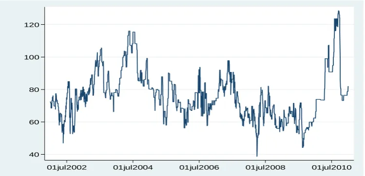
Figure 1.1: Plot of Spot Market Price ... 39
Figure 1.2: Plot of Pork CPI ... 39
Figure 1.3: Plot of the First Difference of Pork CPI ... 40
Figure 1.4: Plot of Pork Bellies Price ... 40
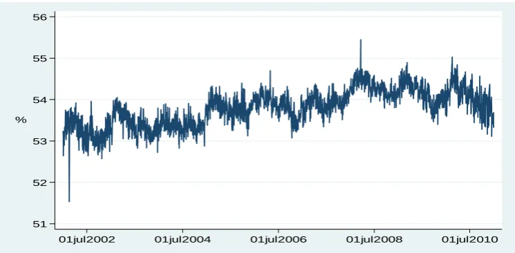
Figure 1.5: Plot of AMA (%) ... 41
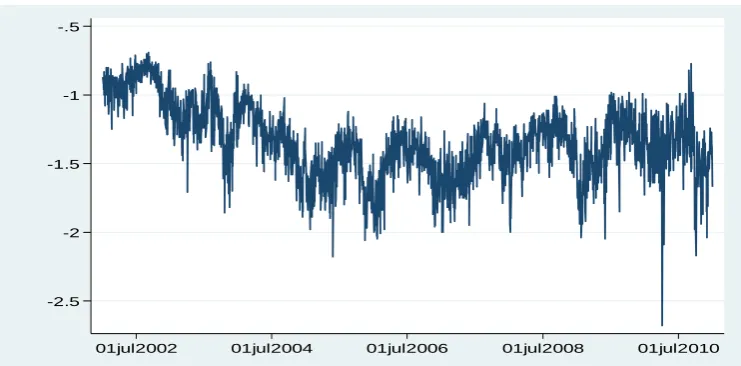
Figure 1.6: Plot of Average Sort Loss ... 41
Figure 1.7: Plot of Average Carcass Weight ... 42
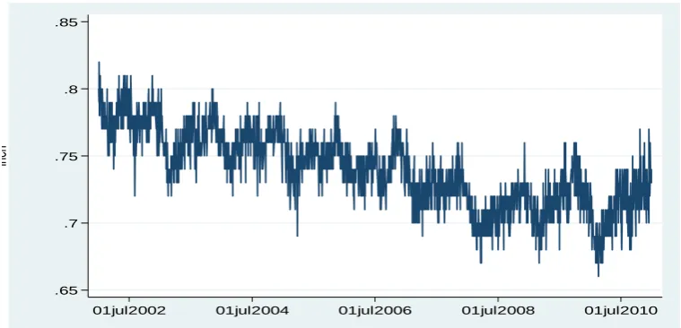
Figure 1.8: Plot of Average Backfat ... 42
Figure 1.9: Plot of Loin Depth ... 43
Figure 1.10: Plot of Average Lean Percent ... 43
CHAPTER 1
Effects of Alternative Marketing Arrangements on
Spot Market Price Distribution in the U.S. Hog
Market
1.1 Introduction
During the past 20 years, one of the most important changes in the U.S. livestock markets is that
packers have relied more and more heavily on alternative marketing arrangements (AMAs) to satisfy
their slaughter needs. As a result, the share of transactions conducted on the spot market has
decreased. For example, in 1999, 36% of the market hogs were transacted on the cash/spot market
(Grimes and Plain, 2009). By the 2004-2005 period, this share had decreased to 24% (Vukina et al.
2007) and our data, which will be detailed below in Section 3, shows that by 2010, this share had
further decreased to only 5.2%.
AMAs in livestock markets mainly take the form of marketing contracts and production contracts.
The main characteristic of both of them, as well as their main difference from the spot market, is that
animals are committed to buyers long before they are finished for slaughter. As we know,
innovations improve social welfare. Just like the introduction of a new good increases the total
welfare of producers and consumers, the emergence of new marketing channels also improve the
welfare of packers and farmers as a whole. This is confirmed by a recent study by Wohlgenant
(2010), who shows that banning the use of AMAs in the hog industry would decrease social welfare.
But the welfare effects of innovations on different groups of economic agents can be quite different.
livestock markets, it is generally believed that AMAs benefit packers and those farmers who contract
with packers for two reasons. First, they are the users of AMAs. If they didn’t benefit from using
these new marketing channels, they would not use them at the first place. Indeed, Key and McBride
(2003) show one of the main reasons for AMAs to become popular is packers can reduce transaction
costs by contracting with fewer and larger producers. Second, since the animals are committed to
buyers well in advance, AMAs help buyers and sellers minimize, or in some cases eliminate, the price
and marketing access risks they usually face when they trade in the spot market. Zheng, Vukina and
Shin (2008) find that more risk-averse farmers are more likely to contract with packers and Franken,
Pennings, and Garcia (2009) find both risk preferences and transactions costs are key determinants of
a packer’s decision in choosing market arrangements.
On the other hand, economists do not agree on the effects of AMAs on the spot market. Some
argue that AMAs remove a large percentage of demand away from the spot market and if the supply
adjusts slowly, there will be a surplus on the spot market and the price will go down (Schroeder et al.
1993). Others argue that AMAs decrease both the demand and the supply to the spot market and
hence the resulting effect on price will be minimal (USDA-AMS 1996). Hence, examining the
effects of AMAs on the spot market is an empirical question. Many studies have been devoted to
study this question. One strand of literature focuses on analyzing the effect of AMAs on spot market
price level. Most of these studies use data from the U.S. fed cattle market and find AMAs either have
a mild negative or an ambiguous effect on the spot market price level (e.g. Elam 1992; Hayenga and
O’Brien 1992; Schroeder et al. 1993; Ward, Koontz and Schroeder 1998; Schroeter and Azzam 2003).
Another strand of literature studies the impact of AMAs on price volatility. For example, Hayenga
and O’Brien (1992) find little evidence that AMAs decrease spot market price volatility. Also, using
between a packer and a feeder in the fed cattle industry increases both the spot market price level and
volatility.
Though studies in the literature have examined the effects of AMAs on spot market price level and
volatility separately, to the best of our knowledge, no study has identified and studied the second
channel through which AMAs influence the spot market price level. The direct effect of AMAs on
spot market price level works through their effects on the demand and supply conditions in the spot
market. The indirect effect, on the other hand, works through their effect on spot market price
volatility. Economic theories predict that risk is an important determinant of producer supply
behavior when producers are risk averse and future output price is uncertain. Empirical studies have
also confirmed this prediction in several agricultural markets (e.g. Just, 1974; Aradhyula and Holt
1989; Antonovitz and Green 1990). As equilibrium price level is determined by demand and supply,
this in turn implies that risk is also an important determinant of the price level. Furthermore, many
empirical studies also find risk plays an important role in determining marketing margin, which is
defined as the difference between price and marginal cost (e.g. Brorsen et al. 1985; Schroeter and
Azzam 1991; Holt 1993). If risk is a determinant of the price level and AMAs have an effect on price
volatility or risk, then in addition to the direct effect of AMAs on spot market price level, AMAs can
also affect spot market price level indirectly, that is, they affect spot market price volatility first,
which in turn causes a change in spot market price level.
In this article, we first propose a simple model that elucidates the two channels through which
AMAs affect spot market price level. We then estimate an autoregressive distributed lag
(ARDL)-autoregressive moving average (ARMA)-generalized (ARDL)-autoregressive conditionally
heteroscedastic-in-mean (GARCH-M) time series model to test the implications of our model using hog transactions
time series models have been applied in other markets to study different issues (e.g. Hubbard and
Weiner 1992 for copper; Kavussanose, Visvikis, and Batchelor 2004 for dry-bulk shipping;
Mohapatra et al. 2010 for strawberry). The ARDL-ARMA-GARCH-M model serves our purpose
very well. It consists of two equations. The first equation is a standard GARCH equation for the
conditional volatility of spot market price, in which the percentage of transactions that can be
categorized as AMAs is included as a control variable to capture the effect of increases in AMAs on
spot market price volatility. The second equation is an ARDL-ARMA model for the spot market
price level, in which the conditional volatility of spot market price, or the price risk of the spot market,
is included as a determinant, in addition to the AMAs variable (which captures the direct effect of
increases in AMAs on spot market price level) and other control variables. Our study contributes to
the literature on examining the effects of AMAs on spot market in livestock markets in several
aspects. First, most of the previous studies in the literature focus on the cattle market, while we study
the hog market. Second, we identify the second channel through which AMAs affect the spot market
price level and our empirical analysis shows this effect mitigates the direct effect of AMAs on spot
market price level. Third, in previous studies estimating the effect of AMAs on spot market price
level, risk is not included as a control variable. Hence, these studies suffer from the omitted variable
problem and the estimated effect of AMAs on spot market price level is likely to be biased. Finally,
previous studies estimate static models to study the effect of AMAs on spot market price level, while
we estimate a dynamic model. As a result, we are able to examine both the short-run and the long-run
or equilibrium effects of AMAs on spot market price level, while previous studies only examine the
short-run effects. Since hog price time series data are autocorrelated and the autocorrelation
coefficients are large, we find the long-run effects of AMAs are quite different from the short-run
Our results show that increases in AMAs increase the spot market price volatility, which in turn
increases the spot market price level. Hence, the indirect effect of AMAs on spot market price level
is positive. However, in terms of absolute values, this indirect effect is smaller than the direct effect,
which is estimated to be negative, and hence the total effect is still negative. In terms of magnitude,
the short-run total effect is fairly small, consistent with most of the previous findings, but the long-run
total effect is nontrivial. Together, our results show that AMAs benefit packers, as they pay lower
price on the spot market, at the cost of those farmers who use the spot market, as they receive lower
price and face more risk in the spot market.
The rest of this article is organized as follows. The next Section introduces the AMAs in the hog
industry and discusses reasons for their rising popularity. Section 1.3 describes the data. A stylized
model that elucidates the two channels through which AMAs affect spot market price and guides our
empirical analysis is presented in Section 1.4. Section 1.5 explains our empirical strategy and
discusses the results. The final Section concludes.
1.2 AMAs in the U.S. Hog Industry
In the hog industry, both farmers and packers face nontrivial risks in their production and marketing
activities. For farmers, the main risks involved are production risk, price (both input and output) risk,
and market access risk. Production risk mainly comes from the fact that hog production is a time
consuming and complicated process and this process can be affected by many factors such as weather
and animal diseases over which farmers do not have full control. Price risk comes from uncertainty
in both input (e.g. feed) and output (hog) prices. Finally, market access risk can be serious because
once hogs reach their optimal weight for slaughter, feed conversion rate starts decreasing and hence
Packers face their own risks as well. Meat packing process shows substantial economies of scale in
processing and waste management due to the high fixed costs of running the packing plants and the
highly automated nature of the production process (Vukina et al. 2007). Hence, market access risk is
also a major risk for the packers. If packers cannot secure enough hogs with good and uniform
quality, their plants cannot run at full capacity and the associated implicit cost is fairly high. In
addition, packers also face price risk, both for inputs (mainly the hogs) and outputs.
Contracts provide farmers and packers a way to attenuate these risks. This is one of the major
reasons for why marketing and production contracts penetrate so fast during the past two decades in
the U.S. hog industry. Marketing contracts are essentially forward sales contracts between farmers
and packers. These contracts are usually signed several weeks or months before the hogs are ready
for slaughter. Hence the market access risk is eliminated for both parties. Marketing contracts also
include clauses on how the transaction price will be determined. For some marketing contracts, the
transaction price is linked to pork price or hog price on the spot market. For other marketing
contracts, formulas like cost-plus, price-window and price-floor are used. In cost-plus contracts,
prices are determined by the costs of producing hogs, which include feed costs and production and
management costs, plus a profit margin. Therefore, the transaction price in cost-plus contacts is
independent of the spot market price. Also, no matter the production costs are high or low, farmers
always obtain a certain profit margin. Hence the price risk is eliminated entirely for the farmers with
this type of contracts. For packers, they still face some price risks as hog production costs still
fluctuate over time. In price-window contracts, there are an upper bound and a lower bound for the
transaction price. If the spot market price is within this price window, the transaction price is the
same as the spot market price. If the spot market price falls or rises out of the price window, then the
are a special type of the price-window contracts in which the upper bound is infinity. Therefore, if
the spot market price is lower than the lower bound, the transaction price equals the lower bound.
Otherwise, the transaction price is the same as the spot market price. In sum, the latter type of
marketing contracts also attenuate the price risk for farmers and packers to a certain degree.
Under production contracts, packers rather than farmers own the hogs prior to slaughter. During
the production process, packers provide weaners, feed, vaccination services, transportation services,
etc. and farmers provide land, labor and production facilities. When the hogs reach the market weight,
they are removed from the farms and transported to the packers’ processing and packing plants.
Farmers are then compensated for their growing services. Therefore, under production contracts,
price and market access risks are eliminated for the farmers. Their production risk is also reduced.
For the packers, market access and hog price risks are eliminated and because production contracts
give them more control over the production process, the hogs produced are more likely to meet their
quality requirements. In return, packers take over the input price (e.g. feed price) risk and part of the
production risk from the farmers. The fact that production contracts’ popularity is on the rise in
recent years indicates that ensuring hogs meeting their quality standards is more important for the
packers.
1.3 Data
The main dataset used in this paper is obtained from the Mandatory Price Reports (MPR) of U.S.
Department of Agriculture (USDA).1 Required by the Livestock Mandatory Reporting Act of 1999,
Agricultural Marketing Service (AMS) of USDA has released livestock transaction data on a daily
basis since April 1st, 2001. The commodities covered include cattle, hogs, sheep, and lamb. The
specific dataset used is the “National Daily Direct Hog Prior Day - Slaughtered Swine” series from
Jan 1st 2002 to Dec 31st 2010.2 USDA-AMS groups different hog transactions into six marketing
channels based on the pricing method used and who is the seller and then report the price and quantity
data for each channel. The six channels are:
a) NEGOTIATED PURCHASES: Cash or spot market purchase of swine by a packer from a
producer where there is an agreement on base price and a delivery day not more than 14 days after the
date on which the livestock are committed to the packer;
b) OTHER MARKET FORMULA PURCHASES: Purchase of swine by a packer in which the
pricing mechanism is a formula price based on any market other than the market for swine, pork, or a
pork product. This includes formula purchases where the price formula is based on one or more
futures or options contracts;
c) SWINE OR PORK MARKET FORMULA PURCHASES: Purchase of swine by a packer in
which the pricing mechanism is a formula price based on a market for swine, pork, or a pork product,
other than any formula purchase with a floor, window, or ceiling price, or a futures or options
contract for swine, pork, or pork product;
d) OTHER PURCHASE ARRANGEMENTS: Purchase of swine by a packer that is not a
negotiated purchase, swine or pork market formula purchase, or other market formula purchase; and
does not involve packer-owned swine. This would include long term contract agreements, fixed price
contracts, cost of production formulas, formula purchases with a floor, window, or ceiling price;
e) PACKER OWNED: Swine that a packer, including a subsidiary or affiliate of the packer,
owns for at least 14 days immediately before slaughter.
f) PACKER SOLD: Swine that are owned by a packer, including a subsidiary or affiliate of the
packer, for more than 14 days immediately before sale for slaughter, and sold for slaughter to another
packer.
We categorize transactions through channels b)--f) as AMAs because contracts of types b), c) and
d) are essentially marketing contracts and hogs transacted through channels e) are produced using
production contracts. Hogs transacted through channel f) are obtained by the selling packer either
through production contracts or marketing contracts. But no matter which type of contracts is
involved, these hogs are committed to the selling packer long before slaughter, the defining feature of
AMAs. Those transactions through channel a) are taken as spot market transactions.
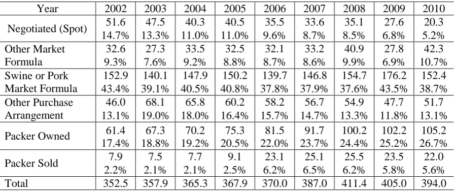
Table 1.1 reports the annual average daily hog slaughtered volumes across the six different
marketing channels. Several features are salient. First, the share of hogs transacted through the spot
(negotiated) market has steadily decreased from 14.7% in 2002 to 5.2% in 2010. It is worth
mentioning that the spot market was once the dominant marketing channel with a market share of 62%
in 1994 (Grimes and Plain, 2009). Correspondingly, the market share for AMAs has increased
steadily over the years. Among them, the most popular channels are the “Swine/Pork Market
Formula Purchases” channel, which accounted for 38.7% of hog transactions in 2010, and the “Packer
Owned” channel, which accounted for 26.7% of hog transactions in 2010. These statistics show that
though the number of hogs transacted through the spot market has decreased, the spot market still
plays a very important role in this market. This is because the transaction price for most of the
“Swine/Pork Market Formula Purchases,” is linked to the spot market price. Therefore, the spot
market remains as the place where the hog price is discovered.
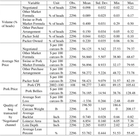
Table 1.2 presents the summary statistics for the price and quantity data by marketing channel and
2002 CPI. The number of observations for most of the variables is 2,296, which is the number of
working days between January 1st 2002 and December 31st 2010. The number of observations for
the “Packer Sold” channel is slightly less because on some days, there was no such transaction
reported. In addition to the data from MPR, we also obtained two time series of pork price data,
which will be used in our empirical analysis below. The first pork price series is the daily settlement
price of the “Pork Bellies, Frozen, 12-14 lbs” cash contracts from Chicago Mercantile Exchange
(CME). We obtained this data from the Commodity Research Bureau3 and deflated it using the 2002
CPI. The second pork price time series data we use is the monthly “Consumer Price Index—All
Urban Consumers, Pork Products” from the Bureau of Labor Statistics. We deflated the index such
that it takes the value of 100 for 2002. Both pork price time series have their own advantages and
disadvantages. The pork bellies price series has the advantage of having the same frequency as other
variables and hence providing more information. The disadvantage of this time series is the fact that
pork belly is just one particular type of pork products and therefore pork bellies price may be quite
different from the overall pork price. The advantage of the pork CPI data is that it is a better measure
for the overall price for pork products. The disadvantage of it is it is only available at the monthly
level and hence contains less information, which makes the identification of the pork price effect
more difficult.
Several other features of Table 1.2 are also worth mentioning. First, hog transactions that can be
categorized as AMAs command a slightly higher average price than hogs transacted through the spot
market. This might be due to the fact that most contracts include quality clauses which state specific
quality requirements in terms of lean percentage, loin eye depth, back fat, etc., (Vukina et al. 2007)
and the price difference simply reflects the quality premium. Second, price volatility also varies
across different marketing channels. The most volatile channels are the spot market and the “Packer
Sold” channels as prices in these channels can respond freely to the current market conditions. The
next volatile channel is the “Swine/Pork Market Formula” channel. This is not surprising as the price
for transactions in this channel are linked directly to the spot market price. The least volatile channels
are the “Other Market Formula” channel and the “Other Purchase Arrangements” channel as prices in
the former channel are linked to other commodities, which were less volatile during the sample period
and prices in the latter channel are often negotiated for a long period of time and only change once a
while. Muth et al. (2008) report similar findings. Finally, the last few rows of the table present the
summary statistics for six hog quality measures: average sort loss, average carcass weight, average
backfat, loineye area, loin depth and average lean percent.4 Except for the average backfat variable, a
higher value of the measure indicates higher quality.
1.4 Conceptual Framework
In this section, we propose a stylized model that elucidates the two channels through which AMAs
affect spot market price. As a preview, the model shows that both the number of hogs through AMAs
and spot market price volatility are key determinants of spot market price level and the effect of spot
market price volatility on spot market price is positive. Furthermore, the model also shows that spot
market price volatility is a function of the number of hogs through AMAs.
Formally, suppose there are identical farmers and identical packers in the market. There are
two marketing channels through which hogs are transacted. One is the contracts (AMAs) channel and
the other is the spot or cash market. There are also two time periods. In the first period, farmers
negotiate with packers to decide how many hogs they will supply through the contracts channel when
4 For the more detailed definition of these measures, see “7 C.F.R. PART 59—LIVESTOCK MANDATORY
the hogs are ready for slaughter in the second period. Suppose each farmer agrees to supply hogs
to packers. Therefore, a total of hogs are committed to the packers and each packer gets
hogs, where is the number of farmers per packer.5 In this period, farmers also
decide how many additional hogs to produce for the spot market in the second period. At the time
when farmers make this decision, the spot market price in the second period has not been realized yet
and hence from a farmer’s point of view, the spot market price is random. We assume the spot
market price follows a normal distribution with mean and variance .
Further assume that a farmer’s utility function exhibits the constant absolute risk aversion (CARA)
preference structure with risk aversion parameter . With these assumptions, the expected
utility for a representative farmer to produce additional hogs for the spot market can be written as
an increasing concave function of the mean-variance criterion (which corresponds to the certainty
equivalent value of revenue),
(1). ,
In (1), is the farmer’s expected revenue from selling hogs on the spot market.
represents the negative utility the farmer receives when selling on the
spot market due to the price risk. Finally, we assume the production cost function to be quadratic in
the quantity produced with parameter and hence is the increase in the
farmer’s production cost for producing additional hogs, given the fact that the farmer has already
committed to produce hogs through the AMAs channel. With these assumptions, the farmer’s
decision problem can be written as
(2).
5
and the optimal solution is,
(3).
.
The second order sufficient condition holds trivially with the assumption that both and are
positive. (3) implies that the number of hogs supplied to the spot market increases when the expected
spot market price mean increases, and decreases if the farmer is more risk averse, if the spot market
risk is higher or if more hogs are already committed through the AMAs channel.
In the second period, given the pork price in the downstream pork market and price for hogs in the
spot market, , each packer needs to decide how many hogs to procure from the spot market, in
addition to the hogs it has already obtained from the contracts channel for its processing and
packing business. We assume the market is competitive and hence each packer is a price taker. The
profit for a representative packer to procure additional hogs from the spot market and sell the pork
produced from these hogs can be written as,
(4). ,
where is the price for one pound of pork and is the number of pounds of pork that can be
produced from one hog. In (4), is the packer’s profit from procuring hogs from the
spot market and then sell the pork produced from these hogs, excluding the processing costs. The
processing cost is assumed to be quadratic in the quantity processed with parameter and hence
represents the increase in the packer’s processing cost when the packer
processes the hogs it obtains from the spot market, given the fact that it already needs to process
the hogs from the AMAs channel. In addition, in (4) represents a productivity shock for the
packer that is realized in the second period. The productivity shock is assumed to be a normally
happen with an almost zero probability. A less than 1 indicates there is a productivity gain,
possibly due to a technology improvement. A greater than 1 indicates there is a productivity loss
such as a machine breakdown.
Since in our model, the packer faces no uncertainty in the second period, no matter the packer is
risk averse or not, its decision problem can then be written as
(5).
and the optimal solution is,
(6). ,
where we have replaced with . The second order sufficient condition holds with the
assumption that is positive. (6) implies that a packer’s demand for spot market hogs decreases
with the spot market price, the number of hogs through AMAs and its processing cost, but increases
with the price of pork.
In equilibrium, the supply equals to the demand in the spot market, that is,
(8). ,
which can be rearranged to be,
(9). .
(9) yields several important implications for our study. First, (9) explains why spot market price is
random from the perspective of the farmers in the first period. This is because in the first period, pork
price and packer’s productivity shock have not been realized yet and are taken as random. Since spot
market price is a function of these two variables, it is also random. Second, the pork price, the
determinants of the spot market price level. This will guide the specification for our empirical model
below. Third, the derivative of with respect to can be derived as follows,
(10).
.
In (10), , and are positive by definition. is assumed to be positive with a probability close to
1. Also, (3) implies that must be positive. Hence, (10) implies that when spot market
price risk increases, the spot market price level will increase. When the spot market price risk
increases, it is clear from (3) and (6), that the supply to the spot market decreases and the demand for
hogs from the spot market remains the same. As a result, the equilibrium spot market price increases.
One of the main purposes of our empirical analysis below is to test this model implication. Fourth, the
derivative with respect to is,
(11). .
With the same set of assumptions discussed above, (11) implies that spot market price decreases with
the number of hogs through AMAs. This is another major hypothesis that will be tested in our
empirical analysis below. Fifth, (9) implies that
(12).
,
where is the variance for the pork price. Since we assumed above that , (12) further
implies that
(13).
.
Though not a closed form solution, (13) implies that the spot market price volatility is a function of
the number of hogs through AMAs. Our empirical analysis below will use a specification that is
Our stylized model makes it clear that there are two channels through which AMAs can affect spot
market price. The direct effect works through the effect of AMAs on demand and supply conditions
in the spot market. With more hogs committed through AMAs, (3) shows farmers supply less hogs to
the spot market. Each farmer supplies fewer hogs and hence the market supply decreases for
. Also, (6) shows that packers also demand less hogs from the spot market. Each packer
demands fewer hogs and hence market demand decreases for hogs. The reduction in demand is
larger than the reduction in supply because . Hence, (9) implies that an increase in
the number of hogs through AMAs causes a decrease in the spot market price level.
The indirect effect of AMAs on spot market price level works through its effect on spot market
price volatility. (13) implies that spot market price volatility is a function of the number of hogs
through AMAs. Total differentiating (13) with respect to and yields
(14).
(14) implies that spot market price volatility increases with the number of hogs through AMAs.
Intuitively, this is because with the increase in the number of hogs through AMAs, the spot market
becomes thinner. As a result, a given productivity shock in the second period is larger in terms of
percentages and hence the effect on spot market price is larger and the resulting price volatility is
higher. This can be seen more clearly from the derivative of with respect to using (9),
(15).
(15) implies that when the productivity shock is less favorable, decreases and the effect is larger
with a higher value of , the number of hogs transacted through AMAs. (10) further implies that
number of hogs through AMAs first increases spot market price volatility, which in turn increases
spot market price level.
1.5 Empirical Strategy and Results
1.5.1 Stationarity Test
Before we move on to regression analysis, we first need to examine whether the times series data we
have are stationary or not. As pointed out by Ng (1995), it is well known in the literature that if two
time series variables are non-stationary, then regressing one on the other will produce spurious
estimates and the standard asymptotic analysis will be invalid. If the dependent variable is stationary
and the independent variable is non-stationary, then the estimate will be consistent but the standard
asymptotic analysis will still be invalid. Therefore, if the time series data we have are found to be
non-stationary, then they need to be transformed into stationary time series data first before we can
use them for regression analysis.
One model that has been frequently used to characterize non-stationary time series data is the
so-called unit root or random walk model. As a result, testing for non-stationarity is often the same as
testing whether the time series under consideration can be characterized by a unit root or not. Many
tests have been proposed in the literature. The most widely used ones are the augmented
Dickey-Fuller test (ADF) and the Phillips-Perron test (PP). The early and pioneering work on unit root test
was done by Dickey and Fuller (1979). Specifically, they use the following AR(1) specification for a
time series variable ,
where is a white noise. The time trend variable and the intercept term need to be included in the
model when the time series shows a trend over time and a non-zero intercept. If the model has a unit
root ( ), then this series is non-stationary. So we can test the null hypothesis that against
the alternative that | |<1, which means this series is stationary. However, this specification depends
on the assumption that is a white noise. Quite often the dependence structure in is more
complicated than that of an AR(1) process and hence if the AR(1) specification of (16) is used, the
resulting error is not a white noise. To address this issue, Dickey and Fuller (1981) propose an
augmented version of their original test, now called the augmented Dickey-Fuller test, which
augments the model (16) with lags of , that is,
(17). ,
where is an appropriately chosen lag such that the resulting is a white noise series. Again, the
null hypothesis to be tested is whether or . Phillips and Perron (1988) propose
another way to address the same issue by allowing serial correlation and heteroskedasticity in the
error term and using the Newey-West (1987) procedure to correct for it. We test for the
stationarity of our time series data using both the ADF test and the PP test.
Table 1.3 reports the results of the ADF and the PP tests for the time series variables that will be
used in our regression analysis below. Whether the time trend variable or/and the intercept term are
included as controls in (16) and (17) are determined from eyeballing the time series plots of the data6
and the specification used for each variable is reported in column 2 of the Table. Column 3 of the
table reports the -statistics of the ADF test.7 For each variable, the optimal number of lags used in
(17) was chosen using the Bayesian Information Criterion (BIC) (for details, see pp. 644 of Greene
6These time series plots are at the end of the paper.
(2005)) and is reported in the parenthesis. The last column of the table reports the -statistics of the
PP test, with the number of lags used in the test taken to be the integer part of , where is
the number of time series observations. The results are almost identical across the two tests. For
most of the variables, we reject the hypothesis that there is a unit root, or the time series is
non-stationary, at the 1% significance level. For the spot market hog price series, we cannot reject the null
hypothesis at the 1% level but the MacKinnon approximate p-values for the test statistics are 0.0139
and 0.0109 in ADF and PP tests, respectively. For the pork CPI series, we fail to reject the hypothesis
that the time series is non-stationary at conventional significance levels. We, therefore, first
differenced the pork CPI series and re-tested the resulting series for unit root. Results from both tests
reject the first differenced pork CPI series is non-stationary. As a result, in our regression analysis
below, we use the first difference of the pork CPI series. For other series, we use the untransformed
series directly.
1.5.2 GARCH-M Model
To consider both the direct and the indirect effects of AMAs on the spot market price, we adopt the
generalized autoregressive conditional heteroskedasticity-in-mean (GARCH-M) model. The
GARCH-M model consists of two equations, one for spot market price level and the other for spot
market price volatility. For the price level equation, we use an autoregressive distributed lag (ARDL)
( )—autoregressive moving average (ARMA) ( ) specification as follows,
(18). ,
where denotes the spot market hog price time series, ,
, , and is the lag operator.
volatility term, (hence the name of the model, GARCH-in-mean), and pork price.
From (9), these are the main determinants of the spot market price level for hogs. In addition, we also
include in a set of monthly dummies to control for seasonality, the intercept term and the trend
variable to control for non-zero intercept and long-term trend effect in the time series data, and 5
quality measures to control for quality differences across different transaction days.8 We use the
ARDL( )-ARMA( ) specification rather than the standard ARMA( ) specification that is
often used in GARCH-M models because the former is a more parsimonious way to capture the
dependence structure of the dependent variable. Finally, is an error term that is not serially
correlated.
The second equation in the GARCH-M model models the behavior of the spot market price
volatility. We allow the possibility that the volatility varies over time and use the following
GARCH( ) specification,
(19). .
We use the specification of rather than in (19) because with this specification, the
non-negativity restriction of the GARCH model (Bollerslev, 1986) is more likely to be satisfied. As
the GARCH model is a model for the conditional variance, which, by definition, is non-negative, the
fitted value from the estimated model needs to be non-negative as well. With the specification of
in (19), the sufficient condition for the non-negativity restriction to be satisfied reduces to
be that all of the and coefficients in (19) are non-negative. Again, is a vector of control
variables including the variable of our main interest, AMAs%, as well as monthly dummies, the trend
variable and the intercept term.
8 The Loineye Area quality measure is not included in the regression analysis because it is highly correlated
We estimated many specifications of our ARDL-ARMA-GARCH model (18)-(19). Each different
combination of the lag values , , , and is a different specification. Below, we present and
discuss results from the specification that has the best fit in terms of model fitness measures AIC and
BIC.
1.5.3 Estimation Results
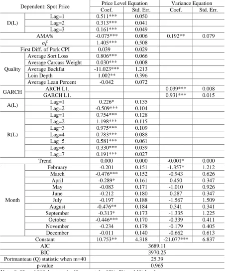
Table 1.4 presents the estimation results when the pork CPI is used as pork price. The
ARDL(3,0)-ARMA(2,7)-GARCH(1,1) specification turns out to be the specification that fits the data the best.
The results show the model is well specified. The non-negativity restriction and the stationarity
condition for the GARCH model (Bollerslev, 1986) are satisfied, since all of the ARCH and GARCH
coefficients ( s and s) in the conditional variance equation (19) are positive and the sum of them is
smaller than 1. Also, results from the Ljung-Box Portmanteau (Q) test9 show that we cannot reject
the hypothesis that the residual series from the ARDL-ARMA model (18) is not serially correlated.
This is consistent with the model assumption we made earlier. Finally, since the ARDL-ARMA
specification for the price level equation is essentially a dynamic model, there is a stability condition
that needs to be satisfied for the dependent variable to converge in equilibrium. In our context, this
means the roots of the characteristic function must be greater than one in absolute
value, where functions and are defined above in (18). Using the estimated coefficients for
s and s, we find this stability condition is satisfied as well.
9 The Q test depends on the following two facts: 1) The autocorrelation ( ) of residuals should be small; 2)
Several other results are also worth discussing. We first examine the results from the price level
equation. First, the coefficient for the AMA% variable is estimated to be negative and the estimate is
highly significant. Though not reported, we also found that this estimate was very robust across
different model specifications, always around -0.075 and highly significant. This means that the
short-run direct effect of a 1 percent increase in the share of transactions through AMAs is a reduction
in the spot market price by about 7.5 cents per 100 carcass lb (about 0.13% of the average spot market
price in the data). This result is consistent with those results from studies in the literature, which
estimate static instead of dynamic models and hence only compute the short-run effect. For example,
Elam (1992), Schroeder et al. (1993), Ward, Koontz and Schroeder (1998), Schroeter and Azzam
(2003) all reported a mild negative effect of AMAs on spot market price level in the cattle market.
This finding is also consistent with the industry arguments that AMAs decrease spot market price by
removing spot market demand while spot market supplies tend to stick to their original volumes.
Second, the coefficient for the price volatility term, or the GARCH-in-mean term, is estimated to be
positive and significant. This indicates that when there is more price risk in the market, farmers are
compensated for that. Third, pork price has a positive, though insignificant, effect on hog price level.
All these three findings are consistent with the implications of our model presented above. Fourth, all
but one quality measures have significant effects on the hog price and their signs are all correct, that
is, better quality hogs command higher price. Finally, coefficients for some of the monthly dummy
variables (March, April, August, September, October) are estimated to be negative and the estimates
are significant. This indicates that the spot market hog prices are significantly lower in those months
than in January (the reference month).
Turning to the price volatility equation, we find that as the percentage of transactions through
the arguments of market thinning effects which say that prices will more vigorously reflect a shock in
the thinner spot market resulting from the rising popularity of AMAs. This result, together with the
result that AMA% has a positive effect on price level, implies that the indirect effect of AMAs on the
price level is positive. In addition, we also find the trend variable has a negative and statistically
significant effect on price volatility. This implies that over time, the spot market becomes less
volatile. On the other hand, not much seasonality pattern is detected in the price volatility as the
estimates for all but one of the monthly dummy coefficients in the variance equation are insignificant.
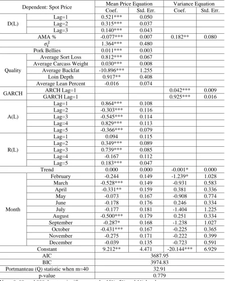
We then repeated the analysis using the other measure of pork price, that is, the daily settlement
price for cash contracts for pork bellies. Results are reported in Table 1.5. Almost all of the
coefficient estimates are similar to those of Table 1.4, both in terms of the signs and the magnitudes.
The only difference is now the pork price measure has a positive and statistically significant effect on
hog price. This is not surprising as the pork bellies price is available daily rather than monthly and
hence there is more variation in the data, which makes the identification of the coefficient easier.
1.5.4 Long-run or Equilibrium Effects of AMAs on Spot Market
Price Distribution
With the parameter estimates, we can compute the effects of AMAs on spot market price distribution.
We first examine the effect of AMAs on price volatility. Since the price volatility equation (19) is
essentially a dynamic model, the long-run or equilibrium effect of AMAs on price volatility can be
quantified using the formula
where is the coefficient for the AMA% variable in the price volatility equation. It is clear
that the effect of AMAs on price volatility varies across observations. Therefore, in Table 1.7 we
report the minimum, median, mean and maximum of this effect. When pork CPI is used as the
measure for pork price, the results indicate that one percent increase in the use of AMAs increase
price volatility by 0.0185 on average. This amounts to about 6.19% of the mean value of the fitted
price volatility, that is, , in the dataset. We also note this effect varies across observations quite a
bit, ranging from less than 1% to over 30%. The results from the case where pork bellies price is
used as the measure for pork price are quite similar.
We now turn to the effects of AMAs on spot market price level. With the ARDL-ARMA
specification (18), the long-run direct effect of AMAs on spot market price level can be computed as
(21).
,
where is the coefficient for the AMA% variable in (18). The long-run indirect effect of
AMAs on spot market price level is the product of the effect of price volatility on price level and the
effect of AMAs on price volatility, that is,
(22). = ,
where is the coefficient for the price volatility term in (18). Again, the indirect effect varies
across observations and we report its minimum, median, mean and maximum. Tables 8 and 9 report
the direct effect, the indirect effect and the net effect of AMAs on spot market price level. For the
case where pork CPI is used as pork price, on average, the direct effect of one percent increase in
AMAs decreases the spot market price by about 5 cents, and the indirect effect increases the spot
market price for about 1.75 cents. Therefore, the net effect is a reduction of about 3.3 cents per 100
period. Results from the case where pork bellies price is used as pork price show smaller effects. On
average, one percent increase in the use of AMAs leads to a 3.7% reduction in the spot market price
level. These long-run or equilibrium effects are significantly larger than the short-run effects and are
non-trivial. This is driven by the fact that the spot market hog price time series data is highly
autocorrelated and hence a small short-run effect can accumulate over time into a large long-run
effect.
Since the increase in the use of AMAs increases spot market volatility and decreases spot market
price level, we conclude that farmers who use the spot market lose because of this structural change.
On the other hand, packers gain as they pay a lower price for hogs obtained from the spot market.
1.6 Conclusions
In this paper, we estimate the effects of AMAs on spot market price distribution in the U.S. hog
market. We find increases in the use of AMAs increase spot market price volatility and decrease spot
market price level. The effect on price level is further decomposed into a direct effect, which works
through the effect of AMAs on demand and supply conditions in the spot market and an indirect
effect, which works through the effect of AMAs on spot market price volatility. The direct effect is
found to dominate the indirect effect. Increases in the use of AMAs benefit the packers and those
farmers who rely on the spot market lose.
Having obtained the results that increases in the use of AMAs have a negative direct effect on spot
market price level and this direct effect is larger than the indirect effect, the next natural question to
ask is what the main underlying driving force for this negative direct effect is. In our model, the
direct effect comes from the fact that increases in the number of hogs transacted through AMAs
represents a structural change that favors the packers. On the other hand, this effect can also come
from the fact that AMAs divert hogs of good quality away from the spot market, as studied in Wang
and Jaenicke (2006). If this is the case, then the decrease in spot market price level is less worrisome
as it simply reflects the fact lower quality hogs receive lower prices. Most likely, both effects are at
work. It is an interesting and challenging task to distinguish the two sources of the direct effect and
References
Antonovitz, F. and R. Green (1990): “Alternative Estimates of Fed Beef Supply Response to Risk,”
American Journal of Agricultural Economics, 72, 475-487.
Aradhyula, S.V. and M.T. Holt (1989): “Risk Behavior and Rational Expectations in the U.S. Broiler
Market,” American Journal of Agricultural Economics, 71, 892-902.
Bollerslev, T. (1986): “Generalized Autoregressive Conditional Heteroscedasticity,” Journal of
Econometrics, 31, 307–327.
Brorsen, B. W., J.-P. Chavas, W. R. Grant and L. D. Schnake (1985): “Marketing Margins and Price
Uncertainty: The Case of the U.S. Wheat Market,” American Journal of Agricultural Economics, 67,
3, 521-528.
Dickey, D.A. and W.A. Fuller (1979): “Distribution of the Estimator for Autoregressive Time Series
with a Unit Root,” Journal of the American Statistical Association, 74, 427-31.
Dickey, D.A. and W.A. Fuller (1981): “Likelihood Ratio Statistics for Autoregressive Time Series
with a Unit Root,” Econometrica, 49, 1057-72.
Elam, E. (1992): “Cash Forward Contracting vs. Hedging of Fed Cattle, and the Impact of Cash
Franken, J. R.V., J. M.E. Pennings and P. Garcia (2009): “Do Transaction Costs and Risk Preferences
Influence Marketing Arrangements in the Illinois Hog Industry?” Journal of Agricultural and
Resource Economics,34, 2, 297-315.
Greene, W. H. (2005): Econometric Analysis, 5th edition. Prentice Hall: Upper Saddle River, NJ.
Grimes, G. and R. Plain (2009): “U.S. Hog Marketing Contract Study,” University of Missouri
Working Paper.
Hayenga, M. L., and D. O’Brien (1992): “Packer Competition, Forward Contracting Price Impacts,
and the Relevant Market for Fed Cattle,” In Pricing and Coordination in Consolidated Livestock
Markets: Captive Supplies, Market Power, and IRS Hedging Policy, ed., W. D. Purcell, pp. 45-65.
Blacksburg VA: Research Institute on Livestock Pricing, Virginia Tech University.
Holt, M. T. (1993): “Risk Response in the Beef Marketing Channel: A Multivariate Generalized
ARCH-M Approach,” American Journal of Agricultural Economics, 75, 559–71.
Hubbard, R. G. and R. J. Weiner (1992): “Long-Term Contracting and Multiple-Price Systems,”
Journal of Business, 65, 177–198.
Just, R. E. (1974): “An Investigation of the Importance of Risk Variables in Farmers’ Production
Kavussanos, M. G., I. S. Visvikis and R. A. Batchelor (2004): “Over-the-Counter Forward Contracts
and Spot Price Volatility in Shipping,” Transportation Research Part E, 40, 273–296.
Key, N. and W. McBride (2003): “Production Contracts and Productivity in the U.S. Hog Sector,”
American Journal of Agricultural Economics, 85, 1, 121–33.
Mohapatra, S., R. E. Goodhue, C. A. Carter and J. A. Chalfant (2010): “Effects of Forward Sales on
Spot Markets: Pre-Commitment Sales and Prices for Fresh Strawberries,” American Journal of
Agricultural Economics, 92, 1, 152–163.
Muth, M. K., Y. Liu, R. Stephen and J. D. Lawrence (2008): “Differences in Prices and Price Risk
across Alternative Marketing Arrangements used in Fed Cattle Industry,” Journal of Agricultural and
Resource Economics, 33, 1, 118-135.
Newey, W. K. and K. D. West (1987): “A Simple, Positive Semi-definite, Heteroskedasticity and
Autocorrelation Consistent Covariance Matrix,” Econometrica, 55, 703-708.
Ng, S. (1995): “Testing for Homogeneity in Demand Systems When the Regressors Are
Nonstationary,” Journal of Applied Econometrics, 10, 147-163.
Phillips, P.C.B. and P. Perron (1988): “Testing for Unit Roots in Time Series Regression,”
Schroeder, T., R. Jones, J. Mintert and A. Barkley (1993): “The Impact of Forward Contracting on
Fed Cattle Transaction Prices,” Review of Agricultural Economics, 15, 325–337.
Schroeter, J. R. and A. Azzam (1991): “Marketing Margins, Market Power, and Price Uncertainty”,
American Journal of Agricultural Economics, 73, 4, 990-999.
Schroeter, J. R. and A. Azzam (2003): “Captive Supplies and the Spot Market Prices of Fed Cattle:
The Plant-Level Relationship,” Agribusiness: An International Journal, 19, 4, 489-504.
Taylor, J. L., M. K. Muth and S. Koontz (2007): “Background on Proposed Livestock Marketing
Arrangements Legislation,” Livestock & Meat Marketing Arrangements, LM-1, RTI International,
Research Triangle Park, NC.
U.S. Department of Agriculture, Agricultural Marketing Service (USDA-AMS) (1996):
Concentration in Agriculture: A Report of the Advisory Committee on Agricultural Concentration.
Vukina, T., M. K. Muth, N. E. Piggott, C. Shin, M. K. Wohlgenant, X. Zheng, S. C. Cates, M. C.
Coglaiti, S. A. Karns, J. Lawrence, J. L. Taylor and C. L. Viator (2007): “GIPSA Livestock and Meat
Marketing Study, Volume 4. Hog and Pork Industries,” Report Prepared for USDA, Grain Inspection,
Wang, Y. and E. C. Jaenicke (2006): “Simulating the Impacts of Contract Supplies in a Spot
Market—Contract Market Equilibrium Setting,” American Journal of Agricultural Economics, 88, 4,
1062–1077.
Ward, C., S. Koontz and T. Schroeder (1998): “Impacts from Captive Supplies on Fed Cattle
Transactions,” Journal of Agricultural and Resource Economics, 23, 2, 494–514.
Ward, C., S. Koontz, T. Dowty, J. Trapp and D. Peel, (1999): “Marketing Agreement Impacts in an
Experimental Market for Fed Cattle,” American Journal of Agricultural Economics, 81, 2, 347-358.
Wohlgenant, M. K. (2010): “Modeling the Effects of Restricting Packer-Owned Livestock in the U.S.
Swine Industry,” American Journal of Agricultural Economics, 52, 3, 369-375.
Zheng, X., T. Vukina and C. Shin (2008): “The Role of Farmers’ Risk Aversion for Contract Choice
Table 1.1: Average Daily Transaction Volume (# of Heads in Thousands)
Year 2002 2003 2004 2005 2006 2007 2008 2009 2010
Negotiated (Spot) 51.6 47.5 40.3 40.5 35.5 33.6 35.1 27.6 20.3 14.7% 13.3% 11.0% 11.0% 9.6% 8.7% 8.5% 6.8% 5.2% Other Market
Formula
32.6 27.3 33.5 32.5 32.1 33.2 40.9 27.8 42.3
9.3% 7.6% 9.2% 8.8% 8.7% 8.6% 9.9% 6.9% 10.7%
Swine or Pork Market Formula
152.9 140.1 147.9 150.2 139.7 146.8 154.7 176.2 152.4 43.4% 39.1% 40.5% 40.8% 37.8% 37.9% 37.6% 43.5% 38.7% Other Purchase
Arrangement
46.0 68.1 65.8 60.2 58.2 56.7 54.9 47.7 51.7
13.1% 19.0% 18.0% 16.4% 15.7% 14.7% 13.3% 11.8% 13.1%
Packer Owned 61.4 67.3 70.2 75.3 81.5 91.7 100.2 102.2 105.2
17.4% 18.8% 19.2% 20.5% 22.0% 23.7% 24.4% 25.2% 26.7%
Packer Sold 7.9 7.5 7.7 9.1 23.1 25.1 25.5 23.5 22.0
2.2% 2.1% 2.1% 2.5% 6.2% 6.5% 6.2% 5.8% 5.6%
Table 1.2: Summary Statistics for the Finished Hog Purchase Data
Variable Unit Obs. Mean Std. Dev. Min Max
Volume (% of heads)
Negotiated % of heads 2296 0.098 0.032 0.02 0.22
Other Market
Formula % of heads 2296 0.089 0.025 0.03 0.17
Swine or Pork
Market Formula % of heads 2296 0.400 0.031 0.29 0.50
Other Purchase
Arrangement % of heads 2296 0.150 0.034 0.05 0.32
Packer Sold % of heads 2296 0.044 0.021 0.00 0.10
Packer Owned % of heads 2296 0.220 0.035 0.06 0.36
Average Net Price
Negotiated
$ per 100
carcass lb 2296 56.125 9.342 27.53 79.37 Other Market
Formula
$ per 100
carcass lb 2296 56.860 5.507 38.80 68.67 Swine or Pork
Market Formula
$ per 100
carcass lb 2296 56.896 8.933 32.17 79.95 Other Purchase
Arrangement
$ per 100
carcass lb 2296 58.272 5.226 48.72 73.78
Packer Sold
$ per 100
carcass lb 2294 58.421 9.079 31.57 82.19
Pork Price
Pork CPI 2002=100 108 98.277 3.401 89.15 105.61
Pork Bellies $ per 100
carcass lb 2296 76.185 14.94 38.76 128.48
Quality of hog transacted by ‘Negotiated’ channel Average Sort Loss
$ per 100
carcass lb 2296 -1.336 0.266 -2.68 -0.69 Average
Carcass Weight lb 2296
196.50
6 3.345
186.6
0 208.17
Average
Backfat Inch 2296 0.740 0.028 0.66 0.82
Loineye Area Inch 2296 6.854 0.160 6.05 7.36
Loin Depth Inch 2296 2.285 0.053 2.02 2.45
Average Lean
Table 1.3: Unit Root Test Results
Variables Controls Augmented
Dickey-Fuller Test
Phillips–Perron Test
Spot Market Price a (Intercept) -3.32(12)** -3.40**
AMA (%) a and t (Trend) -6.77(14)*** -35.96***
Pork Price
Pork CPI a -2.46(1) -2.43
First Diff. of Pork CPI - -5.61(1) *** -7.77***
Pork Bellies a -4.10(1)*** -4.23***
Quality (Spot Market Channel)
Average Sort Loss a and t -3.94(9)*** -17.86***
Average Carcass Weight a and t -4.26(11)*** -15.77***
Average Backfat a and t -4.40(9)*** -28.25***
Loin Depth a and t -5.28(9)*** -22.89***
Average Lean Percent a and t -3.60(9)** -23.35***
Table 1.4: GARCH-M Estimation Results: Using Pork CPI as Pork Price
Dependent: Spot Price Price Level Equation Variance Equation
Coef. Std. Err. Coef. Std. Err.
D(L)
Lag=1 0.511*** 0.050
Lag=2 0.313*** 0.041
Lag=3 0.161*** 0.049
AMA% -0.075*** 0.006 0.192** 0.079
1.405*** 0.508
First Diff. of Pork CPI 0.039 0.029
Quality
Average Sort Loss 0.806*** 0.066
Average Carcass Weight 0.030*** 0.008
Average Backfat -11.023*** 1.213
Loin Depth 1.002** 0.396
Average Lean Percent -0.042 0.072
GARCH ARCH L1. 0.039*** 0.008
GARCH L1. 0.931*** 0.015
A(L) Lag=1 0.226* 0.135
Lag=2 -0.509*** 0.104
R(L)
Lag=1 0.754*** 0.128
Lag=2 1.198*** 0.115
Lag=3 0.975*** 0.109
Lag=4 0.783*** 0.088
Lag=5 0.581*** 0.061
Lag=6 0.330*** 0.039
Lag=7 0.191*** 0.027
Trend 0.000 0.000 -0.001* 0.000
Month
February -0.201 0.151 -1.357* 1.212
March -0.476*** 0.152 -0.943 0.626
April -0.289* 0.161 0.450 0.347
May -0.083 0.171 -1.010 0.926
June -0.212 0.180 0.287 0.347
July -0.197 0.188 -1.567 1.509
August -0.476** 0.184 0.341 0.341
September -0.313* 0.173 -1.335 1.225
October -0.446*** 0.170 -0.339 0.411
November -0.234 0.178 -0.179 0.405
December -0.011 0.140 -0.662 0.613
Constant 10.753** 4.318 -21.077*** 6.837
AIC 3689.11
BIC 3970.25
Portmanteau (Q) statistic when m=40 25.39
p-value 0.965