MOLECULAR EVOLUTION AND POLYMORPHISM IN A RANDOM ENVIRONMENT

(1)

JOHN H. GILLESPIE

Department of Biology. Uniuersity of Pennsylvania, Philadelphia, Pennsylvania 19104

Manuscript received June 8, 1978 Revised copy received February 20,1979

ABSTRACT

A model of multi-allelic selection in a random environment, the SAS-CFF model, is examined for compatability with allele frequency and genetic distance data acquired by electrophoresis. The symmetric version of the model tends to predict higher than observed levels of polymorphism unless substantial positive autocorrelations in the environment are postulated. The actual allele frequency configurations observed in nature are in rough agreement with those predicted by the SAS-CFF model. An approximate analysis of the transient properties of the SAS-CFF model shows that, in broad outline, the behavior is quite similar to that of the neutral model.

O N E of the major accomplishments of the neutral allele theory has been to provide a model that can simultaneously account for enzyme polymorphism and molecular evolution. In fact, under this model, enzyme polymorphism is viewed as a “phase of molecular evolution” (KIMURA and OHTA 1971). To date, models of natural selection have not achieved this broad level of applicability. Most work has focused on genetic polymorphism and has ignored the question of molecular evolution. This contributes, no doubt, to the increasing frequency with which evolutionary patterns are explained in the context of the neutral allele theory.

The major technical obstacle to developing theories of evolution and polymorphism in selectionist models is the high dimensionality of the state space. Both asymptotic and transient states of multidimensional diffusions are difficult to describe. In the neutral model, this is not a serious problem since the frequency of any particular allele is a Markovian variable whose properties can give quite a bit of information about the entire process. I n selectionist models, individual allele frequencies are not Markovian variables, making the techniques used to investigate the neutral model inapplicable. There are, however, certain ways of examining selectionist models that provide insight into their evolutionary dynamics. These ways will be exploited i n this paper to describe the dynamics of the so-called SAS-CW model of selection in a random environment (GILLESPIE 1978).

The SAS-CFF model was developed to account simultaneously for observations on the quantitative genetics of fitness traits and on enzyme polymorphisms. The model incorporates a stochastic additive scale (SAS), which is a stochastic process

(2)

reflecting spatial and temporal fluctuations in the environment, as well as the additive nature of enzyme activity in heterozygotes; and a concave fitness function (CFF)

,

which maps the stochastic additive scale to fitness. More formally, we could describe the one-locus model by a series of postulates:

( 1 ) Each homozygous genotype is characterized by a random variable,

Yi ( n , T )

,

which will be called the enzyme activity of the genotype. The enzyme activity will generally fluctuate at random in both time and space, the arguments referring to the nth patch in the Tth generation. The

i

refers to the ith allele.

( 2 ) The enzyme activity of a heterozygote is exactly intermediate between the activities of the two associated homozygotes. If we refer to the activity of the A , A , homozygote as Y i ( n , T ) , then the activity of the A , A j heterozygote will be

( 3 ) There exists a function, (~(y), which maps the activity of the enzyme onto the fitness of the genotype.

It

is assumed that this fitness function is strictly monotonically increasing, is concave throughout its domain, and approaches a finite limit as y + w . That is, +'(y)>O,+"(y)<O, and + ( y ) < K < w . The compatability of this model with experiments on the quantitative genetics of fitness traits is covered in GILLESPIE (1978).

The dynamic properties of the SAS-CFF model, like those of the neutral model, can be approximated by a multidimensional diffusion process with a single parameter, B. I n order to achieve this approximating diffusion model, various assumptions about the moments of the Yi(n,T) and about the structure of the

environment must be made. In this paper, we will deal only with the symmetric SAS-CFF model, so that we will assume that

[Yi(n,T)

+

Yj(n,T')]/2.

Thus, all homozygotes have the same mean and variance of their enzyme activities. The parameter T is introduced as a scaling factor that will be allowed to approach zero in order to arrive at the limiting diffusion model. The form of the diffusion is insensitive to the assumptions made about the structure of the environment. The state space of this process is the vector X ( t ) = [ X , ( t ) , X 2 ( t ) ,

.

, X K

( t )

1,

where

Xi

( t ) represents the frequency of the ith allele. Since there

are K segregating alleles,

K

z

X , ( t ) = l

.

j=1

(3)

MOLECULAR EVOLUTION A N D POLYMORPHISM 739 is the homozygosity of the population (GILLESPIE 1977). The asymptotic density of this process is the Dirichlet distribution

r(2B-2) IC (2B-2)/K-l

rI xi

r

( (2B-2) / K ) i=i

The expected homozygosity at equilibrium is given by

1 1 2B-2

2B--1

K

2B-1 EF=-f--.

As K+ m, that is, as we go from a finite to a n infinite-allele model, the

distribution approaches the Poisson-Dirichlet limit, and the expected gosity approaches

1

E F = - .

2B- 1

( 5 )

( 6 )

Dirichlet homozy-

(7) Thus, the asymptotic densities of the finite and infinite allele versions of the SAS-CFF model are of the same form as the symmetric neutral allele model densities.

This paper will explore three aspects of the SAS-CFF model. First, data on enzyme variation will be used to place bounds on the probable numerical value of B. Second, the initial rate of change of the genetic distance between two isolated populations will be examined in order to compare the evolutionary rate of the SAS-CFF model with that of the neutral model. Third, the transient distribution of the genetic identity of two isolated populations will be examined. The general conclusions are that evolutionary dynamics of the SAS-CFF model are similar to those of the neutral model and could not be distinguished from the neutral model at the level of resolution of the currently available data on molecular evolution or on the distribution of genetic distances between taxa.

In the symmetric SAS-CFF model, the parameter B plays a role analogous to 8 in the neutral model.

In

fact, when 2(B-1) equals 8, the asymptotic densities of both models are identical. The unfortunate aspect of the parameter B is that it does not represent a simple biological quantity as 8=4Nu does. In general, the values of B will depend on the amount of dominance, on the amount of temporal autocorrelation in the environment, and on the amount and kind of environmental subdivision of the environment. (For the details of this dependence, see GILLESPIE 1978). These details need not concern us, however, when using certain kinds of data to estimate the numerical value of B.

(4)

a0

-

alleles

-

exact

10

-

alleles

-

approx.

0

0.029 0.113

(B

-1)

I

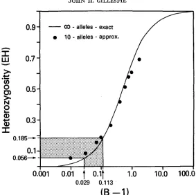
FIGURE 1.-The relationship between B-1 and heterozygosity. The dots represent the relationship f o r the approximate process ( 3 5 ) with K = 10 alleles.

corresponds to B values of 1.029 to 1.113 (Figure 1). To arrive at this use, (7) to derive the expected heterozygosity

EH is the function plotted in Figure 1.

How can this range of B values be reconciled with the underlying biology of the SAS-CFF model? T o explore this question, we will first examine the B value for an infinite-allele model where there are nonautocorrelated temporal fluctuations in an environment with no spatial heterogeneity. I n this case

B = 2 ( 1 -+"/2+") ₍₉₎

(GILLESPIE 1978), where

+

is the fitness function with the derivatives evaluated at one. It was argued in GILLESPIE (1976) that, for the fitness function

the data on the quantitative genetics of viability suggest that .a =: 0.06. Substi- tuting this into (9), we get

(5)

MOLECULAR EVOLUTION A N D POLYMORPHISM 74 1

This would correspond to an average heterozygosity of about 0.9, which is far above the range observed in nature. In a sense, we are in the same dilemma that AYALA, POWELL and

TRACY

(1972) put the neutral-allele hypothesis into by suggesting that there were fewer alleles segregating in natural populations than the theory predicts. In our case, however, there are other models of environmental fluctuations that can lower the B value to give better agreement with the

B value estimated from enzyme heterozygosities. Among these possibilities are asymmetries in the enzyme activities or nonequilibrium. These possibilities will be investigated in another paper. Here we will consider only possibilities that are possible within the context of the symmetric, equilibrium SAS-CFF model. For symmetric SAS-CFP models, environmental subdivision has the effect of raising the B values, so that the addition of a patchy structure can only make matters worse. On the other hand, positive autocorrelations in the environment have the effect of lowering the B value. For a single patch in a weakly autocorrelated environment (terminology of GILLESPIE and GUESS 1978), the B value is given by

B = ~ ( ~ - ~ / c Y ) / ( ~ - c z )

,

(12) where a is a measure of the strength of the autocorrelation. The values of a range between zero for a completely autocorrelated environment (i.e., nonfluctuating) through one for independent environments. Values larger than one correspond to negatively autocorrelated environments. Given a 0.06, we require a =: 0.067

in order to have a B value of 1.1

,

which is typical of the enzyme polymorphism data. This indicates that one viable explanation for the low heterozygosity observed in nature would be that the environmental fluctuations are positively autocorrelated. Of course, if further work on hidden alleles reveals generally higher heterozygosities, then we would lower the a value appropriately.

If

the data are so extreme as to yield B values in excess of

35,

then we could invoke environmental subdivision to raise the value. Finally, if we incorporate restricted migration, this could also result in either higher or lower heterozygosities, depending on the structure of the fluctuations. Until the data on polymorphism are more complete, a final decision on the nature of the environmental fluctuations must be postponed. However, it is clear from the above that the SAS-CFF models can, in principle, make use of two sorts of data-those on the quantitative genetics of viability and on enzyme polymorphism-to make critical inferences on the process of selection in natural populations.

In the foregoing, we used enzyme data to estimate B, but this, in itself, does not provide a test of the agreement of the data with the Poisson-Dirichlet density of the infinite-allele SAS-CFF model. However, since the neutral-allele model also has an asymptotic Poisson-Dirichlet limit, the recent work of FUERST, CHAKRABORTY and NEI (1977), which argues for the agreement of enzyme data with the neutral-allele model, may also be used to argue for agreement of these data with the SAS-CFF model. In particular, the mean and variance of heterozygosity for the SAS-CFF model:

2B-2 4 ( B - I )

2B- 1 (2B-1) '2B (2B+1)

(6)

show the same functional relationship to each other as they do in the neutral- allele model. It is this relationship that

FUERST,

CHAKRABORTY and NEI (1977) exploited in their test of the agreement of data with the Poisson-Dirichlet distribution of allele frequencies. Thus, two claims about the variable-environment selection model by FUERST, CHAKRABORTY and NEI (1977) are clearly incorrect:

(1) “In this hypothesis, the agreement of the observed variance and the expected

( 2 ) “According to this hypthesis, the heterozygosity for a given locus should not variance of the mutation-drift hypothesis must be accidental.”

vary extensively among related species.”

These two statements appear on page 475 of

FUERST,

CHAKRABORTY and

NEI

(1977).

NEI, CHAKRABORTY and FUERST (1976) made an intriguing modification of the neutral-allele model that allows for locus-by-locus variation in the mutation rate. In particular, they assumed that the mutation rate was gamma-distributed and estimated the mean and variance in the rate using data on the rates of evolution of proteins. I n a similar way, we could allow locus-by-locus variation in B values, although at the present time we are unable to find a n independent method of esti- mating the distribution of B . This variation in B would reflect the very plausible notion that certain loci experience types of environmental fluctuation different from that of other loci. If B were gamma-distributed, then the agreement of data with the variable-mutation rate neutral model would argue equally for a variable-B SAS-CFF model. This point will be taken up again when the distribution of genetic distances is examined in the next section.

As a final point, it is often argued that there should be a simple relationship between the variance in the environment and the level of heterozygosity in variable environment models. For example, OHTA (1976) uses the fact that “attempts to find correlations between heterozygosity and ecological conditions have not been successful’’ to argue against the relevance of “positive Darwinian selection” to the evolution of enzymes. More recently, POWELL and WISTRAND (1978) claimed that “there should be a positive correlation between the heterogeneity of environments and the amount of genetic variation of populations living in them.” However, the value of B, and consequently the average heterozygosity, are independent of the variance U*. Thus, in the symmetric SAS-CFF model, we would not expect a relationship between U* and H . This somewhat surprising observation

stems from the fact that the variance enters both the drift coefficient and the diffusion coefficient of the diffusion model as a constant multiple. Increasing the variance increases both the centripetal and centrifugal aspects of the process in direct proportion, so that the two influences exactly cancel. This property does not hold, however, for asymmetric models.

GENETIC IDENTITY

(7)

MOLECULAR E V O L U T I O N A N D P O L Y M O R P H I S M 743

shown that the major features of the data are in essential agreement with the statistical properties of the neutral-allele model. It would be interesting to see if the dynamic properties of the genetic distance between two isolated

SAS-CFF

populations behaved in a similar fashion. Unfortunately, the transient solution to the diffusion (3) is not available, so that we must resort to an approximate treatment of the dynamic behavior of genetic distance. Before undertaking this approximate treatment, we will first make an effort to set a time scale for change under the SAS-CFF model.

We begin by establishing the definition of genetic identity that will be utilized. In this, we follow

NEI

(1972) exactly. Consider a pair of populations with the ith allele in one of the populations being

Xi

and the frequency of the same allele in the other population being Yi. For this locus, the primitive statistics are the random variables

j z and

j y are the homozygosities of the two populations, while jzzr is the probability of identity of two alleles, one chosen at random from each of the two populations. These random variables were used by

NEI (1972)

to define two different measures of genetic identity. In the first instance, we have the normalized genetic identity of the jth locus, which is the random variable

In the second instance, we have what NEI ( 1972) called the normalized identity of genes with respect to all loci, which is the ratio of expectations

Of course,

E I j Z I

.

To set the time scale of the change of genetic distance under the SAS-CFF model, we will examine the instantaneous rate of change of I at the first moment of isolation of two populations that are derived from a single equilibrium population. Since the process starts at equilibrium, we have

I

We cannot calculate Ejxy, but we can calculate

(8)

744

I n this calculation, we use the fact that the second-order derivatives with respect to xi or yi are zero. We now take the expectation of ( 2 0 ) with respect to ( 5 ) and let K+ 00

,

giving

-2(B-1) - -2 (B-I )

- * EF

’

= (2B-1) ( 2 B f l ) 2 B f l To obtain the rate of change of I , we divide by EF giving

- 2 ( B - I )

2Bfl

This rate, which lies between zero and one, is analagous to the rate -0 = -4Na, which is obtained from the normalized neutral model. In the neutral model, time is measured in units of 2N generations, so that the rate in “real time” is given by

-e

2 N -

Y ( 2 3 )

as given by NEI (1972). In deriving the diffusion equations for the SAS-CFF model, the time scale was also normalized. For a model with a single patch plus autocorrelations, the normalization was written as

(GILLESPIE 1978), were T is a variable that is introduced for technical reasons. If we suppress T and let u2 be the actual variance rather than U ~ T being the actual variance, we can write the “real time” rate as

-2 (B-I )

_.

u2 (1-p)

4 ’ 2 (2/a- 1 )

2 .

2Bfl

v =

I n this expression we know, approximately, that B =: 1.1, +’2 =: 0.0032 and

a =: 0.067, giving

IvI 0.0014u2(1-p)

.

(2.6)

W e are left with an expression for the rate of change of I at the moment of isolation that depends on the parameters u2 (1 -p)

.

If we knew the average rate of change of genetic identity at the moment of isolation, we could estimate these parameters. Since this information is not available, we can at least ask the follow- ing question: What value would m2 ( l - p ) have to have in order for the rate of change of genetic identity under the SAS-CFF model to equal the rate of change under the neutral model? The neutral rate of change is obtained from gene sub- stitution data and is generally estimated on a per cistron level to be I v / = lo-’ to

IO+. For the desired agreement, we require

(9)

MOLECULAR EVOLUTION A N D POLYMORPHISM 745

If

p = 0, this would correspond to a standard deviation of enzyme activity of roughly 0.01 to 0.032. These calculations are necessarily crude, but indicate that the SAS-CFF model, with the same asymptotic density as the neutral model, initially evolves at about the same rate as the neutral model if U' ( 1 -p) = 1

e4

to Thus, the SAS-CFF model can share the property of polymorphism, plus slow evolutionary change, which was thought to be uniquely characteristic of the neutral model.

We now turn to the distribution of Zj between two isolated populations that are drawn from an equilibrium SAS-CFF population. We will use an approximate analysis that has tremendous potential in the present context, as well, as for other problems associated with transient states of the SAS-CFF model. The basic idea is to find a process similar to ( 3 ) , but whose complete transient solution can be obtained. If we write the drift coefficient of ( 3 ) in the form

Edxi = [zi(F-zi)+(B-l)zi(F-zi)]dt

,

( 2 8 ) it is tempting, given the smallness of (B-1), to seek an approximate process of the form

Edzi = [ z i ( F - ~ i )

+

( B - l ) g ( ~ ) ] d t

,

(29)

where g(z) is a convenient function. I n this way as (B-l)-tO, the original and the approximate processes approach the same process and, presumably, each other.

To arrive at a convenient approximating process whose transient densities can be explicitly determined, we first transform ( 3 ) to the new process

~i = l n ( ~ i / ~ K ) , i=l, 2,.

.

K-1

.

₍₃₀₎

Then it is easy to show that the new process has drift and diffusion coefficients

Edui = [ ( B - I ) ( l - e u i ) / ( l f ~ e u ~ ) ] d t Eduiduj = (l+Sij)dt

.

If we now linearize the drift coefficient around ui = 0, we get a new process with the same diffusion coefficient, but with the new drift coefficient

-(B-1)

K ui

.

Edui =

This process is a ( K - 1 ) -dimensional Orstein-Uhlenbeck process of a particularly simple form. Its transient densities are Gaussian with mean

-(B-l)

- t

E u i ( t ) = ui(O>e

and second order moments

-2(B-1)

t

[I-e ]

K B-I

VAR u i ( t ) =-

-2 IB-1)

(33)

( 34)

, , t

[I-e

1 .

K 2(B-1)

(10)

This process can now be transformed back to the allele frequency process. When this is accomplished, we get the approximating process

1 "

Edzi { z i ( F - z i )

+

( B - 1 ) - [

X

Z j

lnzj

-

l n z i ] } d t

K

~ = 1

(35)

EdZidzj

= z i ~ j ( S i j

4-

F - ~ i z j ) d t -

.

This approximating process has the same diffusion coefficients as the original process, but differs in the form of the drift coefficient. For B 1, we expect

this

process to behave very much like the SAS-CFF process.

Since we know the solution to the process ui, we can easily obtain the transient solution to hte process zi. Let

where

2 ( B - I )

K

A =

-A

t m i ( t ) = In[zi(O)/q(O)]e2

.

W e can now write the transient density of (35) as

where

yt =

dK

[27r~-1( I -e-it ) ] (K--1)/2

The asymptotic density of (35) is given by (38) with

(37)

(38)

(39)

(11)

MOLECULAR EVOLUTION A N D POLYMORPHISM

747 0 2

+I'

0.1 a,

0

.I

yl

Y-

@

o

s

E

0'

-0.1

-0.2

B=l.5 approx. B=1.5 exact

----

-

_.-._

B = l . l approx. and exact

0

0.2

0.4

0.6

0.8

1 .o

Allele

Frequency

FIGURE 2.-A comparison of the drift coefficients for the two-allele version of the exact and approximating process.

higher heterozygosities than predicted by the exact model, as well as a lower variance in heterozygosity. This is illustrated in Figures 1 and 3. For B close to one, the agreement is quite good, although it deviates in the expected direction of excessive heterozygosity. For large B, the heterozygosity is too low. This is due to the fact that there are a finite, rather than an infinite, number of alleles i n the approximating process. For B close to one, the finiteness of the number of alleles becomes irrelevant.

The value of the approximating process lies, in part, in the ease with which it can be used to generate allele-frequency configurations on a computer. This property will now be exploited to examine the distribution of Z j . The simplest

way to generate this distribution is first to generate equilibrium configurations, and then to generate two further configurations with the equilibrium configura- tion as the initial point and with the desired value of t. The random variable Z j

is then calculated for these two populations. This experiment is repeated many times and the distribution of Z j may be displayed as a histogram. In carrying out

this approach, all of the computations are routine except for the desirability of a fast normal random variate generator. In these Monte-Carlo calculations, the decomposition method given in NEWMAN and ODELL (1971) was used to generate the normal deviates.

(12)

0.08

LL

rc 0.06

0

Q1

0 c

Q

.-

3

0.04

0.02

0 0.2 0.4 0.6 0.8 1

.o

F

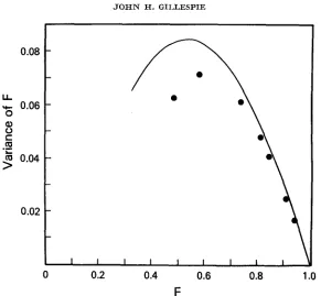
FIGURE 3.-The line is the relationship between the mean and variance of F for the Poisson- Dirichlet limit; the dots for the results of the approximating process (35).

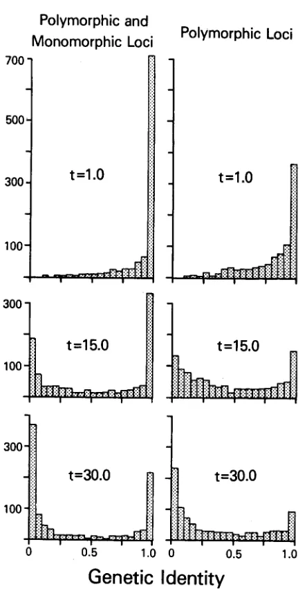
all trials, as well as those trials for “polymorphic populations” that are trials in which at least one of the two derived populations the most frequent allele has a frequency of less than 0.95. This should be compared to the analagous histograms in AYALA and GILPIN (1974) and NEI and TATANO (1975). Th’ is comparison reveals that the SAS-CFF model behaves in a manner that is very similar to the neutral model when histograms of Zj are visually compared in the cases of “monomorphic” plus “polymorphic” populations. This is not surprising, since both models are constrained to having relatively low heterozygosities and, therefore, most I f values will be near zerG or one with relatively few in the middle of the unit interval. The temporal sequence of J-shaped to U-shaped to reflected J-shaped distributions will be displayed by essentially any evolutionary model with constant rates of evolution and low heterozygosities. From this we must conclude that histograms of

Zi

may not be useful in distinguishing the neutral allele model from the SAS-CFF model, or, presumably, from any other Ftationary model of evolution with low heterozygosities.

In the case of polymorphic populations, the SAS-CFF model exhibits a bimodal shape, which AYALA (1977) showed is characteristic of the Drosophila data, but is not exhibited by the neutral-allele model. This property suggests that the SAS- CFF model may be preferable to the neutral model as an explanation f o r enzyme polymorphism in Drosophila.

(13)

MOLECULAR EVOLUTION A N D POLYMORPHISM

Polymorphic and

Monomorphic Loci Polymorphic Loci

300

100

300

100

0 0.5 1

.o

0 0.5 1

.o

749

Genetic I

dent

ity

FIGURE 4.-Histogram for genetic identities based on 200 replicates with B = 1.1.

distance data quite a bit further than the simple visual inspection of histograms. They have looked at the functional relationships between genetic distance and the correlation of heterozygosity, and between the mean and variance of genetic distance under the neutral-allele model. These relationships are compared to enzyme data. The agreement is variable, but there is no compelling reason to reject the neutral-allele theory on the bases of these comparisons except, perhaps, for Drosophila.

(14)

750

both cases, we will be interested in both the quantitative and the qualitative aspects of the comparison between these relationships for the neutral-allele and the SAS-CFF models.

Genetic identity and correlation of heterozygosity

tion between heterozygosities, r, are related by

OHTA (1976) showed that the genetic identity given by (16) and the correla-

(41)

TZ 12(1+1/8)

.

The correlation, as a function of

I,

depends only on the single paramater 8, which may be estimated independently. This should, i n principle, provide a test for the neutral-allele model. The relationship between r and

I

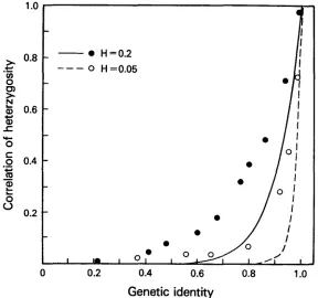
for the approximate SAS-CFF model is given in Figure 5 for the heterozygosities H = 0.05 and

H

= 0.02. The curves are the relationship (41) for the neutral model for these same heterozygosities. W e see from this figure that the drop off of the correlation of heterozygosity with genetic identity is slower under the SAS-CFF model than under the neutral model. I t is also apparent from this figure that the functional dependence of r and I depends on the heterozygosity of the population. This is contrary to the claim of CHAKRABORTY, FUERST and NEI (1978) that, under a random fluctuation model, “the correlation should occur irrespective of the level

- 0

0

---

H

= 0.2

H =0.05

0

I

J

0

I Im I 0:

,

0 0.2 0.4 0.6 0.8 1

.o

Genetic identity

(15)

MOLECULAR EVOLUTION AND POLYMORPHISM

75 1

of heterozygosity.” Comparison of Figure 4 with Figure 3 of CHAKRABORTY,

FUERST

and NEI (1978) shows that the SAS-CFF model fits the data better than does the neutral-allele model with constant mutation rate, but does not fit as well, in the case of Drosophila, as the neutral model with variable mutation rates. We can, however, modify the SAS-CFF model to include locus-by-locus variation in B, as discussed earlier. This will have the same effect as does varia- lion in the mutation rate and will make the agreement of the SAS-CFF model with the Drosophila data accept2ble.

Mean and variance of genetic distance

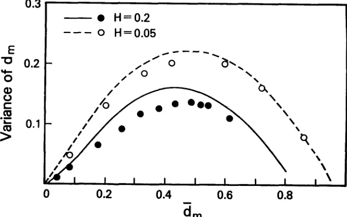
The comparison of the mean and variance of genetic distance, d,, for the neutral allele and the SAS-CFF models is given in Figure 6. For the definition of

d, and for its moments under neutrality, see CHAKRABORTY,

FUERST

and

NEI

(1 978). The form of the relationship is similar to that under neutrality although the variance under the SAS-CFF model is less than that of the neutral model for a given d*$. To some extent this will be caused by the approximation (35)

since, as demonstrated in Figure 3, the approximate process will generally show reduced variances in measures like genetic distance and heterozygosity. There is also an effect due to the fact that the Monte-Carlo program utilized only ten alleles. Nonetheless, if we accept the comparison at face value and examine Figure

5 of CHAKRABORTY,

FUERST and NEI (1978)

,

which looks at the enzyme data, we see that the SAS-CFF model will fit the data adequately for all groups except, perhaps, Drosophila, where the curve under the SAS-CFF model will

0.3 E

0

Q)

0

c

(TJ

’c1

0.2

rc

.-

5

0.1 >

H=0.2

0

H=0.05

---

\

/ e - - -

0’ 0

*,

0 0‘0

\

P

\

, \

0

0.2

0.4 _-

0.6

0.8 dml

(16)

752

fall below the data points. The curve for the constant-mutation neutral model falls above the data points, while the variable mutation neutral curve fits the data quite well.

I n summary, the behavior of genetic distance under the SAS-CFF model is qualitatively like the behavior under neutrality, although quantitatively there are differences. At the present time both behaviors seem to fit the enzyme data adequately. A definitive test will be unlikely until the problem of the non- identification

OF

alleles is resolved.

DISCUSSION

The SAS-CFF model is a model of a particular form of natural selection in a n infinitely large population experiencing no mutation. Since all natural populations are finite and all loci are mutable. it is natural to query the domain of applicability of the SAS-CFF model. The asymptotic and transient properties explored in this paper should be virtually unaffected by genetic drift and mutation if the coefficient of

xixj [ S , j

+

F

- xi - ~ j ] (42)

in the moment E A X , A X ~ is much larger than the reciprocal of the population size. For example, in the two-allele case. the combined mutation

+

drift

+

SAS-CFF model for a single patch and no autocorrelation has the drift and diffusion coefficients

(43)

E d x = { ~ B x ( 1-S) (

S-S)

+e8 (

S - X )

}

E d 2 = 22' ( 1-X) '+ex ( 1 - s )

,

where =2Na2. I t is obvious that, as E-O, the combined model approaches the simple SAS-CFF model. This is also reflected in the asymptotic density, which may be written as

c

[z ( 1

-x)

] B-2 [ 1

+

,/ex ( 1 -x)]B-1-8

.

₍₄₄₎

where [z(l-x)]B-2 will be recognized as the asymptotic density of the SAS- CFF model without the effects of drift and mutation. Thus, when 2Na2 is very large, we would not expect the infinite and the finite N models to behave very differently.

There have been other attempts to examine the evolutionary dynamics of random environment models. The two most conspicuous of these are by NEI and YOKOYAMA (1976) and by TAKAHATA, KAZUSHIGE and MATSUDA (1975). In both instances, the models included random fluctuations, genetic drift and mutation. However, in both cases the analyses make the error of assuming that the multiple-allelic aspects of selection in a fluctuating environment may be inferred from the single allelic behavior. I n particular, NEI and YOKOYAMA (1976) in- correctly assume that the diffusion coefficient for the ith allele is of the form

(17)

MOLECULAR EVOLUTION A N D POLYMORPHISM 753 where the correct form for the term reflecting the effects of a variable environment is given by (3). The entire discussion of the incompatibility of random environment models with enzyme data in NEI and YOKOYAMA (1976) must be discounted. Similarly TAKAHATA, KAZUSHIGE and MATSUDA (1 975) have assumed that one can infer multi-allelic properties from single-allele models. They have made the additional assumption that a Strotonovich-type approach io the random fluctuation equation is appropriate. For a discussion of the problems of this approach, see TURELLI (1977) or GILLESPIE and GUESS (1978).

In conclusion, this paper shows that the SAS-CFF model is in reasonable agreement with the presently available enzyme data. There is no way at present of convincingly rejecting any of a number of models that are also in reasonable agreement with the data. The main virtue of the SAS-CFF model as it is presently developed is that it addresses a wider range of phenomena than do any of the competing models.

LITERATURE CITED

AYALA, F. J., 1977

AYALA, F. J. and M. E. GILPIN, 1974

AYALA, F. J., J. R. POWELL and M. L. TRACY, 1972

Protein evolution in different species: Is it a random process? pp. 73-102. In: Malecular Evolution and Polymorphism. Edited by M. KIMARA, Mitshima, Japan.

Gene frequency comparisons between taxa: support for the natural selection of protein polymorphisms. Proc. Natl. Acad. Sci. U S . 71 : 4847-4849.

Enzyme variability in the Drosophila willis- toni group. V. genetic variation in natural populations of Drosophila equinoxialis. Genet. Res. 20: 19-42.

Statistical studies on protein polymorphism in natural populations. 11. Gene differentiation between populations. Genetic 88: 367-390.

The sampling theory of selectivity neutral alleles. Theoret. Pop. Biol. 3: 87-112.

Statistical studies on protein polymorphism in natural populations. I. Distribution of single locus heterozygosity. Genetics 86 : 455-483. A general model to account f o r enzyme variation in natural populations. 11. Characterization of the fitness function. Am. Naturalist 110: 809-821. -,

1977 Sampling theory for alleles in a random environment. Nature 226: 443-445. -,

1978 A general model to account for enzyme variation in natural populations. V. The SAS-CFF model. Theoret. Pop. Bid. 14: 1-46,

GILLESPIE, J. H. and H. A4. GUESS, 1978 The effects of environmental autocorrelations on the progress of selection in a random environment. Am. Naturalist 112: 897-909.

JOHNSON, N. L., 1949 metrika 36: 149-176. KIMURA, M. and T. OHTA, 1971

228: 467469.

LEWONTIN, R. C., 1974

NEI, M., 1972

NEI, M., R. CHAKRABORTY and P. A. FUERST, 1976

NEI, M. and Y. TATENO, 1975

CHAKRABORTY, R., P. A. FUERST and M. NEI, 1978

EWENS, W. J., 1972

FUERST, P. A., R. CHAKRABORTY and M. NEI, 1977 GILLESPIE, J. H., 1976

Systems of frequency curves generated by methods of translation. Bio-

Protein polymorphism as a phase of molecular evolution. Nature

The Genetic Basis of Evolutionary Change. Columbia Univ. Press, New York.

Genetic distance between populations. Am. Naturalist 106: 283-292.

Infinite allele model with varying mutation

Interlocus variation of genetic distance and the neutral mutation rate. Proc. Natl. Acad. Sci. US. 73: 4164-4168.

(18)

NEI, M. and S. YOKOYAMA, 1976

variability in a fi'iite population. Japan I. Genet. 51 : 355-369. NEWMAN, T. G. and P. L. ODELL, 1971

York.

OHTA, T., 1976

morphism. Theoret. Pop. Biol. 10: 254-275.

POWELL, J. R. and H. WISTRAND, 1978

petitor on genetic variation i n Drosophila. Am Naturalist 112 : 925-934.

TAKAHATA, J., I. KAZUSHIGE and H. MATSUDA, 1975

coeficient on gene frequency in a population. Proc. Natl. Acad. Sci. U.S. 72 : 4541-4545. TURELLI, M., 1977

140-178.

Effects of random fluctuations of selection intensity on genetic

The Generation of Random Variates. Hafner, New

Role of very slightly deleterious mutations in molecular evolution and poly-

The effects of heterogeneous environments and a com-

Effect of tempera1 fluctuation of selection

Random environments and stochastic calculus. Theoret. Pop. Biol. 12: