ABSTRACT
ELLISON, VICTORIA MARIE. Using Linear Programming based Exploratory Techniques in Gene Expression Consensus Clustering. (Under the direction of Yahya Fathi.)
There exist many options when it comes to clustering data including: what clustering algo-rithm to use, what preselected parameters of certain clustering algoalgo-rithms to use, and which results of certain clustering algorithms to use. Consensus clustering is useful in generating a clustering which has the most consensus with multiple differing clusterings of the same data set. However, most consensus clustering algorithms do not provide an exact optimal solution, provide the user with options as to how many clusters are in the returned consensus clustering, or reflect the nested nature of the clusters, which is a feature inherent to many data sets. These features are especially important in the analysis of gene expression profile data.
To meet the needs of these features we propose a divisive hierarchical consensus clustering algorithm, which we call CCA-β. This consensus clustering algorithm makes use of a special type of cut, which we also propose, called a β-ratio cut. We demonstrate how this β-ratio cut is a natural extension of the cluster ratio cut that incorporates finding the nested nature of a graph.
We also propose a heuristic for CCA-β, which we call CCA-ROPPPA. This heuristic applies a proposed parametric programming algorithm to a proposed parametric linear programming formulation. We create this proposed parametric linear programming formulation by modifying the BILP formulation of the Median Partition Problem (MPP) proposed by Grotschel and Wakabayashi. We create this proposed parametric programming algorithm by modifying the optimal partition parametric programming algorithm (OPPPA) proposed by Berkelaar et al.
We prove that under certain conditions a.) our CCA-ROPPPA heuristic returns a consensus clustering that is equivalent to a solution to the minimum cluster ratio problem and b.) our CCA-ROPPPA heuristic returns a set of consensus clusterings that could have been returned by our CCA-β algorithm. Using real gene expression profile data sets and artificial data sets we create sets of clusterings for which we would like to find a consensus clustering(s). We then apply CCA-ROPPPA to these sets of clusterings and assess the frequency with which these aforementioned conditions were met.
We also compare CCA-ROPPPA to two other consensus clustering algorithms. We use the same real gene expression profile data sets and artificial data sets and the same sets of clusterings created from these data sets. We then apply CCA-ROPPPA and the two other consensus clustering algorithms to these sets of clusterings and compare a.) the nature and quality of the consensus clusterings returned and b.) the execution times of the algorithms.
©Copyright 2017 by Victoria Marie Ellison
Using Linear Programming based Exploratory Techniques in Gene Expression Consensus Clustering
by
Victoria Marie Ellison
A dissertation submitted to the Graduate Faculty of North Carolina State University
in partial fulfillment of the requirements for the Degree of
Doctor of Philosophy
Operations Research
Raleigh, North Carolina
2017
APPROVED BY:
Steffen Heber Michael Kay
Amy Langville Osman Ozaltin
Yahya Fathi
BIOGRAPHY
Victoria was born and raised in Southern Maryland on the shores of the Chesapeake Bay. An early passion for problem solving combined with growing up so close to a center of change, progress, and civic engagement like Washington D.C. lead her to pursue a career path in applied mathematics where she hoped to be able to apply her problem solving skills to solving real world problems.
She completed a B.S. in Mathematics with a minor in Statistics at James Madison Univer-sity in 2008. During this time she conducted undergraduate research applying and developing statistical techniques to applications in finance and healthcare. Also during this time she applied statistical techniques to applications in transportation and population studies via her intern-ships at the Washington Metropolitan Area Transit Authority and the United States Census Bureau respectively.
Wanting to further her studies, she then completed a M.S. in Mathematics at the College of Charleston in 2010. While Victoria enjoyed statistics, she found herself desiring a career path more focused in applied deterministic modeling and having more opportunities for student outreach. It was during this time that she discovered the field of Operations Research and her passion for teaching. She found that she enjoyed the challenge of breaking down complex topics and making it readily understandable for anyone to understand. It was then she decided to purse a Ph.D. in Operations Research at North Carolina State University.
The topic for this dissertation started from research which began in her master’s program at the College of Charleston. Victoria really enjoyed the particular combination of Linear Pro-gramming and data mining techniques such as consensus clustering, so she pursued an extension of this research topic for her doctoral dissertation.
ACKNOWLEDGEMENTS
TABLE OF CONTENTS
LIST OF TABLES . . . vii
LIST OF FIGURES . . . ix
Chapter 1 INTRODUCTION . . . 1
1.1 Gene Expression Analysis . . . 1
1.2 Gene Expression Clustering . . . 3
1.3 Consensus Clustering . . . 4
1.3.1 Co-Occurence Consensus Clustering . . . 6
1.3.2 Median Partition Problem . . . 7
1.4 IP Formulation of the Median Partition Problem with Mirkin Distance . . . 8
1.5 Thesis Summary . . . 12
Chapter 2 BACKGROUND . . . 15
2.1 Graph Theory . . . 15
2.1.1 Existing Graph Theoretic Terms . . . 15
2.1.2 Proposed Graph Theoretic Terms . . . 17
2.2 Clustering and Consensus Clustering . . . 18
2.3 Divisive Hierarchical Clustering Algorithm . . . 19
2.4 Relevant Optimization Problems . . . 20
Chapter 3 PROPOSED CONSENSUS CLUSTERING ALGORITHM AND HEURISTICS . . . 22
3.1 CCA-β . . . 22
3.2 Heuristics for CCA-β . . . 23
Chapter 4 PARAMETRIC LP MODEL . . . 25
4.1 Parametric LP ModelPλ . . . 25
4.2 Related GWLP Model P . . . 27
4.2.1 GWLP ModelP . . . 27
4.2.2 How (P) Relates to (Pλ) . . . 27
4.2.3 Properties and Interpreting Solutions ofP . . . 28
4.3 Properties and Interpreting Solutions of Pλ . . . 28
Chapter 5 Parametric Programming Algorithms . . . 31
5.1 Parametric Programming Algorithm Notation and Properties . . . 32
5.1.1 Parametric Programming Algorithm Notation . . . 32
5.1.2 Parametric Programming Algorithm Properties . . . 35
5.2 Optimal Partition Parametric Programming Algorithm . . . 37
5.3 Relaxed Optimal Partition Parametric Programming Algorithm . . . 41
5.3.1 Constraint Addition Routine . . . 42
5.3.2 Algorithm . . . 43
5.4 Discussion . . . 47
Chapter 6 Structural Proofs . . . 50
6.1 Lemmas . . . 50
6.2 Theorem . . . 52
Chapter 7 Numerical Testing . . . 54
7.1 Algorithms Compared to CCA-ROPPPA . . . 56
7.2 Creating Input for CCA-UPGMA, CCA-GWLP, and CCA-ROPPPA . . . 58
7.2.1 Data Sets . . . 59
7.2.2 Create Partition Sets (Set of Input Clusterings) . . . 60
7.2.3 Create Permutation Sets and Coassociation Matrices . . . 64
7.2.4 Use Each Coassociation Matrix as Input for the Three Consensus Clus-tering Algorithms . . . 65
7.3 Computer, Software, and LP Solving . . . 66
7.4 Interpreting Consensus Clustering Results . . . 66
7.4.1 Permutation Set Names . . . 67
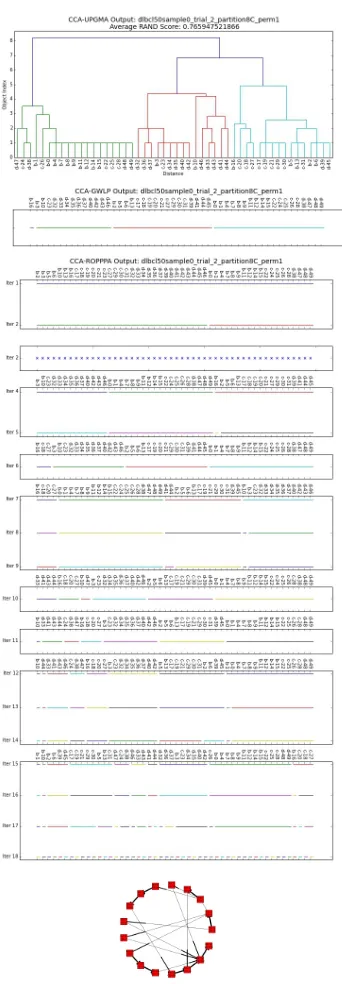
7.4.2 Interpreting CCA-UPGMA Results . . . 67
7.4.3 Interpreting CCA-GWLP Results . . . 68
7.4.4 Interpreting CCA-ROPPPA Results . . . 68
7.4.5 Examples . . . 70
7.5 Testing when CCA-ROPPPA returns a CCA-β Solution . . . 75
7.5.1 CCA-ROPPPA using Presolve in Xpress-IVE . . . 75
7.5.2 CCA-ROPPPA without using Presolve in Xpress-IVE . . . 77
7.6 Comparing CCA-ROPPPA to CCA-GWLP and CCA-UPGMA . . . 86
7.6.1 Execution Times . . . 86
7.6.2 Consensus Clustering Nature and Quality: ROPPPA and CCA-GWLP . . . 86
7.6.3 Consensus Clustering Nature and Quality: ROPPPA and CCA-UPGMA . . . 95
Chapter 8 Discussion . . . .107
8.1 Discussion of Numerical Tests . . . 107
8.1.1 Benefits and Drawbacks of CCA-ROPPPA . . . 107
8.1.2 Future Work to Address the Drawbacks . . . 108
8.2 How CCA-ROPPPA Relates to the Minimum Cluster Ratio Cut . . . 109
8.2.1 Primal and Dual Formulations Related to the UMFP . . . 109
8.2.2 Relationship between the Cluster Ratio Problem and CCA-ROPPPA . . . 115
8.3 How CCA-ROPPPA is an Extension of the Minimum Cluster Ratio Problem . . 115
8.3.1 Primal and Dual Formulations Related to an Extension of the UMFP . . 116
Chapter 9 Conclusion . . . .122
9.1 Summary of Contributions . . . 122
BIBLIOGRAPHY . . . .126
LIST OF TABLES
Table 7.1 Real and artificial data sets . . . 62 Table 7.2 CCA-ROPPPA using Presolve in Xpress-IVE: Summary Statistics Total . 77 Table 7.3 CCA-ROPPPA using Presolve in Xpress-IVE: Summary Statistics by
Orig-inal Data . . . 78 Table 7.4 CCA-ROPPPA using Presolve in Xpress-IVE: Summary Statistics by
Per-mutation Set Size . . . 79 Table 7.5 CCA-ROPPPA using Presolve in Xpress-IVE: Summary Statistics by
In-put Clustering Set Trial . . . 80 Table 7.6 CCA-ROPPPA using Presolve in Xpress-IVE: Summary Statistics by
Per-mutation Set Type . . . 81 Table 7.7 CCA-ROPPPA Using and Not Using Presolve in Xpress-IVE: Summary
Statistics . . . 82 Table 7.8 Different resulting vectors sets returned by CCA-ROPPPA when presolve
was and was not used: Summary Statistics . . . 83 Table 7.9 CCA-ROPPPA Using and Not Using Presolve in Xpress-IVE: Heuristic
Performance Summary Statistics . . . 83 Table 7.10 CCA-ROPPPA Using and Not Using Presolve in Xpress-IVE: Summary
Statistics by Data . . . 84 Table 7.11 CCA-ROPPPA Using and Not Using Presolve in Xpress-IVE: Summary
Statistics by Partition Set Size . . . 85 Table 7.12 CCA-ROPPPA Using and Not Using Presolve in Xpress-IVE: Summary
Statistics by Input Clustering Trial Set . . . 85 Table 7.13 CCA-ROPPPA Using and Not Using Presolve in Xpress-IVE: Summary
Statistics by Permutation Set Type . . . 86 Table 7.14 Summary statistics of CCA-UPGMA, CCA-GWLP, and CCA-ROPPPA
computation times on the 648 permutation sets. . . 87 Table 7.15 Percent of Permutation Sets in which CCA-GWLP Returned a Consensus
Clustering that was One of the Consensus Clusterings Returned by CCA-ROPPPA . . . 88 Table 7.16 Whether CCA-ROPPPA and CCA-GWLP Returned a Consensus
Clus-tering with the Desired or Expected Number of Clusters . . . 90 Table 7.17 Percent of Permutation Sets from this Data Set in which CCA-GWLP
Returned More than the Expected or Desired Number of Clusters . . . 92 Table 7.18 The RAND Score of the Most Desirable Consensus Clustering Returned
by CCA-ROPPPA (CCA-GWLP) and the Correct Clustering . . . 94 Table 7.19 ARS Difference Between the Permutation Sets in which CCA-GWLP Did
and Did Not Return a Consensus Clustering that was One of the Consensus Clusterings Returned by CCA-ROPPPA . . . 95 Table 7.20 The Number of Consensus Clusterings Returned by CCA-ROPPPA and
CCA-UPGMA . . . 97 Table 7.21 Percent of Permutation Sets in which the Results of CCA-UPGMA were
Table 7.22 Whether CCA-ROPPPA and CCA-UPGMA Returned a Consensus Clus-tering with the Desired or Expected Number of Clusters . . . 101 Table 7.23 The RAND Score of the Most Desirable Consensus Clustering Returned
by CCA-ROPPPA (CCA-UPGMA) and the Correct Clustering . . . 102 Table 7.24 The Differences Between the Permutation Sets in Which the Results of
CCA-UPGMA were Different than those of CCA-ROPPPA: by Original Data . . . 104 Table 7.25 The Differences Between the Permutation Sets in Which the Results of
CCA-UPGMA were Different than those of CCA-ROPPPA: by Input Clus-tering Trial . . . 105 Table 7.26 The Differences Between the Permutation Sets in Which the Results of
CCA-UPGMA were Different than those of CCA-ROPPPA: by Partition Set Size . . . 105 Table 7.27 The Differences Between the Permutation Sets in Which the Results of
LIST OF FIGURES
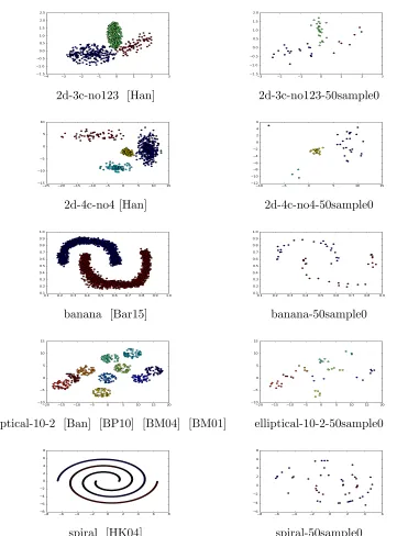
Figure 7.1 Artificial data sets and their random samples of 50 objects . . . 61
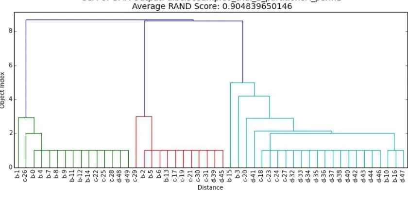
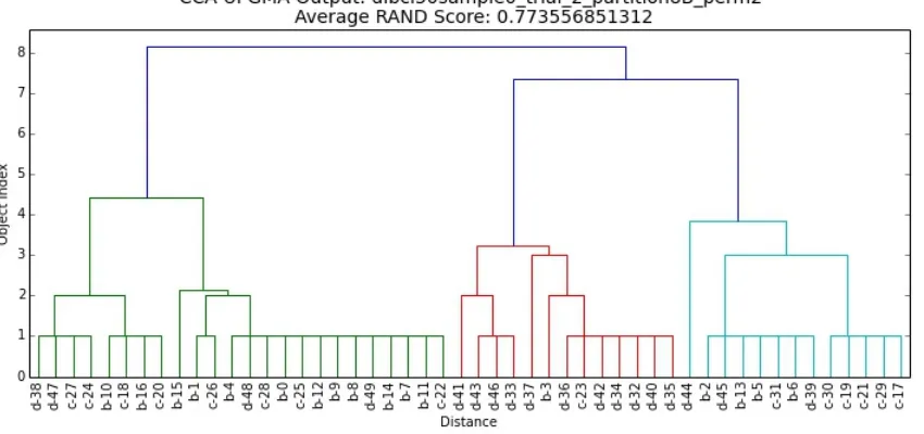
Figure 7.2 Results for dlbcl50sample0-trial-2-partition8A . . . 72
Figure 7.3 Results for dlbcl50sample0-trial-2-partition8A-perm1 . . . 73
Figure 7.4 Results for dlbcl50sample0-trial-2-partition8-perm2 . . . 74
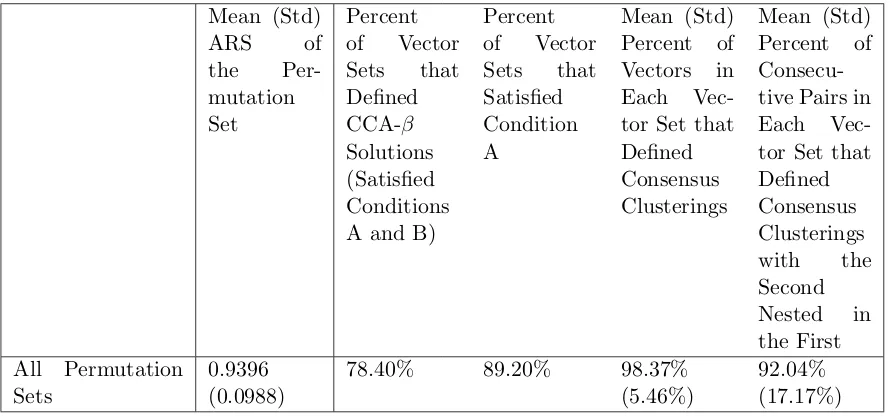
Figure 7.5 Percent of vector sets that defined CCA-β solutions by ARS. . . 79
Figure 7.6 Results for dlbcl50sample0-trial-3-partition4C-perm1 . . . 91
Figure 7.7 Difference in the Number of Consensus Clusterings Returned by CCA-ROPPPA and CCA-UPGMA . . . 97
Figure 7.8 Percent of ROPPPA Consensus Clusterings Also Returned by CCA-UPGMA . . . 98
Figure 7.9 Percent of UPGMA Consensus Clusterings Also Returned by CCA-ROPPPA . . . 99
Figure 7.10 Percent of ROPPPA Consensus Clusterings Also Returned by CCA-UPGMA and Percent of CCA-CCA-UPGMA Consensus Clusterings Also Re-turned by CCA-ROPPPA . . . 100
Chapter 1
INTRODUCTION
1.1
Gene Expression Analysis
With the advent of new technology, physicians and researchers have increasingly been able to extract and gain access to a great plentitude of gene related data. Analyzing such data has proven to be extremely useful to researchers in diagnosing various diseases and in discovering gene targeted disease therapies.
The most common type of data analyzed for these purposes is gene expression profile data. Gene expression is the process by which a gene expresses itself in protein synthesis. In genetics, it is how a genotype gives rise to an organism’s phenotype. The expression of a gene within a certain cell is typically analyzed by first measuring the amount of mRNA corresponding to that gene in the cell, and then using these mRNA levels to infer the expression of the gene. Gene expression analysis has become a very important tool in the study of diseases. For example, the expression levels of certain genes in a diseased patient may be higher or lower than the gene expression levels of a patient without this disease. The amount of pertinent genetic data in an organism or sample can range from 30,000 to 3 billion. Therefore data mining techniques are essential in decoding this overabundance of data.
for analysis is. That is why exploratory techniques which convey different facets of information about the data are ideal as well.
More specifically the underlying structure of gene expression data has been shown to exhibit a high level of clusterability. In a broad sense clusterability means that similar objects tend to group together in relatively homogenous groups called clusters. In terms of samples, this means that similar samples will group together in clusters displaying relatively similar gene expression data profiles. In terms of genes, this means that similar genes will group together in clusters having similar sample data. Because of this, cluster analysis is one of the most often used methods in extracting information about samples and genes.
Gene expression profiles are typically arranged in a real-valued expression matrix Φ = [φia]n,Fi=1,a=1 whereφia is the expression level of theath gene of samplei. The expression matrix can be used to either cluster the samples, using the F genes as features, or cluster the genes using thensamples as features. Clustering the samples, for instance, can assist in the diagnosis of disease and may even reveal disease subtypes, as studies have shown that clustering gene ex-pression profiles of patients with the same disease can often reveal two or more sub-types of this disease [Tam99]. Here it is assumed, that each patient has only one of these disease sub-types. Being able to identify and study the gene expression profiles of these disease sub-types can be helpful in the development of drugs or therapies aimed at eradicating these diseases. Alterna-tively, clustering the genes can help determine which genes are responsible for the development and progression of certain diseases and thus also play a pivotal role in the development of more intelligent drugs or therapies. Since the number of genes often greatly outnumbers the number of samples, we choose to focus on clustering the samples because our proposed methods, while useful for extracting pertinent additional information, are not as well equipped for handling data sets with a large number of objects as other methods are.
1.2
Gene Expression Clustering
There have been many suggested clustering algorithms that try to satisfy these gene expression related requirements. The k-means clustering algorithm [Llo82] has often been used due to its computational efficiency and simplicity. However, the initial placement of the centroids of the k-means algorithm will often produce different clustering results each time the algorithm is run. In addition, the user must preselect the number of clusters he or she wants in advance, which would thus require a preexisting knowledge of the data set. Finally, the k-means algorithm may be sensitive to noise [Sme02] [She01].
Self Organizing Map (SOM) [Koh84] approaches to clustering are also commonly used. SOM methods are beneficial in that they can provide insightful 2-d and 3-d visualizations of clustering results of a high dimensional data set. Herrero et al. [Her01] and Tamayo et al. [Tam99] suggest that SOM clustering methods are less sensitive to noise, however they are more sensitive to irrelevant data points. If there are too many irrelevant data points, such as genes with invariant patterns, then these data points will pervade many of the clusters.
Hierarchical clustering methods are also used very frequently in gene expression analysis. These methods are well adapted for data sets with nested clusters and can provide a dendrogram or tree graph that visually displays the results. Eisen et al. [Eis98] proposed an agglomera-tive hierarchical clustering algorithm known as UPGMA (Unweighted Pair Group Method with Arithmetic Mean) and used a particularly effective way of graphically displaying the clustering results. The drawbacks of hierarchical clustering methods are their high compuational complex-ity [Tam99] and their sensitivcomplex-ity to small perturbations [Tam99].
Graph-theoretic clustering algorithms are also commonly used. In respect to gene expression profile sample clustering, which is what we discuss in this paper, each sample is represented as a node in a graph. In some methods, a weighted edge is placed between each pair of samples. The weight between the samples is determined by a similarity metric. One such similarity metric would be the Euclidean distance between the gene expression levels of two samples. That is, the weight of the edge between samplesi and j would be the Euclidean distance between Φi∗
and Φj∗ [SS00] [XK01]. Other methods, simply place a 0 or a 1 weight on each edge based on
Although using a clustering algorithm to cluster gene expression data has proven to be very useful in unlocking hidden connections and information about disease and biological functions, there is no single algorithm which has proven to work best for all data sets as evidenced by the abundance of new clustering algorithms proposed each year. As shown above, each algorithm has its own strengths and weaknesses in their ability to meet the specialized needs of a comprehensive gene expression data analysis. Furthermore the exact goal of cluster analysis is at best a fuzzily defined notion. As there are a great number of clustering algorithms proposed in the literature, there are almost an equal amount of proposed objective functions aimed at optimizing and assessing the results of a clustering algorithm. However, defining the goal of clustering as one fixed objective function to optimize may in and of itself leave out a facet of information about the data that may also prove useful.
To further complicate the matter, many clustering algorithms like the k-means algorithm result in only a local optimal solution to the objective function they are trying to optimize. Many of these algorithms are initialized with random starting points and will thus produce different results because of this. Again, to say one local optimal solution is better than another is not necessarily the right mindset to take on in clustering as one local optimal result may provide some useful information that the other may not, and vice versa. Furthermore the question of how many clusters to consider is also a confounding factor in choosing the ’right’ clustering algorithm for gene expression analysis. While some algorithms require the user to preselect the resulting number of clusters in the clustering returned by the algorithm, other algorithms will return a clustering with a number of clusters chosen by the model. In either case, the question arises as to whether a resultant clustering with k clusters is the most informative. Would a resultant clustering withk−1 ork+ 1 clusters also provide useful information? In many cases the answer may be yes.
Because of all these confounding factors in conducting gene expression cluster analysis it is prudent for a researcher to consult the results of several different clustering algorithms run with different initializations and input parameters (if the algorithm allows it). However, the question of how to best amalgamate the results of all these algorithms is a difficult problem in and of itself.
1.3
Consensus Clustering
will call these differing clustering results theinput clusterings of a consensus clustering algo-rithm. Typically all the input clusterings are attained by clustering the same initial data set. Using the input clusterings as input, a consensus clustering algorithm returns a consensus clustering which achieves the most amount of consensus amongst the input clusterings.
Consensus clustering can be particularly beneficial in analyzing gene expression data as it has the power to create a consensus clustering result which may emphasize the strong input clustering results while downplaying weak or unwanted input clustering results. For instance, as we discussed in section 1.2, gene expression profile data is often noisy and the k-means algorithm is often sensitive to noise. Executing the k-means algorithm multiple times and using a consensus clustering algorithm to combine the results has the power to minimize the effect of this noise.
One of the drawbacks of using a consensus clustering algorithm, particularly for gene ex-pression analysis, is that it adds even more computational time to the analysis. Furthermore, since most consensus clustering algorithms only make use of the input clusterings and not the original data (used to create the input clusterings), information is inevitably lost in further processing. Useful information is also inevitably lost as most consensus clustering algorithms return only a single consensus clustering with no additional information such as the nested nature of the clusters.
In general, consensus clustering methods are comprised of two steps: 1. the generation step and 2. the consensus function step [VPRS11]. The generation step generates a set of input clusterings {π1, ..., πT} by executing one or more clustering algorithms a total of T times. Important questions to consider in this step are listed below.
1. Which clustering algorithms should be used?
2. If a clustering algorithm can produce different results, how many times should this algo-rithm be run?
3. If a clustering algorithm requires a preselected number of clusters k, how many clusters should be preselected?
4. Which subset of objects should be included in a given clustering algorithm (if not all)?
5. Which subset of object features should be used in the given clustering algorithm (if not all)?
The second step of a typical consensus clustering method uses a consensus function to find a consensus clustering that achieves the most consensus among the input clusterings. In the literature there are two main types of consensus function approaches: object co-occurrence and median partition [VPRS11].
1.3.1 Co-Occurence Consensus Clustering
The object co-occurrence approach is based on assigning an object to a cluster using a voting method which considers a.) the number of times a given object is assigned to a given cluster over all the input clusterings or b.) the number of times two given objects are assigned to the same (and different) clusters over all the input clusterings.
A common co-occurence consensus clustering approach first creates an n×n coassociation matrixS = [sij] where:
sij = 1 T
T X
t=1
δ(πt(oi), πt(oj)), (1.1)
where Π = {π1, ..., πT} is the set of input clusterings, δ(πt(oi), πt(oj)) = 1 ifoi and oj are assigned to the same cluster in the input clusteringπt, andδ(πt(oi), πt(oj)) = 0 ifoi and oj are assigned to different clusters inπt. After forming this matrix, typically an additional clustering algorithm is performed upon S, wheresij represents the similarity between oi and oj.
While there exists a great deal of literature surrounding co-occurence consensus clustering algorithms, we highlight the two following works in particular because a.) they use co-occurence consensus clustering algorithms for gene expression profile data and b.) they use a hierarchical clustering algorithm to recluster the co-association matrix. This is important for the purpose of comparison as the consensus clustering algorithm that we propose in this thesis is also a co-association consensus clustering algorithm, also uses hierarchical clustering algorithms, and also used on gene expression profile data.
In the first work, by Monti et al. [Mon03], a consensus based clustering algorithm is proposed for gene expression analysis that uses both hierarchical clustering and SOM clustering as the primary algorithms and perturbs the input data to create differing clustering results. They create a normalized weighted adjacency S = [sij] matrix between the samples, where sij is created using equation 1.1. They define their consensus score as P
i P
the quality of their algorithm. This consensus clustering algorithm is more so for the purpose of assessing clustering quality of the original clustering algorithm and whether the correct number of clusters were picked by this original algorithm. Furthermore, the results are subject to the the sampling method and the clustering algorithm used to reclusterS.
In the second work, by Kashef and Kamel [KK08], the researchers combine gene expression clustering results from both the k-means algorithm and the bisecting k-means algorithm to pro-duce a hierarchical clustering dendogram. Their proposed algorithm generates input clusterings as part of the consensus clustering algorithm so no time or information is lost and greater de-gree of consensus is reached. However, this consensus clustering algorithm only uses clustering results from the k-means and the bisecting k-means algorithms. It is not flexible in being able to provide a way to combine input clusterings generated from different clustering algorithms. They also do not provide a metric for assessing the consensus reached by the returned consensus clustering.
Other common consensus clustering methods that use object co-occurence consensus func-tions include relabeling and voting methods, coassociation matrix methods, graph and hyper-graph methods, information theory methods, finite mixture models, LAC algorithms, and fuzzy methods [VPRS11]. As with clustering algorithms, each consensus clustering algorithm has its merits. The benefit of object co-occurence methods is that they typically have a low compu-tational complexity, thereby allowing for the consensus clustering of larger data sets. However, they are lacking in mathematical rigor as they are not attempting to find an exact solution to an optimization problem. An exact optimization problem can give a quantitative score to assess how much overall consensus the consensus clustering had with the input clusterings, thereby yielding extra information about the data. Furthermore, its rich mathematical structure has the capability of being further exploited to yield extra information such as the nature of nested clusters and cluster closeness.
1.3.2 Median Partition Problem
The second main consensus clustering function is more mathematically rigorous as it selects a consensus clustering by solving an optimization problem which we define below.
π∗ =argmin | {z } π∈Π(O)
T X
t=1
Γ(π, πt) (1.2)
Researchers have proposed many functions for Γ, however one of the most widely used and studied functions is the symmetric difference distance function (or the Mirkin distance function) [Mir96].
Definition Let O ={o1, ..., on} be a set of objects and let π and π0 be two partitions (input clusterings) ofO. The Mirkin distancebetweenπ and π0 is defined as:
Γ(π, π0) =N01+N10, (1.3)
where N01 is the number of object pairs (oi, oj) for which oi and oj are clustered together in partition π0, but not in partitionπ and similarly N10 is the number of object pairs (oi, oj) for which oi and oj are clustered together in partition π, but not in partition π0.
In other words, the Median Partition Problem that uses the Mirkin distance seeks to min-imize the total disagreements between the each input clustering and the consensus clustering. Wakabayashi [Wak86] and Krivanek and Moravek [KM86] both proved in different ways that the Median Partition Problem with the Mirkin distance is NP-hard.
Filkov and Skiena [FS03] use heuristics of the Median Partition Problem to consensus-cluster gene expression profile data. They are able to consensus-consensus-cluster up to 1000 objects using their algorithms. They use the Rand index [Ran71] and proposed p-value to assess the agreement of the consensus clustering and all input clusterings. However, their algorithms are limited in providing only one clustering solution to the user.
Other common consensus clustering approaches which use the Median Partition Problem include Non-negative Matrix Factorization (NMF) methods, genetic algorithms, and kernel methods [VPRS11]. Unfortunately these methods rely upon a heuristic to solve the problem. Thus the theoretical rigor of the Median Partition Problem is lost to make way for higher data crunching capabilities.
1.4
IP Formulation of the Median Partition Problem with Mirkin
Distance
function.
min P
1≤i<j≤nwijxij
st xij+xjk−xik≤1 for 1≤i < j < k ≤n xij−xjk+xik≤1 for 1≤i < j < k ≤n
−xij +xjk+xik ≤1 for 1≤i < j < k ≤n xij ∈ {0,1} for 1≤i < j ≤n
xij = (
1 ifoi andoj are clustered together in the consensus clustering 0 otherwise
The objective function coefficients are defined as wij =wij−−wij+ where w+ij is the number of input clusterings that place oi and oj in the same cluster and wij− is the number of input clusterings that placeoi and oj in different clusters.
Note, another way to define wij is as follows:
wij = T X
t=1
(πt(oi), πt(oj)), (1.4)
where(πt(oi), πt(oj)) =−1 ifoiandojare assigned to the same cluster inπtand(πt(oi), πt(oj)) = 1 if oi and oj are assigned to different clusters inπt.
We call this the Grotschel Wakabayashi IP formulation (GWIP). We refer to the Grotschel Wakabayashi LP formulation (GWLP) as GWIP with relaxed binary con-straints.
The benefit of using the GWIP for consensus clustering is that it solves for an exact solution to the Median Partition Problem. The model has a rigorous mathematical structure, which in chapter 8 allowed us to discover a theoretical relationship to another existing problem in the literature in which there exist several fast heuristics.
However, to the best of our knowledge no researchers have attempted to extract additional information about the data using the mathematical structure of the model. Instead they choose to either solve the IP to optimality or accept a heuristic solution to the IP and conduct no further analysis.
A drawback of using the GWIP for the purpose of consensus clustering is that it has a relatively large number of variables and constraints, specifically 3 n3
constraints and n2
intractable.
Because of this, several researchers have proposed various techniques to increase problem tractability for larger n. Tushaus [T¨us83] introduces a branch and bound method that only works for small values of n. Wakabayashi and Grotschel [GW89] give a cutting plane method which is able to solve GWIP fornin the hundreds. These methods only discuss ways in which to make cuts or the branching schema more effective in the sense that as few LPs as possible have to be solved in order to get a binary optimal solution. However, what these methods do not take into account is that GWLP itself has a large number of constraints without any additional cuts or branch and bound restrictions and thus solving GWLP even once may prove to be an overly costly operation in and of itself.
Downing et al. [Dow10] propose a variety of constraint reduction techniques which increase efficiency in solving GWLP. Because the consensus clustering heuristic we propose in chapter 3 involves solving multiple linear programming formulations that are only slight modifications of GWLP, we employ some of these techniques in our proposed consensus clustering heuristic as well (chapter 3). These techniques are summarized below.
Solving the linear relaxation using a relaxed feasible region and then iteratively adding all of the constraints violated by the current optimal solution to the problem. An optimal solution to the original linear relaxation is reached when there are no more constraints violated by the current optimal solution to the problem.
Solving the linear relaxation using a relaxed feasible region and then iteratively addinga random sample of the constraints violated by the current optimal solution to the problem. An optimal solution to the original linear relaxation is reached when there are no more constraints violated by the current optimal solution to the problem.
Iteratively deleting constraints that correspond to basic variables in the dual of the cur-rent relaxed feasible region, provided that the optimal objective function value at the current iteration increased from the value of the optimal objective function in the previ-ous iteration. They explain why this method works in the literature.
the results of clustering the same original data set multiple times whereas the input clusterings Downing et al. to create [wij] are independent sets of categorical data. Thus our input clustering sets may have had an overall higher degree of consensus with one another than those used by Downing et al.
In addition, these researchers choose to focus less on producing an exact optimal solution and instead introduce a rounding schema which approximates the binary optimal solution in the event that the optimal solution to the linear relaxation is fractional. This rounding schema greatly reduces execution time in comparison to solving the GWIP by using branch and bound or cutting plane techniques. By using these efficiency improvements and approximate rounding techniques, Downing et al. [Dow10] were able to solve a consensus clustering data set of size n= 2048 within a reasonable amount of time. However, due to the fact that a rounding schema had to be introduced, this method is now only a heuristic to the MPP.
As discussed earlier, all of the research regarding the GWIP is concentrated at improving efficiency and reducing computational time in producing an optimal or near optimal solution to the GWIP. That is, the researchers produce one consensus clustering from GWIP and no further analysis is conducted on the data. This singular result can be a drawback to the purpose of gene expression analysis for the following reasons.
1. Not the Desired Number of ClustersFirst, the number of clusters obtained via the GWIP cannot be specified. Depending on the purpose of the analysis, researchers may have a predefined idea as to how many clusters they desire in the consensus clusterings. For instance, a data set we use in our numerical tests in chapter 7 consists of gene ex-pression profiles of four well established types of central nervous system tumors as well as gene expression profiles of normal cerebella tissue. For the purpose of diagnosis and classification it befits the researcher to desire each of the input clusterings as well as the consensus clustering to have five clusters. However, a set of input clusterings (each clustering having five clusters) was generated and GWLP returned a consensus clustering with eight clusters. While for the purpose of research and development this may actually provide useful information about further divisions of disease subtypes, for the purpose of quick disease classification this clustering with an excess of clusters may prove to be confusing. Thus it befits the researcher to have more consensus clustering result options, specifically consensus clustering results which yield fewer or greater than the number of clusters returned by GWIP.
nature. A singular clustering result returned by the GWIP does not reflect this nested nature. A hierarchical model which could convey how and when certain objects split away from other objects based on some metric of consensus cluster similarity would be beneficial in reflecting this, however no such models exist for this which use the GWIP.
1.5
Thesis Summary
In this thesis we slightly modify GWIP such that it still maintains the rich mathematical structure and reduced computation time techniques discussed in 1.4, but also allows for the discovery of nested consensus clusterings. In doing so, this thesis has five main contributions.
1. First we introduce a new cut, which we call a β-ratio cut. Using linear programming duality theory, we demonstrate a.) how our β-ratio cut is a natural extension of the cluster ratio cut [Yeh95] and b.) the rationale for why this cut is useful for the purpose of hierarchical consensus clustering.
2. Next we introduce a divisive hierarchical consensus clustering algorithm, which we call CCA-β that uses this β-ratio cut. Instead of one consensus clustering, this algorithm produces aset of nested consensus clusterings.
3. Then we introduce two heuristics for β, which we call OPPPA and CCA-ROPPPA. We call our methods CCA-OPPPA and CCA-ROPPPA heuristics of CCA-β because they will not always produce a set of nested consensus clusterings solutions that would have been a possible output of CCA-β. However, we show that whencertain condi-tions are satisfied by the results of our CCA-OPPPA and CCA-ROPPPA heuristics, they will produce a set of solutions that would have been a possible output of CCA-β. Our CCA-OPPPA and CCA-ROPPPA heuristics apply a parametric programming algorithm to a parametric LP formulation Pλ that we introduce (which is a slight modification of GWIP). While CCA-OPPPA uses an existing parametric programming algorithm [Ber96], CCA-ROPPPA uses a proposed parametric programming algorithm that is a slight mod-ification of this existing parametric programming algorithm.
5. Also using these sets of input clusterings generated from real gene expression profile data sets and artificial data sets, our fifth contribution will be to compare the CCA-ROPPPA heuristic to two other consensus clustering algorithms.
In chapter 2 we give some background needed in order to discuss our proposed consensus clustering algorithm. We define existing graph theoretic terms such as partitions, cuts, and a specialized type of cut, known as the minimum cluster ratio cut [Yeh95]. We also introduce and define our proposed cut, the β-ratio cut. We formally define the clustering and consensus clustering problem. We also discuss a widely used class of clustering algorithms, namely divisive hierarchical clustering algorithms. We discuss a specific type of divisive hierarchical clustering algorithm (DHCA) which uses ourβ-ratio cut. We call this DHCA-β and use it in our consensus clustering algorithm that we introduce in chapter 3. Finally in chapter 2 we define the Uniform Multicommodity Flow Problem [LR99], which we will use to show the rationale for β-cuts in chapter 8.
In chapter 3 we introduce our proposed consensus clustering algorithm CCA-β and its proposed heuristics, CCA-OPPPA and CCA-ROPPPA. Section 3.1 details how our proposed divisive hierarchical consensus clustering algorithm (CCA−β), uses DHCA-β (discussed in 2.3). In section 3.2 we introduce OPPPA and ROPPPA, our proposed heuristics for CCA-β.
CCA-OPPPA and CCA-ROPPPA apply a parametric programming algorithm to a para-metric LP formulation. In chapter 4 we introduce this parapara-metric LP formulation, which we call Pλ, and discuss various properties of it. In chapter 5 we introduce the parametric programming algorithms we apply to Pλ in CCA-OPPPA and CCA-ROPPPA. In section 5.1 we introduce notation and show various properties regarding Pλ. This terminology, which includes finding the dual ofPλ, is needed in explaining the parametric programming algorithms that we discuss in 5.2 and 5.3. In section 5.2 we discuss a parametric programming algorithm found in the lit-erature [Ber96], which we call OPPPA in this paper. Although the proof for why the algorithm works is too long to place in this dissertation, we briefly summarize how OPPPA works and give a few results related to the algorithm. The way that we present OPPPPA in 5.2 is made specific to our particular LP Pλ over the range [0, n2
], however OPPPPA as described in the literature can be applied to any parametric LP formulation.
than constraints. Thus we explain how we can use row generation techniques to more quickly solve the second LP in each iteration of OPPPA and use column generation techniques to solve the first LP in each iteration. By using the row generation techniques we introduce ROPPPA in 5.3.2 (using the column generation techniques are outside the scope of this dissertation, but are available for future research). Section 5.3.1 discusses the specific row generation techniques that we apply to the first LP in every iteration of ROPPPA. Section 5.4 discusses important proofs regarding OPPPA and ROPPPA.
In chapter 6 we show how our the results of our CCA-OPPPA and CCA-ROPPPA heuristics will produce CCA-β solutions if and only if the results satisfy certain conditions. The proofs we show in chapter 6 will be useful in chapter 8 when we demonstrate a.) how ourβ-ratio cut is a natural extension of the cluster ratio cut [Yeh95] and b.) the rationale for why this cut is useful for the purpose of hierarchical clustering.
In chapter 7, using real gene expression profile data sets and artificial data sets we create sets of clusterings for which we would like to find a consensus clustering(s). We then apply CCA-ROPPPA to these sets of clusterings and assess the frequency with which CCA-ROPPPA returns a set of consensus clusterings that could have been a result of CCA-β. Also in chapter 7, we compare CCA-ROPPPA to two other consensus clustering algorithms. We use the same real gene expression profile data sets and artificial data sets and the same sets of input clusterings created from these data sets. We then apply CCA-ROPPPA and the two other consensus clustering algorithms to these sets of clusterings and compare a.) the nature and quality of the consensus clusterings returned and b.) the execution times of the algorithms.
Specifically, in section 7.1 we discuss the two consensus clustering algorithms we will compare to CCA-ROPPPA. In section 7.2 we will discuss how we create input clustering sets that will be used as input for CCA-ROPPPA and the two other consensus clustering algorithms we test. In section 7.3 we give the specific computer, software, and LP solving options we used to execute all algorithms. In the appendix, for each of the input clustering sets that we created, we graphically display the results of the three consensus clusterings algorithms that used these input clustering sets as input. In section 7.4, we discuss how to interpret these graphs in the appendix. In section 7.5 we discuss the frequency with which CCA-ROPPPA returned a set of consensus clusterings that could have been a result of CCA-β. Finally in section 7.6 we compare CCA-ROPPPA to the two other consensus clustering algorithms we tested.
Chapter 2
BACKGROUND
In this chapter we introduce some important background to the problem which we intend to solve.
2.1
Graph Theory
2.1.1 Existing Graph Theoretic Terms
We first define some well-established graph theory terms. A graph G= (V, E) is defined by a set of vertices (nodes)V and a setE of pairs of distinct vertices called edges. We say that a set of disjoint subsets {V1, ..., Vr} of V is a partition (clustering) of a graph G= (V, E) if and only if V1∪...∪Vr = V and Vs∩Vt = φfor all s 6=t. We use the term cluster to refer to a disjoint subsetVs in a given partition (clustering){V1, ..., Vr}.
A complete graphis a graph in which all pairs of nodes are linked by an edge. We denote a complete graph with n nodes asKn. For a graph G= (V, E) whereU ⊂V,F ⊂E, and the vertices of each edge in F are also in U, then we say that H = (U, F) is a subgraph of G. A cliqueof a graph G= (V, E) is a subgraph ofG that is a complete graph.
Given a graph G= (V, E) we call a subset of edgesE(V1, ..., Vr) ∈E a clique partition if there is a partition {V1, ..., Vr} of V such that E(V1, ..., Vr) = ∪rs=1{(i, j) ∈ E|i, j ∈ Vs} and the subgraph induced by Vs is a clique for s = 1, ..., r. We say that the clique partition E(V1, ..., Vr) defines the partition {V1, ..., Vr}. We denote a clique partition that defines the partition{V1, ..., Vr}asE(V1, ..., Vr).
divide Ginto disjoint subgraphs G1(V1, E1), ..., Gr(Vr, Er). We denote such a cut C as follows:
C(V1, ..., Vr) ={(i, j)∈E|i∈Vs, j∈Vt, s6=t} (2.1)
where{V1, ..., Vr}is a partition ofV, for r≥2.
Note that a clique partition defines a cut C(V1..., Vr) =E/E(V1, ..., Vr).
If the graph G= (V, E) has edge weightsc:E →R, then we denote the value of the cut C(V1, ..., Vr) as the following (for r≥2):
|C(V1, ..., Vr)|=
X
(i,j)∈C(V1,...,Vr)
cij (2.2)
For notation purposes of this dissertation, we say that whenr= 1,C(V1) =C(V) and|C(V1)|=
|C(V)|= 0.
Yeh et al. [Yeh95] define the cluster ratio of a cutC(V1, ..., Vr) as:
RC(V1, ..., Vr) =
|C(V1, ..., Vr)|
P
1≤s<t≤r|Vs|˙|Vt|
(2.3)
forr≥2.
They define the minimum cluster ratio among all possible cutsC(V1, ..., Vr) of G(V, E) for all r≥2 as:
R∗C =minr≥2{RC(V1, ..., Vr)}. (2.4) A cutC∗(V1, ..., Vr) is aminimum cluster ratio cutof the graphG(V, E) if the cluster ratio of C∗(V1, ..., Vr) is equal to the minimum cluster ratio of G(V, E).
Yeh et al. [Yeh95] [SM90] also define theweighted cluster ratioof a cutC(V1, ..., Vr) as:
WC(V1, ..., Vr) = P
1≤s<t≤r
wst|C(Vs, Vt)| P
1≤s<t≤r
wst|Vs|˙|Vt|
(2.5)
forr≥2, wherew is a symmetric distance function. That is,wst>0 for all 1≤s < t≤r and wst+wtu≥wsu for all 1≤s < t < u≤r.
They define the minimum weighted cluster ratio among all possible cuts C(V1, ..., Vr) of G(V, E) for allr ≥2 as:
A cut C∗(V1, ..., Vr) is a minimum weighted cluster ratio cut of the graph G(V, E) if the weighted cluster ratio of C∗(V1, ..., Vr) is equal to the minimum weighted cluster ratio of G(V, E).
2.1.2 Proposed Graph Theoretic Terms
We say that a partition (clustering) {V1, ..., Vr} of a graph G(V, E) is nested in a
parti-tion (clustering) {U1, ..., Us} if {V1, ..., Vr} is the result of splitting one or more clusters in
{U1, ..., Us} into two or more clusters.
Given a graph G(V, E), a partition {U1, ..., Us}, and a partition {V1, ..., Vr} that is nested in{U1, ..., Us}, we define thecut difference of {V1, ..., Vr} and {U1, ..., Us} as
|C(V1, ..., Vr|U1, ..., Us)|=|C(V1, ..., Vr)| − |C(U1, ..., Us)| (2.7)
We propose the following terms which we can think of as an extension of the cluster ratio terms defined in 2.1.1. We discuss further in chapter 8 the rationale for why these terms can be thought of as extensions of the cluster ratio terms.
Definition Given a graph G(V, E), a partition {U1, ..., Us} of G, the cut C(U1, ..., Us), a par-tition {V1, ..., Vr} of G that is nested in {U1, ..., Us}, and the cut C(V1, ..., Vr) we define the β-ratio of C(V1, ..., Vr) given C(U1, ..., Us) as:
βC(V1, ..., Vr|U1, ..., Us) =
|C(V1, ..., Vr)| − |C(U1, ..., Us)|
P
1≤t<t0≤r|Vt|˙|Vt0| −P
1≤w<w0≤s|Uw|˙|Uw0|
. (2.8)
forr > s≥2.
Note that fors= 1, |C(U1, ..., Us)|= 0. The denominator of the ratio which is (the sum of the the multiplied cardinality of all pairs of clusters in{V1, ..., Vr}) - (the sum of the the multiplied cardinality of all pairs of clusters in {U1, ..., Us}). To remain consistent with this structure, when s= 1 we say that P
1≤w<w0≤s|Uw|˙|Uw0|=|U1|˙|φ|=|U|˙|φ|= 0.
Therefore when s= 1, theβ-ratio of C(V1, ..., Vr) given C(U1, ..., Us) is
βC(V1, ..., Vr|U1, ..., Us) =
|C(V1, ..., Vr)|
P
1≤t<t0≤r|Vt|˙|Vt0|
. (2.9)
We define theminimum β-ratio given C(U1, ..., Ur) among all possible cutsC(V1, ..., Vr) where{V1, ..., Vr}is nested in {U1, ..., Ur}as:
βC∗ =minr≥s{βC(V1, ..., Vr|U1, ..., Us)}. (2.10)
We say that a cut C∗(V1, ..., Vr) is a minimum β-ratio cut given C(U1, ..., Us) of a graph G= (V, E) if and only if
1. {V1, ..., Vr} is nested in{U1, ..., Us} and
2. theβ-ratio ofC∗(V1, ..., Vr) givenC(U1, ..., Us) is equal to the minimumβ-ratio cut given C(U1, ..., Us).
Note it also follows that whens= 1, a minimumβ-ratio cut givenC(U1, ..., Ur) is a minimum cluster ratio cut, and vice versa.
2.2
Clustering and Consensus Clustering
As summarized in the introduction, a the goal of a clustering problem is to find structure in an unlabeled set of objects. There are many different types of clustering algorithms which yield a variety of different output structures. A partition of objects can be one such type of output from a clustering algorithm. We use the phrase apartition-based clustering algorithm to refer to a clustering algorithm which yields a partition of the unlabeled set of objects. Our research deals with the question of how to best combine the partitions that are yielded as a result of executing one or more partition based clustering algorithms on thesame set of objects O={o1, ..., on}. With this in mind, we define the following notation.
We define aninput partition(orinput clustering)πof a set of objectsO={o1, ..., on}as a partition yielded by performing a partition-based clustering algorithm onO={o1, ..., on}. We define a partition-based consensus clustering algorithmas an algorithm which takes as input a set of input partitions (clusterings){πt}T
t=1(each created from the same set of unlabeled objects V = O = {o1, ..., on}) and outputs a new partition (clustering) π∗ = {V1, ..., Vr}. We refer to π∗ as a consensus clusteringof the set of input partitions (clusterings){πt}T
t=1. We use the term consensus cluster to refer to a disjoint setVs inπ∗ ={V1, ..., Vr}.
Finally we can measure the similarity between two clusterings π, π0 in a variety of different ways. One such way used by the literature is the RAND Index (RAND Score) [Ran71].
RAND Index (RAND Score)of π and π0 as
RAN D(π, π0) = N11+n N00 2
(2.11)
whereN11is the number of object pairs inO that are in the same cluster in bothπ and π0 and N00 is the number of object pairs in O that are in different clusters in both π and π0.
2.3
Divisive Hierarchical Clustering Algorithm
In our research we introduce a consensus clustering algorithm which uses a class of clustering algorithms known as divisive hierarchical clustering algorithms (DHCA) [Man08]. A DHCA takes a set of objects O ={o1, ..., on} and begins with a partition (clustering) p1 =O with all n objects in the same cluster. In each iteration at least one cluster in the current partition (clustering)pr−1 is selected and cut into at least two clusters creating a new partition (clustering)pr. This process is repeated until all objects are partitioned into singleton clusters. The result of a DHCA is a set of partitions (clusterings) {p1, ..., pR} where p1 is the set of all objects and wherepr is nested inpr−1 forr= 2, ..., R.
Which clusters are split and how they are split is dependent on the type of DHCA. A special type of DHCA is described as follows.
Divisive Hierarchical Clustering Algorithm with β-ratio cuts (DHCA-β)
Input: Set of objects O = V = {o1, ..., on} and S = [sij] where sij represents the similarity between objects oi and oj. Here we assume that as sij increases, similarity betweenoi and oj increases.
Output: A set of nested partitions ofV,{p1, ..., pR}.
1. Create a complete graph G= (V, E) with edge weightss:E→R. 2. Begin with a partitionp1 =V.
3. For each iteration r= 2, ..., Rcreate a partition pr such thatC(pr) is a minimumβ-ratio cut given C(pr−1).
for a given graph G= (V, E) and similarity matrix S it is the case that there exists only one minimum β-ratio cut in each iteration, then all implementations of DHCA-β will return the same result for this G= (V, E) and similarity matrix S.
2.4
Relevant Optimization Problems
Finally we introduce the following optimization problems found in the literature. They will be used in chapter 8 to a.) show how ourβ-ratio cut is a natural extension of the cluster-ratio cut and b.) demonstrate the rationale for our β-ratio cut.
Definition LetG= (V, E) be a graph, ρ be a set of commodities,C :E 7→R+ be a capacity function on the edges,S:V ×ρ7→R+be a supply function, andD:V ×ρ7→R+be a demand function. The multicommodity flow problem (MFP) [LR99] tries to construct flows for the commodities that satisfy the demand for each commodity at each vertex without violating the constraints imposed by the supply function and the capacity function.
Definition Auniform multicommodity flow problem (UMFP)[LR99] is a MFP where:
1. there is a separate commodity for each ordered pair of vertices (ρ=V ×V);
2. f half-units of commodity (i, j) must flow fromitojandf half-units of commodity (i, j) must flow fromj toifor each (i, j)∈E; and
3. f is maximized
We give two linear programming (LP) formulations for the UMFP in chapter 8. Finally we restate the Median Partition Problem with Mirkin distance here.
Definition LetO ={o1, ..., on}be a set of objects and let{πt}Tt=1 be a set of partitions (input clusterings) ofO. LetΠ(O) be the set of all possible partitions (input clusterings) that can be made fromO. Let Γ :Π(O)×Π(O)7→Rbe a similarity function. Then theMedian Partition Problem (MPP) [Lec94] returns a partition π∗ ∈Π(O) such that:
π∗ =argmin | {z } π∈Π(O)
T X
t=1
Γ(π, πt) (2.12)
Definition Let O ={o1, ..., on} be a set of objects and let π and π0 be two partitions (input clusterings) ofO. The Mirkin distancebetweenπ and π0 is defined as:
Γ(π, π0) =N01+N10, (2.13)
Chapter 3
PROPOSED CONSENSUS
CLUSTERING ALGORITHM AND
HEURISTICS
3.1
CCA-β
In this dissertation we introduce a co-occurence type of consensus clustering algorithm which uses DHCA-β. We call this proposed consensus clustering algorithm Divisive Hierarchical Consensus Clustering Algorithm with minimumβ-ratio cut (CCA-β). The algorithm is as follows:
Divisive Hierarchical Consensus Clustering Algorithm with a minimum β-ratio cut (CCA-β)
Input: Let Π ={π1, ..., πT} be a set of input clusterings of the set of objects O={o1, ..., on}.
Output: A set of nested consensus clusterings {p1, ..., pR}. 1. Create an×nco-association matrix C = [cij], where
cij = T X
t=1
δ(πt(oi), πt(oj)) (3.1)
δ(πt(oi), πt(oj)) = 1 ifoiandojare assigned to the same cluster inπtandδ(πt(oi), πt(oj)) = 0 if oi and oj are assigned to different clusters inπt.
There are different implementations of DHCA-β, thus there are different implementations of CCA-β.
Definition Let O = {o1, ..., on}. We say that a set of nested consensus clusterings Π =
{p1, ..., pR} is a CCA-β solution for {π1, ..., πT} if {p1, ..., pR} could have been returned by CCA-β where{π1, ..., πT} was the input.
In other words, p1 =O andC(pr) is a β-ratio cut givenC(pr−1) for r= 2, ..., R.
Note that if in each iteration of CCA-β given an input {π1, ..., πT} there exists only one β−cut, then all implementations of CCA-β will return the same result. In other words, there exists only one CCA-β solution for {π1, ..., πT}.
Clearly the most computationally taxing part of CCA-β is finding the β-ratio cut in each iteration. Our goal is to find efficient ways to determine a minimumβ-ratio cut in each iteration. In section 3.2 we propose two heuristics for CCA-β that use a parametric linear program model (PLP) that we introduce in chapter 4 and parametric programming algorithms which we introduce in chapter 5.
3.2
Heuristics for CCA-β
In this thesis we introduce two heuristics for CCA-β, given below. Both heuristics involve using a parametric LP formulation,Pλ, which we introduce in chapter 4 and one of two linear parametric programming algorithms (which we call OPPPA and ROPPPA) which we introduce in sections 5.2 and 5.3 respectively.
CCA-OPPPA Heuristic
Input:Let Π ={π1, ..., πT} be a set of input clusterings of the set of objects O={o
1, ..., on}. Output: A set of vectors {x∗(λ1), ...,x∗(λR)} where x∗(λr) is an optimal solution of Pλr for
r= 1, ..., R.
1. Create a co-association matrix C= [cij] , where
cij = T X
t=1
δ(πt(oi), πt(oj)) (3.2)
δ(πt(oi), πt(oj)) = 1 ifoiandojare assigned to the same cluster inπtandδ(πt(oi), πt(oj)) = 0 if oi and oj are assigned to different clusters inπt.
apply the parametric linear programming algorithm OPPPA (chapter 5.2) toPλ over the range [0, n2
].
CCA-ROPPPA Heuristic
Input:Let Π ={π1, ..., πT} be a set of input clusterings of the set of objects O={o1, ..., on}. Output: A set of vectors {x∗(λ1), ...,x∗(λR)} where x∗(λr) is an optimal solution of Pλr for
r= 1, ..., R.
1. Create a co-association matrix C= [cij], where
cij = T X
t=1
δ(πt(oi), πt(oj)) (3.3)
δ(πt(oi), πt(oj)) = 1 ifoiandojare assigned to the same cluster inπtandδ(πt(oi), πt(oj)) = 0 if oi and oj are assigned to different clusters inπt.
2. UseC= [cij] in the objective function of the proposed parametric LPPλ (chapter 4) and apply the parametric linear programming algorithm ROPPPA (chapter 5.3) to Pλ over the range [0, n2].
One thing to note is that the output of CCA-OPPPA and CCA-ROPPPA is a set of vectors
Chapter 4
PARAMETRIC LP MODEL
In this chapter we present our proposed parametric LP formulationPλthat is used in our CCA-OPPPA and CCA-RCCA-OPPPA heuristics. In section 4.1 we present the parametric LP formulation. In section 4.3 we discuss how to interpretPλ.
Because the feasible region of the GWLP (discussed in 1.4) is closely related to the feasible region of Pλ, many our results in section 4.3 rely upon results proven by Grotschel and Wak-abayashi [GW89] about the GWLP. Thus in section 4.2 we rewrite the GWLP, discuss how it is related toPλ, and give these results.
4.1
Parametric LP Model
P
λModified Grotschel Wakabayashi Linear Program Pλ Model
max P
1≤i<j≤ncijxij
st xij+xjk−xik ≤1 for 1≤i < j < k ≤n xij−xjk+xik ≤1 for 1≤i < j < k ≤n
−xij+xjk+xik≤1 for 1≤i < j < k ≤n P
1≤i<j≤nxij =M(λ)
xij ≥0 for 1≤i < j ≤n
Variables xij = (
1 ifoi and oj are clustered together in the consensus clustering 0 otherwise
Objective Function Coefficients
cij = T X
t=1
δ(πt(oi), πt(oj)), (4.1)
where Π ={π1, ..., πT}is a set of consensus clusterings, δ(πt(oi), πt(oj)) = 1 if oi and oj are assigned to the same cluster in πt and δ(πt(oi), πt(oj)) = 0 if oi and oj are assigned to different clusters inπt.
Parametric RHS M(λ) := n2−λ
4.2
Related GWLP Model
P
Our proposedPλ is related to the GWLP. We give the GWLP again in section 4.2.1. In section 4.2.2 we discuss how the GWLP is related to our Pλ. In section 4.2.3 we give several results that Grotschel and Wakabayashi prove about the GWLP which will help us in proving results about Pλ in section 4.3.
4.2.1 GWLP Model P
The GWLP (also in section 1.4) is shown again below.
Grotschel Wakabayashi Linear Program P (GWLP) Model
min P
1≤i<j≤nwijxij
st xij +xjk−xik ≤1 for 1≤i < j < k≤n xij −xjk+xik ≤1 for 1≤i < j < k≤n
−xij+xjk+xik≤1 for 1≤i < j < k≤n xij ≥0 for 1≤i < j ≤n
Variables xij = (
1 ifoi and oj are clustered together in the consensus clustering 0 otherwise
Objective Function Coefficients
wij = T X
t=1
(πt(oi), πt(oj)), (4.2)
where Π ={π1, ..., πT}is a set of consensus clusterings,(πt(oi), πt(oj)) =−1 ifoi andoj are assigned to the same cluster in πt and (πt(oi), πt(oj)) = 1 if oi and oj are assigned to different clusters inπt.
For the remainder of this thesis we denote the GWLP as P. We denote the feasible region of P as (P).
4.2.2 How (P) Relates to (Pλ)
4.2.3 Properties and Interpreting Solutions of P
The following are properties and lemmas about (P) proven by Grotschel and Wakabayashi [GW89].
Lemma 4.2.1 There is a one to one correspondence between the set of all clique partitions of
Kn= (V, E) and the set of all binary solutions of(P).
We can use this lemma to interpret binary solutions of (P). Interpreting Binary Solutions of (P)
Specifically, a binary x ∈(P) defines a clique partition E(V1, ..., Vr) of Kn = (V, E) (or equivalently a cut C(V1, ..., Vr) of Kn= (V, E) as follows:
C(V1, ..., Vr) ={(i, j)∈E|xij = 0} (4.3)
E(V1, ..., Vr) ={(i, j)∈E|xij = 1} (4.4)
Specifically, a binary x ∈ (P) defines a partition (consensus clustering) {V1, ..., Vr} of Kn= (V, E) as follows:
– By removing the edges in C(V1, ..., Vr) from E, we are left with a set of disjoint cliquesH1(V1, E1), ..., Hr(Vr, Er) of Kn.
– The partition (consensus clustering) is the set{V1, ..., Vr}.
Therefore, we say that ax∈(P) defines a (partition) consensus clustering pif and only if xis binary.
4.3
Properties and Interpreting Solutions of
P
λUsing the properties of P we can make a similar statement to that of lemma 4.2.1
Lemma 4.3.1 There is a one to one correspondence between the set of all clique partitions of Kn= (V, E) and the set of all binary solutions of(Pλ) for λ∈[0, n2
].
Proof Suppose there exists a clique partition E(V1, ..., Vr) (or cutC(V1, ..., Vr)) of
toC(V1, ..., Vr). Specifically xij = 0 if (i, j)∈C(V1, ..., Vr) andxij = 1 otherwise. Because Kn is a complete graph, then |E|= n2
and
|{(i, j)∈E|(i, j)∈/ C(V1, ..., Vr)}|= n2
− |C(V1, ..., Vr)| If we letλ=|C(V1, ..., Vr)|, then it follows that
P
1≤i<j≤nxij =P(i,j)∈C(V1,...,Vr)xij +
P
(i,j)∈/C(V1,...,Vr)xij
=P
(i,j)∈/C(V1,...,Vr)xij
= n2
− |C(V1, ..., Vr)| = n2−λ
Thus there exists aλ∈[0, n2] such that x∈(Pλ). Thus C(V1, ..., Vr) corresponds to a binary solution in (Pλ).
Now suppose there exists a binary x∈(Pλ). Because (Pλ) = (P)∩ {x|P
i<jxij =M(λ)}, then it must be the case thatx∈(P). Thus by lemma 4.2.1, there exists a clique partition that corresponds to x.
Because of lemma 4.3.1 we can interpret binary solutions of Pλ the same way as we did for binary solutions ofP.
Interpreting Binary Solutions of (Pλ)
Specifically, a binary x(λ) ∈(Pλ) defines a clique partition E(V1, ..., Vr) ofKn = (V, E) (or equivalently a cutC(V1, ..., Vr) of Kn= (V, E)) as follows:
C(V1, ..., Vr) ={(i, j)∈E|x(λ)ij = 0} (4.5)
E(V1, ..., Vr) ={(i, j)∈E|x(λ)ij = 1} (4.6)
Specifically, a binaryx(λ)∈(Pλ) defines a partition (consensus clustering){V1, ..., Vr}of Kn= (V, E) as follows:
– By removing the edges in C(V1, ..., Vr) from E, we are left with a set of disjoint cliquesH1(V1, E1), ..., Hr(Vr, Er) of Kn.
– The partition (consensus clustering) is the set{V1, ..., Vr}.
Furthermore if x(λ1) ∈ (Pλ1), ...,x(λR) ∈ (PλR), then we can also say that a set
{x(λ1), ...,x(λR)}defines a set of (partitions) consensus clusterings {p1, ..., pR}if and only if each vector in the set is binary.
Next, (using the definition in 3.1) ifx(λ1)∈(Pλ1), ...,x(λR)∈(PλR), then say that a set
{x(λ1), ...,x(λR)} defines a CCA-β solution for {π1, ..., πT} if and only if
– {x(λ1), ...,x(λR)} defines a set of consensus clusterings{p1, ..., pR} and
– {p1, ..., pR} is a CCA-β solution for {π1, ..., πT}
Finally, if CCA-OPPPA (CCA-ROPPPA) is applied to an input clustering set{π1, ..., πT}
and returns the set of vectors {x(λ1), ...,x(λR)}, then we say that CCA-OPPPA (CCA-ROPPPA)returned a CCA-β solution for{π1, ..., πT}if and only if{x(λ1), ...,x(λR)} defined a CCA-β solution for {π1, ..., πT}.
Chapter 5
Parametric Programming
Algorithms
In this chapter, we present and discuss the parametric linear programming algorithms that are used in our CCA-OPPPA and CCA-ROPPPA heuristics. In general, the goal of a parametric linear programming algorithm is to determine how the optimal solution and the optimal objec-tive function value of a given parametric LPLP(θ) change asθis perturbed over some interval whereLP(θ) is feasible. A typical result that can be returned from a parametric programming algorithm is a continuous set of solutions {x∗(θ)} that are optimal in LP(θ).
For the purpose of this thesis, the goal of applying a parametric linear programming al-gorithm specifically to Pλ over λ ∈ [0, n2
] is to return a discrete set of vector solutions
{x∗(λ1), ...,x∗(λR)} (that are optimal in Pλ1, ..., PλR respectively) that defines a CCA-β
so-lution. Thus the two parametric programming algorithms we present in this chapter will only return a finite set of solutions. Sections 5.2 and 5.3 will discuss in further detail which solutions are chosen in the algorithms.
In section 5.2 we discuss the parametric programming algorithm that we use in our CCA-OPPPA heuristic. This parametric programming algorithm is found in the literature [Ber96] and we call it OPPPA in this dissertation. In section 5.3 we propose the parametric programming algorithm that we use in our CCA-ROPPPA heuristic. This parametric programming algorithm is a modification of OPPPA and we call it ROPPPA.
arenecessary conditions for a set of vectors to define a CCA-β solution.
5.1
Parametric Programming Algorithm Notation and
Proper-ties
5.1.1 Parametric Programming Algorithm Notation
First, in section 5.1.1 we introduce some notation that we will use in explaining the parametric programming algorithms that we introduce in sections 5.2 and 5.3. In order to use these para-metric programming algorithms we must have Pλ satisfy some properties. In section 5.1.2 we show and prove these properties.
5.1.1.1 Primal Formulations
Parametric Primal Problem:We definePλ ={maxc0x|Ax≤b,e0x= n2
−λ,x≥0}
as the primal ofPλ (matrix notation) with parameterλfor allλ∈[0, n2
]. In this formula-tion we have c0 = [c12, c13, ..., c1n, c23, c24, ..., cn−1,n], x0 = [x12, x13, ..., x1n, x23, x24, ..., xn−1,n], e0 = [1,1, ...,1], and b = [1,1, ...,1]. Written another way, we writePλ as:
max P
i<jcijxij
st a(ijkh)0x≤bijk(h) ∀1≤i < j < k≤n, h= 1,2,3 P
i<jxij = n2
−λ
xij ≥0 ∀1≤i < j≤n
whereb(ijkh)= 1 for all 1≤i < j < k ≤nandh= 1,2,3; anda(ijkh)0 is a row vector of length n
2
where
– a(1)ijk0x≤b(1)ijk represents the constraintxij+xik−xjk ≤1 – a(2)ijk0x≤bijk(2) represents the constraintxij−xik+xjk ≤1 – a(3)ijk0x≤b(3)ijk represents the constraint−xij+xik+xjk ≤1.
Parametric Primal Problem (Standard Form):We define ¯Pλ ={maxc0x|Ax+z= b,e0x= n2
¯
c0 = [c0|0, ...,0],x¯0 = [x0|z0],z0 = [z(1)123, z123(2), z123(3), ..., z(1)n−2,n−1,n, zn(2)−2,n−1,n, zn(3)−2,n−1,n], and
¯ A=
" A I e0 00
#
Also in this formulation we define the right-hand-side (RHS) vector of ¯Pλ as the function b(λ) =b−λ∆bwhere b= [b0| n2
]0 and∆b= [0,0, ...,0,1]0. Written another way, we write ¯Pλ as:
max P
i<jcijxij
st a(ijkh)0x+z(ijkh)=b(ijkh) ∀1≤i < j < k ≤n, h= 1,2,3 P
i<jxij = n 2
−λ
xij ≥0 ∀1≤i < j ≤n
zijk(h) ≥0 ∀1≤i < j < k ≤n, h= 1,2,3
wherea(ijkh)0 is a row vector of length n2 where
– a(1)ijk0x+z(1)ijk=b(1)ijk represents the standard form constraintxij+xik−xjk+z (1) ijk= 1, – a(2)ijk0x+z(2)ijk=b(2)ijk represents the standard form constraintxij−xik+xjk+z(2)ijk= 1,
and
– a(3)ijk0x+z(3)ijk=b(3)ijk represents the constraint−xij+xik+xjk+z (3) ijk= 1.
Parametric Primal Feasible Region:We define (Pλ) and ( ¯Pλ) as the feasible regions of Pλ and ¯Pλ respectively for allλ∈[0, n2].
Parametric Primal Solutions: We use the notation x(λ) or ¯x(λ) := [x(λ)0|z(λ)0]0 to represent a solution of Pλ and ¯Pλ respectively.
Parametric Primal Optimal Solutions: We define Pλ∗ and ¯Pλ∗ as the set of optimal solutions ofPλ and ¯Pλ forλ∈[0, n2
].
5.1.1.2 Dual Formulations