Towards an Optimized Internet Backbone Network.

ABSTRACT

MA, XUEZHOU. Towards an Optimized Internet Backbone Network. (Under the direction of Khaled Harfoush.)

The explosive growth of traffic demand, fueled by the expansion of the Internet in reach and capacity, imposes severe stress on backbone networks. A tier-1 Internet Service Provider (ISP) like AT&T delivers more than 7 petabytes of data per day through its backbone fabric where as little as 1% higher traffic loss will incur several terabytes of retransmissions, almost equivalent to the daily load of a medium-sized regional network, and billions of dollars are spent annually on infrastructure construction and equipment upgrade to satisfy the increasing bandwidth requirements. An optimized design for Internet backbone networks thus benefits both service providers and Internet users worldwide.

Despite the large body of research targeted at optimizing backbone networks, it remains challenging to identify the actual major factors driving the design and create a realistic and tractable model with appropriate design metrics. The development of networking technologies further complicates the problem by continuously shifting the bottleneck factors from some elements to others. Moreover, with the advent of the concept of green Internet, legacy models aimed at maximizing the throughput are tuned to a new energy-smart perspective aimed at minimizing the energy footprint. Such rapid evolution of backbone networks leaves many critical issues unsolved, inspiring more investigations and discussions in the research community.

© Copyright 2012 by Xuezhou Ma

Towards an Optimized Internet Backbone Network

by Xuezhou Ma

A dissertation submitted to the Graduate Faculty of North Carolina State University

in partial fulfillment of the requirements for the Degree of

Doctor of Philosophy

Computer Science

Raleigh, North Carolina 2012

APPROVED BY:

Rudra Dutta Harilaos Perros

Douglas Reeves Khaled Harfoush

DEDICATION

This dissertation is dedicated to my wife and my parents who have supported me all the way since the beginning of my studies. This dissertation is also dedicated to my grandmother who

BIOGRAPHY

ACKNOWLEDGEMENTS

TABLE OF CONTENTS

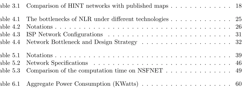
List of Tables . . . vii

List of Figures . . . .viii

Chapter 1 Introduction . . . 1

Chapter 2 Related Works. . . 4

2.1 Network Physical Topology Design . . . 4

2.2 Network Virtual Topology Design . . . 5

2.3 Network Robustness and Energy Efficiency . . . 6

Chapter 3 HINT: A Realistic Physical Topology Model . . . 8

3.1 Network Design Factors . . . 9

3.1.1 Traffic Model . . . 10

3.1.2 Economics and Geographical Constraints . . . 10

3.1.3 Quality of Service . . . 11

3.1.4 Survivability . . . 12

3.2 Problem Formulation . . . 12

3.3 Our Heuristic Algorithm . . . 15

3.4 Performance Evaluation . . . 16

3.5 Summary . . . 20

Chapter 4 The Efficacy of WDM Virtual Topology Design Strategies . . . 21

4.1 WDM Virtual Topology Design Factors . . . 22

4.2 A Bottleneck-Oriented Design . . . 26

4.2.1 Problem Definition and Assumptions . . . 26

4.2.2 Key Idea . . . 26

4.2.3 Algorithmic Details . . . 30

4.3 Performance Evaluation . . . 31

4.4 Summary . . . 34

Chapter 5 Towards a Robust and Green Internet Backbone Network . . . 35

5.1 Network Architecture and Power Consumption Model . . . 36

5.2 Network Robustness to Traffic Spikes . . . 38

5.3 Problem Statement . . . 39

5.3.1 Terminology . . . 39

5.3.2 Problem Formulation . . . 40

5.4 A Two-Phase Heuristic . . . 41

5.4.1 Key Idea . . . 41

5.4.2 Phase I – Virtual Graphs with Bounded Congestion . . . 42

5.4.3 Phase II – Traffic Routing with Optimized Power Usage . . . 44

5.5 Performance Evaluation . . . 45

Chapter 6 Traffic Concentration for a Green Internet . . . 50

6.1 Router Cooling System and Power Consumption Model . . . 51

6.2 Problem Statement and Heuristic Algorithm . . . 54

6.2.1 MILP Formulation . . . 54

6.2.2 Key Idea . . . 55

6.2.3 Heuristic Algorithm . . . 57

6.3 Performance Evaluation . . . 58

6.4 Summary . . . 60

Chapter 7 Conclusion . . . 61

LIST OF TABLES

Table 3.1 Comparison of HINT networks with published maps . . . 18

Table 4.1 The bottlenecks of NLR under different technologies . . . 25

Table 4.2 Notations . . . 26

Table 4.3 ISP Network Configurations . . . 31

Table 4.4 Network Bottleneck and Design Strategy . . . 32

Table 5.1 Notations . . . 39

Table 5.2 Network Specifications . . . 46

Table 5.3 Comparison of the computation time on NSFNET . . . 49

LIST OF FIGURES

Figure 3.1 Published network map: Level3 network [5]. . . 9

Figure 3.2 An illustration of traffic model in a 3-node graph with δ1 = 1, δ2 = 2, and δ3= 4 (left). A more compact representation of the traffic flows between nodes (middle); A symbolic representation of flows(right). . . 11

Figure 3.3 The basic idea of our physical topology design. . . 13

Figure 3.4 Physical topology designs for 13-link Abilene network. (a) optimizing only cost Cl (γ = 10), (b) optimizing only performance Cd (γ = 0.1), (c)optimizing both cost and performance (γ = 1) without survivability constraint, (d) optimizing both cost and performance (γ = 1) with sur-vivability constraint . . . 17

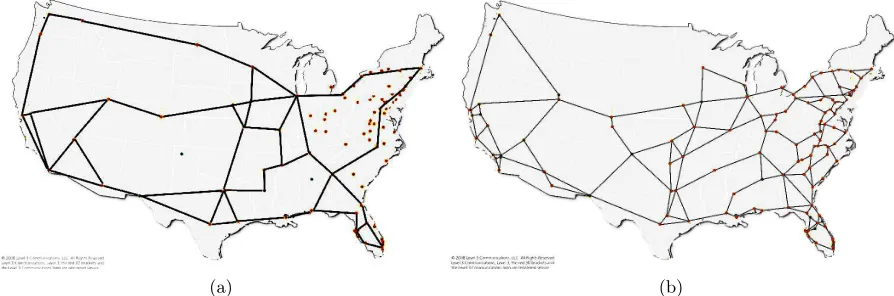
Figure 3.5 HINT results for (a) AT&T and (b) Level3. Shaded background image is from [5] with permission to use. . . 18

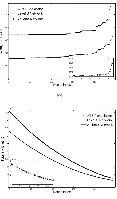
Figure 3.6 The change of (a) total link length Cl and (b) average delayCd through HINT optimization. . . 19

Figure 4.1 Virtual topology maps. (a) NLR [7] and (b) Sprint [44]. Note that each edge in the maps may represent multiple parallel lightpaths. . . 22

Figure 4.2 A typical structure of the backbone PoP node. The OXC node structure can be obtained by removing the routers from this figure. . . 23

Figure 4.3 Physical topology for Sprint network [44]. Each edge in the graph repre-sents optical fibers. The PoP nodes are marked with green box. . . 24

Figure 4.4 Comparison of OXCs and routers in term of switching capacity. Informa-tion in this figure is collected from [41] and manufacturer web sites based on data from 2006. . . 24

Figure 4.5 An illustration of preferred lightpath layout. (a) Router capacity is the bottleneck; (b) Wavelength capacity is the bottleneck; (c) Both router and wavelength capacity are bottlenecks. . . 28

Figure 4.6 Comparison of BOA with two other design approaches in terms of (a) the maximum lightpath utilization, (b) the maximum node utilization, (c) the network throughput. . . 33

Figure 5.1 Architecture of an IP-over-WDM backbone network. . . 37

Figure 5.2 Two virtual topology designs on a five-node two-wavelength network (a) minimizing the maximum utilization; (b) minimizing the power consump-tion. Traffic flows that traverse each lightpath/node are exhibited in the figures. . . 40

Figure 5.3 Variants of traffic routings in Figure 5.2 with the same virtual graph. (a) a variant of Figure 5.2 (a) minimizing the power consumption, (b) a variant of Figure 5.2 (b) minimizing the maximum utilization. . . 41

Figure 5.4 Design strategies of two factors on solving each subproblem. . . 42

Figure 5.5 Power consumption incurred by SP and non-SP routings. . . 44

Figure 5.7 Total power consumption. (a) NLR and (b) NSFNET. . . 47

Figure 5.8 The maximum utilization. (a) NLR and (b) NSFNET. . . 48

Figure 6.1 Architecture of a hybrid router cooling system. . . 52

Figure 6.2 Realistic router power consumption. . . 53

Figure 6.3 Comparison of two traffic routing scenarios: (a) traffic balancing, (b) traf-fic concentration. . . 55

Figure 6.4 Physical topology maps. (a) NSFNET and (b) AT&T. . . 58

Chapter 1

Introduction

The Internet is a global system of interconnected networks in which a large number of private, public, business, and government networks of local to global scope are linked. An Internet backbone service provider maintains Points of Presence (PoPs) in different locations, typically in densely populated areas, and interconnects these PoPs by means of fiber links, creating a backbone network. Backbone networks interconnect to construct a large network with global reach. In order to gain access to the Internet, edge networks or customers connect to the Internet backbone either directly or through regional networks, which are themselves connected to the backbone.

The explosion of the Internet in reach and capacity is fueled by a significant boost of net-working technology at the backbone. Conventionally, each fiber link carries a single signal. Huge optical bandwidth, which is in the order of Tbps, was wasted due to the limited speed of elec-tronic devices at fiber ends. The use of Wavelength Division Multiplexing (WDM) compensates this mismatch by dividing fiber bandwidth into tens ofwavelengths each able of carrying traffic in the order of Gbps. A virtual channel,lightpath, can be established between PoPs by using one wavelength on each link along the path. Once established, it delivers information transparently such that the signal cuts through intermediate PoPs without electronic switching. The set of all lightpaths then forms a virtual graph on top of the backbone infrastructure,physical topology. Routing and Traffic Engineering (TE) mechanisms are handled over these virtual channels.

Despite the large body of research targeted at optimizing backbone networks, it remains challenging to identify the actual major factors driving the design and create a realistic and tractable model with appropriate design metrics. The development of networking technologies further complicates the problem by continuously shifting the bottleneck factors from some elements to others. For example, previous research has repeatedly minimized the link/channel utilization to increase the network throughput, while newly deployed infrastructures can support as many as 64 wavelengths on a single fiber with 40 Gbps bandwidth for each. That is several order of magnitude larger than the switching capacity of core routers in the market, implying that the routers are more likely to be the bottleneck in modern networks. Moreover, given that a sizable fraction of total electricity supply in the U.S. is devoured by backbone infrastructure, the concept of green Internet has been highlighted recently. Legacy models aimed at maximizing the throughput are tuned to a new energy-smart perspective aimed at minimizing the energy footprint. Such rapid evolution of backbone networks leaves many critical issues unsolved, such as how to balance the throughput and energy requirements, inspiring more investigations and discussions in the research community.

In this dissertation, we study the WDM backbone networks from the bottom up, starting with physical topology and then extending to virtual topology and traffic routing. We make the following contributions.

1. We present a physical topology model, HINT, to determine the number and the choice of constituent fiber links. Previous models based on the optimization of deployment cost lead to the results not matching the real graphs, while HINT captures the physical de-sign principles including cost, performance, resilience and geographical constraints, and it considers the problem as a tradeoff among all feasible meshes that yield best performance for a given budget. HINT achieves a similarity of more than 90% with the published ISP structures.

2. Existing virtual topology models optimize predetermined objective functions of interest. They are highly dependent on the network context, and a model that fits one network can perform poor for others. Our heuristic approach, BOA, abstracts the individual design objectives by iteratively identifying the bottleneck elements and setting up suitable virtual channels accordingly. BOA is plug-and-play and averages 28% higher throughput than existing models in all tested networks with different traffic demands and technologies. 3. In virtual topology design, a model aimed at maximizing energy savings by aggregating

power usage for common traffic demand, while accommodating traffic fluctuations. The proposed heuristic matches the optimality of both factors within 10%, while reducing the computation time to less than 40 minutes compared to 22 hours for optimal solutions. 4. Existing backbone traffic routing schemes that minimize the aggregate router power usage

are mislead by ignoring the impact of cooling consumption. We show that the actual router power spectrum is polynomial in traffic demand and increases rapidly when the router is loaded. We compare the efficacy of two distinct routing philosophies, traffic aggregation vs. traffic balancing, and make a case that mitigating network bottlenecks, rather than creating ones, can save at least 25% energy. Our conclusions challenge the common wisdom about the merit of load concentration strategies.

Chapter 2

Related Works

In general, there are two main approaches to network topology design, namelystatistic modeling and optimization. Statistic modeling depends on an emerging picture of the large-scale statis-tical properties of networks which are acquired through careful collection and interpretation of topology-related measurements [50, 63]. Measured properties are used in designing and testing new topologies. Optimization techniques [11,24,32,33,59,60] attempt to find the optimal design result for a pre-determined objective function with subject to network resource constraints. The objective function is formalized to reflect metrics of interest. Since statistic modeling represents an average feature map, design models aiming at individual networks mostly use optimization approach. The optimization problem is typically casted as a Linear Programming (LP) prob-lem [24, 60] and solved using software packages such as Cplex for small sized cases. To make it tractable for real networks, heuristic algorithms are needed to obtain the approximate or near-optimal solutions.

2.1

Network Physical Topology Design

Unfortunately, existing models can not justify their results by comparing to real ISP networks. The cost and survivability may not be the only factors in determining network structure.

The problem of designing a physical topology to optimize the number of wavelengths is known to be NP-hard [33]. Minimizing the total link length without ensuring a 2-connected graph is equivalent to searching for the minimum spanning tree. The complexity is O(V2) (V is the number of nodes) by using Prim’s algorithm. Computational complexity for examining two-connectivity grows exponentially with the size of the network [26]. Heuristic algorithms are proposed for obtaining a survivable network with minimum cost. Some studies [26, 33] use a constructing algorithm starting with a minimum spanning tree and then adding the links which render maximum improvement on the objective. Others [13, 60] rely on greedy approaches to exchange the configurations of neighboring nodes during each iteration.

2.2

Network Virtual Topology Design

For years, WDM virtual topology design has been formulated to maximize the network through-put subject to constraints on network resources. Many popular design metrics have been con-sidered and each of them was shown optimal for only certain networks or scenarios. In [13], the packet hop distance is minimized since the average hop distance is inversely proportional to the network throughput, when traffic demand is balanced across the network. In [31], themaximum link utilization is minimized because an overall throughput scale-up was often limited by over-congested links. In [53], a virtual layout with the minimum usage of network resources (e.g., wavelengths) is selected to fight against traffic fluctuations. In [41], reducing thedemand delay product (i.e., the product of traffic rate and end-to-end queuing delay), equivalent to reducing the amount of data “on the line”, is used to maximize the network throughput. In the case router ports are scarce resources, maximizing thechannel load by grooming low-rate flows into one channel is shown more appropriate in [66]. Despite the rich literature in this area, relying on one objective function in all cases is expected not to lead to the maximum throughput in all networks independent of bottleneck elements in these networks.

2.3

Network Robustness and Energy Efficiency

Traffic dynamics are extensively studied and mitigated by by optimizing traffic routing through Traffic Engineering (TE) techniques. Early efforts [22, 23] have investigated the routing opti-mization problem in the case of a single traffic matrix. In [23],Gallager proposes a distributed gradient-based algorithm to solve the problem by changing the routing variables. The work in [22] approximates the link utilization as piece-wise linear functions, and solves the problem using LP. To emulate the different possible traffic spikes, the literature is formalized to minimize themaximum link utilization (MLU) in the presence of multiple traffic matrices (Surprisingly, very little work has been found on minimizing the maximum router utilization). In [65], Zhang et al.consider a set of representative traffic patterns and search for an optimal routing to mini-mize the MLU over all representative patterns. In [57], the authors distinguish normal operation and link congestion and propose a heuristic to cope both traffic spikes and common demand. While there is a large body of research in the TE field, the proposed solutions do not apply directly to the WDM virtual topology design due to the lack of consideration to the optical layer.

Energy concerns are highlighted recently. Research efforts in WDM network design have shifted to network power models and LP formulations in order to minimize energy footprint [15, 28, 48, 55]. In [48], an objective function that includes the power consumption of routers, transponders, and amplifiers is minimized for given traffic demand. Two heuristics, one with all routers bypassed by the virtual channels and the other with no router bypassed, are shown in [48] to find near-optimal virtual designs. In [28], the authors consider the network power model which consists of electronic routers and optical switches, and propose a flow-based and a interface-based formulations to measure the overall power usage. However, as far as we know, none of existing models attempt to handle both energy savings and network performance.

Chapter 3

HINT: A Realistic Physical

Topology Model

The physical topology of a network is expressed as a graph G = (V, E), which identifies the physical layout of devices in the network,V, together with the way devices are interconnected through actual cables, E. In this chapter, we investigate the physical topology of Internet backbone networks, in whichV is the set of PoPs andE is the set of fiber links interconnecting them. Specifically, our aim is to answer the following question: Given the POP locations of a service provider, enabling technologies and traffic demands, how should the service provider lay

out fiber links and what are the driving forces behind this layout?

Identifying the actual major factors driving the design of the physical topologies of Internet backbone networks, and understanding how they interact, is essential since a practical design 1) can reduce the capital investment for ISPs, 2) directly impacts higher layer protocols and applications [13], and 3) provides critical support for Internet researchers in need of practical network models. Most research on physical topology design has focused on deployment cost [24, 33,59,60]. Later studies pointed out that due to technological, cost and performance constraints, Internet backbone networks have a sparse meshstructure [11, 32] – Refer to Figure 3.1 for an example. The study in [11, 32], however, does not explain how a sparse mesh is constructed, i.e., which links are established.

Figure 3.1: Published network map: Level3 network [5].

be NP-hard. We thus introduce a polynomial time heuristic algorithm, HINT, to determine the number and the choice of the constituent links. The efficacy of HINT is established in com-parison with the published maps of three major scientific and commercial backbone networks: Internet2 Abilene, AT&T domestic express backbone, and Level3 network. Our results reveal that taking performance and resilience into consideration is necessary to emulate real backbones. The HINT heuristic yields a similarity of more than 90% with the published structures.

The rest of this chapter is organized as follows. In Section 3.1, we discuss the physical topology design factors. In Section 3.2 and 3.3, we formulate the optimization problem and the HINT heuristic. In Section 3.4, we compare HINT results with the published ISP networks. Summary is in Section 3.5.

3.1

Network Design Factors

3.1.1 Traffic Model

The demand for Internet service is a major driving force in network design. [18] indicates that the average aggregate traffic between two nodes (PoPs) can be approximated by their population. Since backbone nodes are usually located at major cities, two cities with higher population are likely to exchange more traffic. We thus rely on the traffic model introduced next.

Let δi be the population of node vi. Suppose vi exports δi (in traffic units) to G and imports/downloads δi from G. The imported δi units are downloaded from nodes of G in proportion to their δ values. The exported δi units are uploaded to all other nodes also in proportion to their δ values. Let σ = P|V|

i=1δi. Then a node vi uploads a fraction δ_σj of its δi traffic units to nodevj and downloads a fraction δ_σi ofδj fromvj. Note that this model generates the same amount of traffic in both directions (originating at vi and destined for vj and vice versa). The end-to-end traffic between vi and vj can be expressed as:

λij =δi δj

σ +δj δi

σ = 2δiδj

σ (3.1)

Refer to Figure 3.2 for an example. In Figure 3.2 (left), a directed link from a node vi to node vj is annotated with the traffic from vi to vj. Figure 3.2 (middle) provides a more compact representation in which we summed up the traffic units in both direction instead of distinguishing them. Figure 3.2 (right) then shows the equivalent traffic carried on fiber links. Self cycles are not considered in our model as they do not affect performance in Section 3.1.3. Note that the sum of the traffic units over all links in this representation equalsσ as expected. Also,λij in our traffic model is proportional to the product ofδi andδj. At the same time, the aggregate traffic at one node (e.g.,P

jλij for nodevi) keeps linear form ofδ. That differs from the gravity model in [47].

3.1.2 Economics and Geographical Constraints

Cost plays an important role in determining the physical topology. The cost for constructing a backbone network has many facets. Some costs areone-time infrastructure investments such as purchasing fibers and optical switches, digging and installing fibers underground. Other costs arerecurring such as hiring personnel to run the equipment and the associated overhead.

Figure 3.2: An illustration of traffic model in a 3-node graph withδ1= 1,δ2= 2, andδ3= 4 (left). A

more compact representation of the traffic flows between nodes (middle); A symbolic representation of flows(right).

tremendous practical incentive in designing the network with minimum total link length,Cl:

Cl =

X

ei,j∈E

di,j (3.2)

Geographic constraints have been neglected in literatures since they do not lend themselves naturally to direct inspection. In practice, however, geographic limitations (mountains, bridges, etc.) have made it difficult to install fibers following the Cartesian distance [29]. Moreover, such limitations may prevent a direct connection between two cities (refer to the connection between Raleigh and Asheville in NCREN [8]) and further restrict their node degree. To tackle this problem, we use the trip distance obtained from online mapping tool (Google map) to account for the realistic fiber length of a link. That is possible because the fiber conduit is often installed as part of highway construction project [20]. The trip distance is thus more accurate in reflecting the construction cost.

3.1.3 Quality of Service

Cd=

1

P

i∈V

P

j∈V λi,j

X

i∈V

X

j∈V

λi,jDi,j (3.3)

Our latency estimation is based on a model in which end-to-end traffic follows the shortest path route unless some links along the route carry excessive transit traffic. In that case, it will switch to the second shortest path subject to the route length bound α (1 ≤ α < ∞) which bounds the actual route (and hence the end-to-end delay) between two nodes with respect to the shortest distance between them. The tradeoff between two scenarios is clear: the former configuration provides less latency while the later setup helps to balance the traffic.

3.1.4 Survivability

Survivability is important for Internet backbone networks carrying huge amounts of traffic. With popular WDM technology, it becomes even more critical because multiple wavelength channels traverse the same fiber links and would fail simultaneously in the event of a link failure. It is thus necessary to ensure a survivable physical topology design. Without this, any protection at upper layer protocols will not be effective [26].

A physical topology is considered to be survivable if it can cope with any single failure of network components by rerouting the affected traffic to alternative paths. In graph theory, a separating set of a graph G is a set of nodes whose removal renders G disconnected. The connectivity of G, κ(G), is the minimum size of the separating set, which means the graph is guaranteed to be still connected even if any κ(G)−1 nodes fail [58]. Clearly, a survivable physical topology must be a two-connected graph [26].

Given vi, vj ∈ V, a set S ⊂ V − {vi, vj} is a vi, vj-cut if G−S has no vi, vj-path. Let κ(vi, vj) be the minimum size of anvi, vj-cut. Menger’s theorem [58], given below, determines the connectivity of a network by examiningκ(vi, vj) for every node pairs.

Theorem 1. A graph G= (V, E) is 2-connected (κ(G) = 2) if and only if for all vi, vj ∈ V, there is no vi, vj-cut of size less than 2.

κ(vi, vj)≥2,∀vi, vj ∈V (3.4)

3.2

Problem Formulation

Complete Graph Spanning

Tree S Spanning Spanning Tree

Sparse Mesh

Geogr aphic L

imitati on

(infeas ibleare

a)

LowPerformance HighPerformance

LowCost HighCost

2-conncted Graphs

Figure 3.3: The basic idea of our physical topology design.

an economical fashion (i.e., spanning tree) at the cost of the two other factors because tree structure is not 2-connected. And all configurations are subject to geographical constraints (i.e., infeasible area).

The problem is thus aimed at exploring the tradeoff among mesh networks. While there are many possible combinations for a mesh topology, it is clear that each link, once exists, should make substantial contributions towards part or all design factors. Otherwise, if it requires large investment with little impact, then it is likely that service providers will not include it in their plan. In essence, we are askingfor a given budget, what is the survivable physical topology that yielding best performance?

Given:

ˆ Number of nodes in the network|V| ˆ Traffic matrix Λ = (λij)

ˆ Trip distance dij representing the fiber length of eij ∈ E,dij =∞ if some eij does not exist in reality.

Variables:

ˆ Number of links in the network|E|

ˆ Shortest path route S:S_ijsd = 1 if the shortest available path between sand dis routed on physical link eij and zero, otherwise.

ˆ Second shortest path route SS. Similarly, SS_ijsd = 1 if the second shortest available path betweensanddis routed on physical linkeij and zero, otherwise. If there are more than one path having the same aggregated lengths, select one of them randomly. If no second shortest path exists between sandd,SS_ijsd =∞.

ˆ Physical topology route. LetP M_ijsd = 1 if the actual path between s and d is routed on physical link eij and zero, otherwise. In a bidirectional graph, a path from sto dis also the path fromdtos.

ˆ Link traffic fij denotes the total traffic being routed through the link eij. Note that the link traffic is computed as fij =Ps,dP Mijsd∗λsd.

Objective:

Minimize: C=γCl+|E|Cd (3.5)

Subject to:

ˆ Survivability constraint: κ(vi, vj)≥2, ∀vi, vj ∈V

ˆ Route constraint: P M_ijsd =

(

SS_ijsd, P

i,jSSijsd∗fij <Pi,jSijsd∗fij S_ijsd, otherwise

ˆ Route length bound:

P

i,jP Mijsd∗dij ≤αDsd, ∀s, d∈V

Notice that |E|, the number of links in G, is multiplied by Cd in Equation (3.5). This parameter is used to normalize the objective function asClis the total length of the links, while Cdshows the average performance. It is possible to combine the cost and the performance into a single number because a higher quality of service translates into a higher profit, e.g., ISPs usually increase the monthly charge for residential/commercial users to improve the guarantee of bandwidth. Note that such formalization is not unique. Our objective is designed to be generic such that one can easily weigh more importance on either component by changing the value of γ (0< γ≤1).

3.3

Our Heuristic Algorithm

Heuristic become important as the size of the network gets larger. In general, there are three different patterns of heuristics for topology design. Aconstructing model (e.g.,HLDA[46]) has the initial link set empty, |E|= 0, and the network grows by adding new links. In contrast, a de-constructing model sets initially a full mesh graph by assuming there is a fiber link between all node pairs, then removes the links which are less relevant. MLDA [46] and Simulated An-nealing [40] represent yet another paradigm which starts with the minimum spanning tree or a random layout, respectively.

In this section, we introduce a heuristic algorithm, HINT, to optimize the objective function in a de-constructing fashion while ensuring that all constraints are held throughout. The HINT algorithm works as follows:

ˆ Step 1.Start with a complete graph. SetDi,j =di,j,∀i, j∈V. Route the traffic following the shortest path routes. Compute the link traffic fij.

ˆ Step 2. Identify the link, eu,v, which if removed would reduce the value of C (Equa-tion (3.5)) the most while the survivability constraint and route length bound still hold. If there is no solution, go to Step 5.

ˆ Step 3.Remove linkeu,v from the network. Recompute the actual path matrixP M upon the removal of eu,v.

ˆ Step 4. The traffic which was using eu,v is redirected following the new path. Update link traffic fij accordingly. Goto step 2.

ˆ Step 5.Output the link selection and value forC,Cd, and Cl.

In Step 1 of the HINT algorithm, the total link length Cl takes its maximum value while the average delay Cd is minimal. For each iteration (Steps 2 and 3), we attempt to remove the link with large length and small transit traffic. Before removing a link, we ensure that G will not lose its 2-connectivity. The traffic carried by the dropped link is then switched to an alternative path. If both the shortest path (Sij) and second shortest path (SSij) are available, the new alternative path follows the one with less aggregate traffic on the route. Note that during the first rounds, the value for C continuously decreases since the component of total length Cl drops faster than the increase in the average delayCd. This process continues until the value ofC begins to increase.

this problem, we only verify theκ(vi, vj), the minimum size of anvj, vj-cut, for 2-connectivity of the resulting network in our de-constructing heuristic.

Lemma 1. In the HINT algorithm, after the removal of any link eij from graph G, κ(vi, vj)= κ(G).

Proof. SupposeGis a 2-connected graph. Remove an link eij fromG. To calculateκ(vi, vj), we select and remove any one node x (other thaniand j) fromG:

ˆ case 1: iand j become disconnected (i.e.,κ(vi, vj)=1). Thenκ(G) =κ(vi, vj) = 1.

ˆ case 2:iandj are still connected (i.e.,κ(vi, vj)=2) and all other node pairs inGare also connected. Then κ(G) =κ(vi, vj) = 2.

ˆ case 3: i and j are still connected (i.e., κ(vi, vj)=2) but some other node pair in G, for example, u and v (other than x) becomes disconnected. κ(G) = 1 in this case. G was originally 2-connected. If we keep the linkei,j for case 3,u andv would have at least one u, v-path afterx’s leave. That implies that link ei,j is part of the unique path connecting i and j, which conflicts with assumption of case 3 that κ(vi, vj) = 2. Therefore, case 3 does not exist.

Lemma 1 helps us reduce the computational complexity in verifying the survivability con-straint to O(P) where P is the complexity for searching paths between two nodes, typically O(V lgV). We have initially|V|(|V| −1) possible links. The complexity of the HINT algorithm is thusO(|V|5_lg(|V|)).

3.4

Performance Evaluation

To study the efficacy of proposed problem formulation and heuristic algorithm, we consider three published backbone optical networks in the U.S: 9-node Abilene (2002) [3], 41-node AT&T do-mestic express backbone (2005) [64] (AT&T for short) and 158-node Level3 network (2008) [5]. For population count, we obtained the data from U.S. census 2004 [4].

Seattle

Chicago NewYorkCity

WashingtonDC KansasCity

SaltLake

Los Angeles LosAngeles

Atlanta

Houston

(a)

Seattle

Chicago NewYorkCity

WashingtonDC KansasCity

SaltLake

Los Angeles LosAngeles

Atlanta

Houston

(b)

Seattle

Chicago NewYorkCity

WashingtonDC KansasCity

SaltLake

Los Angeles LosAngeles

Atlanta

Houston

(c)

Seattle

Chicago NewYorkCity

WashingtonDC

KansasCity

SaltLake

Los Angeles

LosAngeles

Atlanta

Houston

(d)

Figure 3.4: Physical topology designs for 13-link Abilene network. (a) optimizing only cost Cl (γ = 10), (b) optimizing only performance Cd (γ = 0.1), (c)optimizing both cost and performance (γ = 1) without survivability constraint, (d) optimizing both cost and performance (γ = 1) with survivability constraint

components in almost equal size (i.e., Minimum Equally Disconnecting Set (MEDS) = 1) which is not acceptable for most backbone optical networks. It is clear that the combination of cost, performance and survivability is the key to accurate formulation for Abilene. HINT network shown in Figure 3.4(d) has the same physical topology as the published Abilene graph.

Then we run HINT on AT&T and Level3 networks. The graphical results (shown in Fig-ure 3.5) are obtained with the parameters γ = 1, and α = 2. In general, the HINT approach is capable of accurately modeling the topology (link layout) in both cases compared to the published maps [5, 64]. In order to quantify the efficacy of our heuristic in large scale networks, we introduce a measure of similarity between the HINT graph H and the published map G. For each node pair (i, j), we refer to the linkei,j amatching link ifei,j exists in bothH and G; false positive link if ei,j exits in H but not G and false negative link, otherwise. Let the total number of matching links be lm, the number of false positive links belp. We define S ≡ lm

lm+lp

Table 3.1: Comparison of HINT networks with published maps

Network Heuristic Performance Metrics

Cd Cl κ S

Abilene published 1894 8917 2 -HINT 1894 8917 2 100% AT&T published 1751 18516 2

-HINT 1674 17624 2 91% Level3 published 1595 26780 2

-HINT 1550 25889 2 93%

(a) (b)

Figure 3.5: HINT results for (a) AT&T and (b) Level3. Shaded background image is from [5] with permission to use.

will always equal to ln. Thus similarity S quantifies the fraction of matching links among all links.

0 50 100 150 200 1150 1200 1250 1300 1350 1400 Round index

Average Delay Cd

AT&T Backbone Level 3 Network

5 10 15 20 1700 1750 1800 1850 1900 Abilene Network (a)

0 50 100 150 200

0 0.5 1 1.5 2 2.5 3 3.5 4 4.5

x 105

Round index

Total link length Cl

AT&T backbone Level 3 Network

5 10 15 20 0

1 2 3 4 5x 10

4

Abilene Network

(b)

Figure 3.6: The change of (a) total link length Cl and (b) average delay Cd through HINT optimization.

3.5

Summary

Chapter 4

The Efficacy of WDM Virtual

Topology Design Strategies

Existing WDM virtual topology models mainly aim at maximizing the network throughput. Maximizing network throughput is reasonable given that ISPs are profit-driven and a higher throughput translates into a higher profit. Still, distinct models optimize distinct objectives, which result in different virtual graphs. For example, heuristics in [13, 41] primarily connect distant nodes with large demand; while approaches in [54, 66] tend to place lightpaths between neighboring nodes. Refer to Figure 4.1 for two published ISP graphs: National LambdaRail (NLR) and Sprint network. In Sprint, many end-to-end lightpaths such as (SJ - RLY) are set up, resulting in a fairly convoluted virtual topology. NLR, on the other hand, exhibits purely point-to-point pattern with no lightpath bypassing any intermediate node. This observation, however, creates much confusion as optimizations aimed at the same goal lead to virtual graphs of totally different topological features.

In this chapter we aim at explaining this paradox from a new perspective rather than focus-ing on individual design strategies. As network throughput is limited by bottleneck elements, whether at routers or links, it is essential for an effective model to identify these elements. We show that none of the existing models identify bottleneck elements in all cases. They abstract the problem with one fixed objective assuming that the throughput hindrance is uniform across the network, and do not consider node structure nor router utilization. As a result, a model suitable for one network (or one branch) may not be suitable for others. Our results reveal that the distinctness of ISP network bottlenecks is the main cause for the distinctness in their corre-sponding virtual graphs. Furthermore, we introduce a novel algorithm to determine a network bottleneck based on the 1) physical topology, 2) traffic demand and 3) technology constraints, and a topology model leading to optimized network throughput.

SEA

DEV

LOS

HOU

ATL DC NYC CHI

(a)

SEA TAC

CHE

ANA SJ STO

KAS

FW ATL

ORD HAM

RLYPEN NYC SPR

ROA CHI

(b)

Figure 4.1: Virtual topology maps. (a) NLR [7] and (b) Sprint [44]. Note that each edge in the maps may represent multiple parallel lightpaths.

design factors. In Section 4.2, we propose our approach. In Section 4.3, we present the simulation results on published and synthetic ISP networks. Summary is in Section 4.4.

4.1

WDM Virtual Topology Design Factors

In this section, we make a case that in order to obtain realistic and optimized virtual topologies the following factors need to be considered: 1) node structure, 2) link/router utilization, 3) traffic demand, and 4) technology constraints.

In general, backbone networks consist of two types of nodes: PoP nodes which are equipped with both Optical Cross-Connects (OXCs) and routers, and OXC nodes which contain only optical switches. As shown in Figure 4.2, the OXCs switch lightpaths in optical domain from input links to output links, andcore routersswitch data packets (when converted into electronic domain) over the lightpaths. Traffic from local area is multiplexed ataccess routers. A pair of transponders (TX), i.e., one transmitter and one receiver, are employed at the endpoints of

Access Router

Other POPs

Other POPs Other

POPs

OXC

Core Router

TX TX

OXC

Core Router

TX TX

OXC

Core Router

TX TX

Access Router

Access Router

Figure 4.2: A typical structure of the backbone PoP node. The OXC node structure can be obtained by removing the routers from this figure.

originate/terminate lightpaths, and while they should show in a network physical graph, they are absent from the virtual graph. For example, by comparing Sprint physical topology, Figure 4.3, with the corresponding virtual map, Figure 4.1 (b), we find that the outgoing traffic at Atmore is not forwarded directly. Instead, it is first aggregated at Orlando PoP through regional fabric (not shown), then transmitted to the destination by taking one of the two output lightpaths (ORD-FW) and (ORD-ATL). Existing WDM virtual topology models assume that all nodes were createdequal, as PoP nodes, which leads to unrealistic node connectivity and unoptimized topologies.

Oroville Cheyenne Chicago Anaheim Atlanta Ft Worth Fairfax Nashville Omaha Kansas City Roachdale Akron Pennsauken Hamlet Okarche San Jose Jacksonville Atmore Relay El Paso Rialto Seattle Stockton Billings St Paul Madison Tacoma Portland Springfield NYC Orlando POP

Pearl City _Bowie

Colorado Springs

Vincennes Bloomington

OXC Physical fiber

Figure 4.3: Physical topology for Sprint network [44]. Each edge in the graph represents optical fibers. The PoP nodes are marked with green box.

164000 1.E+06 p s) IP/MPLSRouter l 2400 10200 14000 48000 1.E+04 1.E+05 it y (G b

p _OpticalCross

Connect 120 320 800 1280 2400 1.E+03 g C a p a ci 60 1.E+01 1.E+02 w it ch in g 1.E+00 S w

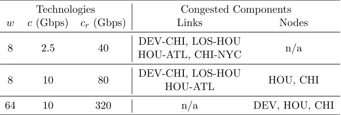
Table 4.1: The bottlenecks of NLR under different technologies

Technologies Congested Components

w c (Gbps) cr (Gbps) Links Nodes

8 2.5 40 DEV-CHI, LOS-HOU n/a

HOU-ATL, CHI-NYC

8 10 80 DEV-CHI, LOS-HOU HOU, CHI

HOU-ATL

64 10 320 n/a DEV, HOU, CHI

topology models rarely take router utilization into consideration.

Also, traffic demands are not uniform across the network. PoPs located at major cities with large population can exchange traffic at a much higher rate than others [35]. There are always some nodes and/or links that carry excessive load, creating bottlenecks. The traffic demands, together with the layout of the physical topology, affect the bottleneck location and intensity. For instance, a “hot spot” NYC in Figure 4.3 is expected to employ mostly direct connections to other PoPs in order to avoid congestion at intermediate nodes, while establishing too many end-to-end lightpaths may exhaust the scarce wavelengths and result in new bottlenecks at the output links. Another big city, Chicago, with five output links will not have such problem though. A realistic virtual topology model thus needs to take into consideration the traffic distribution over physical infrastructure.

Table 4.2: Notations

Notation Definition

Gp = (Vp, Ep) Physical topology with the set of nodesVp and the set of fiber links Ep

Gv = (Vv, Ev) Virtual topology with the set of PoP nodesVv and the set of lightpathsEv

Λ ={λsd} Long-term traffic demand between nodessand d ρL/ρN Maximum lightpath/node utilization

cr Electronic switching capacity at a node c Capacity of each wavelength

w Number of wavelengths per fiber D Average channel length

H Average packet hop distance

T Network throughput

4.2

A Bottleneck-Oriented Design

4.2.1 Problem Definition and Assumptions

Refer to Table 4.2 for the terminology used. Network throughput,T, is the sum of the accom-modated traffic between all node pairs. With an over-provisioned network, T is also known as the maximum scale-up factor of given traffic demands. The WDM virtual topology design problem aims at identifying a virtual topology Ev that maximizes the throughput T, given physical topologyGp, PoP node placement Vv, traffic matrix Λ, and technology constraintsw, c, and cr.

We make the following assumptions: 1) Each physical link is bi-directional and composed of a single fiber supporting w wavelengths. 2) The wavelength-continuity constraint is not considered since a design with no or limited converting capability has been addressed in [52]. 3) The number of transponders at a node matches the number of available wavelengths. Otherwise, it will be a network misconfiguration. 4) Traffic flows go through the smallest possible number of lightpaths, i.e., shortest-path-first (SPF) routing protocol. SPF algorithm may not be optimal for all cases, but it holds well for static network design problems [29].

4.2.2 Key Idea

traffic crossing the router. When routers are the bottlenecks, it is desirable tobypasselectronic processing at routers by creating end-to-end lightpaths. On the other hand, when wavelength capacity is the bottleneck, it is desirable to deploy traffic grooming techniques, thus not by-passing electronic processing, in order to: 1) distribute traffic evenly among parallel lightpaths, and/or 2) spread the load over alternative link paths.

Let ρL denote the maximum lightpath utilization in the network, and ρN denote the maxi-mum node utilization. A virtual topology which mostly relies on end-to-end lightpaths (referred

to as a transparent topology) is thus mostly trying to avoid bottlenecks at routers, and a topology which mostly exploits electronic processing at routers through hop-by-hop lightpaths (referred to as anopaque topology) is trying to avoid bottlenecks at links. An optimal topology design should balance the use of these two schemes to minimizeρ= max{ρL, ρN}.

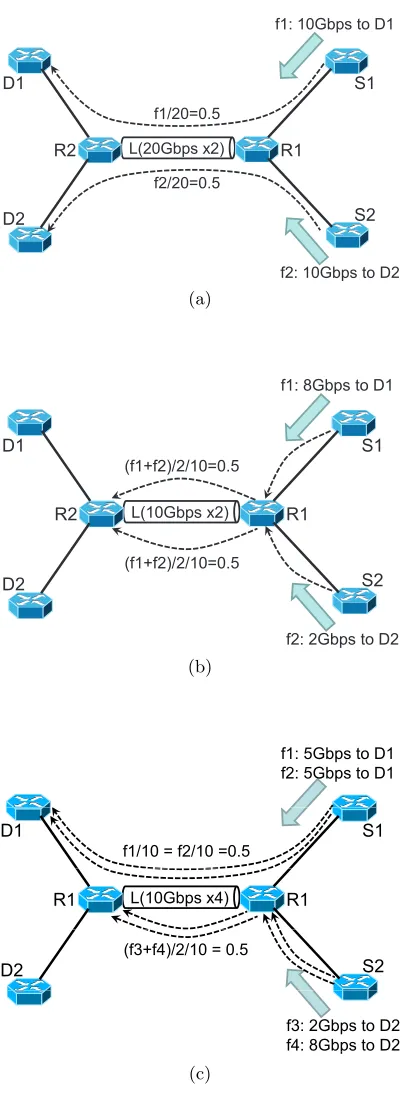
Refer to Figure 4.5 for an example. In this example, two sources S1 and S2 send two flows with rates f1 and f2 towards destinations D1 and D2. The flows cross routers R1 and R2 and the link L connecting them. In Figure 4.5(a), link L has two 20 Gbps wavelengths and the routers, R1 and R2, each has 20 Gbps capacity, i.e., w=2, c=20 and cr=20. If flows f1 and f2 (10 Gbps each in this case) are processed at R1, they will exhaust the router capacity and create node congestion as ρN = (f1 +f2)/20 = 100%. Thus, it is desirable to bypass the routers in Figure 4.5(a) with a utilization ρ = ρL = max{f1/20, f2/20} = 50%. In Figure 4.5 (b), we reduce the wavelength capacity to 10 Gbps (i.e.,w=2, c=10 and cr=20) and let f1 and f2 be 8 Gbps and 2 Gbps, respectively. Bypassing routers in this case leads to ρ = ρL = max{f1/10, f2/10} = 80%, while applying traffic grooming at R1, as shown in

Figure 4.5(b), provides a lower ρ = max{(f1 +f2)/2/10,(f1 +f2)/20} = 50%. Finally, in Figure 4.5(c), end-to-end lightpaths lead to a ρ =ρL _{= 80%, and hop-by-hop lightpaths lead} toρ=ρN = 100%. Neither design is optimal. A layout combining both, as shown in the figure, leads to the bestρ= 50%.

In Table 4.2, the average channel length,D, represents the average number of physical links traversed by a lightpath. The average packet hop distance, H, represents the average number of lightpaths traversed by a traffic flow. Theaverage link hop distance, which is the product of H and D, represents the average number of links traversed by a flow. In following, we derive a lower bound on throughputT in terms ofH and D.

Given the virtual graph Gv and a specific routing scheme, Dand H can be calculated as:

D= w· |Ep|

|Ev|

(4.1)

H= P 1

s,dλsd

X

s,d

λsdX

(ij)

L(20Gbps x2)

S1

S2 D1

D2

f1: 10Gbps to D1

f2: 10Gbps to D2

R1 R2

f1/20=0.5

f2/20=0.5

(a)

L(10Gbps x2)

S1

S2 D1

D2

f1: 8Gbps to D1

f2: 2Gbps to D2 R1

(f1+f2)/2/10=0.5

(f1+f2)/2/10=0.5 R2

(b)

f1: 5Gbps to D1 f2: 5Gbps to D1

S1 D1

f1/10 = f2/10 =0.5

L(10Gbps x4) _R1

R1

S2 D2

(f3+f4)/2/10 = 0.5

f3: 2Gbps to D2

f4: 8Gbps to D2p

(c)

wherepsd_ij = 1 ifλsd employs lightpath (i, j) as an intermediate channel, and psd_ij = 0 otherwise.

|Ep|(or|Ev|) denotes the size of the setEp (orEv). Letλij be the aggregate traffic demand on lightpath (i, j). λij can be expressed as

λij =

X

s,d

λsd·psd_ij (4.3)

Considering the fact that the maximum value is always greater or equal to the average, the lower bounds ofρL _andρN _{are given by:}

ρL≥ 1 |Ev| ·c

X

(ij)

λij =

H·D w·c· |Ep|

X

s,d

λsd (4.4)

ρN ≥ 1 |Vv| ·cr

(X i

X

j λij −

X

s,d

λsd) = H−1

|Vv| ·cr

X

s,d

λsd (4.5)

Since 1/ρL and 1/ρN indicate the maximum scale-up factors on links and nodes, respectively, the throughput T is decided by the one with less value:

T =min{ 1

ρL, 1 ρN} ·

X

s,d

λsd (4.6)

Combining (4.4), (4.5), and (4.6), we end up with

T ≤min{_P|Ev| ·c (ij)λij

,P |Vv| ·cr (ij)λij −Ps,dλsd

} (4.7)

or

T ≤min{w·c· |Ep|

H·D ,

|Vv| ·cr

H−1 } (4.8)

Algorithm 1 The BOA Algorithm

1: INPUT: Virtual topologyGv (a 2-connected graph) 2: repeat

3: Implement SP traffic routing on Gv and compute: 4: T ← the throughput

5: k← the node with maximum utilizationρN

6: (i, j)← the lightpath with maximum utilization ρL 7: if ρN _≥ρL _then

8: S← the list of traffic flows being routed atk 9: whileS 6=∅ do

10: λsd _{← pop the largest flow ofS}

11: try to create a new lightpath (s, d). If fails,do 12: c← connectivity of Gv− {∀(u, v)|psduv= 1}♠ 13: if c >1 then

14: Replace{∀(u, v)|psd_uv= 1} by a channel (s, d) 15: end if

16: end while 17: else

18: tryto add one more parallel (i, j). If fails, do 19: (p, q)←search for the qualified channel♣ 20: if (p, q) existsthen

21: Divide (p, q) into segments containing (i, j) 22: else

23: Divide (i, j) into pt-to-pt channels 24: end if

25: end if

26: Recompute the new scale-up factorT0 27: untilT0 < T

28: OUTPUT: new virtual topologyG0_v (a 2-connected graph)

4.2.3 Algorithmic Details

18). In case the creation of the new parallel channel fails due to the shortage of wavelengths, we search for one existing “longer” channel that can be fragmented into (i, j) and other segments (see lines 19-21). As marked by♣, a qualified channel must traverse all links traversed by (i, j) and we select the one which carries the least traffic load. The initial input Gv can be either a real virtual graph in use, or a baseline configuration such as MMT [41] and MST [19].

The convergence of Algorithm 1 to a lowerT is guaranteed sinceT0< T is checked after each iteration. Furthermore, the algorithm cannot lead to a disconnected graph since we always start with a 2-connectedgraph (line 1) and enforce2-connectivity in each iteration (as marked by♠

in Algorithm 1). 2-connectivity is a common property of core networks to ensure resilience [35]. Each iteration of BOA takesO(|Vv|3lg|Vv|) of time and O(|Vv|2) of space in a worst case. The total number of iterations performed depends on input graph Gv and is bounded by O(|Vv|2).

4.3

Performance Evaluation

Our experiments are based on two real networks: NLR (Figure 4.1) and Sprint (Figure 4.3), and two fictitious networks: NLR-inspired and Sprint-inspired. According to the data from 2006, NLR carries few hundred terabytes of daily traffic on an eight-wavelength OC-96 WDM infrastructure utilizing Cisco CRS-1 routers [7]. We create a NLR-inspired network by adding three extra links into NLR, (SEA-CHI), (LOS-DC), and (HOU-NYC), reflecting NLR’s next-generation backbone infrastructure proposal in 2009. Sprint is a petabyte scale Tier-1 ISP. It uses eight-slot Cisco CRS-1 routers and sixteen-wavelength DWDM fibers, with each wavelength 10 Gbps in capacity [10]. To represent emerging DWDM technologies, we create a Sprint-inspired network which has the number of wavelengths on each link upgraded to 64. The detailed network configurations are summarized in Table 4.3.

Table 4.3: ISP Network Configurations

Network Λ w c cr

(Tbps) (Gbps) (Gbps)

NLR 2 8 5 160

NLR-inspired 2 8 5 160

Sprint 10 16 10 320

Sprint-inspired 50 64 10 320

Since ISP traffic demand is rarely published, we consider two traffic models:

Table 4.4: Network Bottleneck and Design Strategy

Network Traffic Pattern Desired Design Change of Metric ρL (%) ρN (%)

NLR uniform opaque 82→68 46→56

real opaque 68→55 42→50

NLR-inspired uniform opaque 70→62 44→52 real combination 50→44 40→45 Sprint uniform combination 32→27 24→26 real combination 26→22 20→23 Sprint-inspired uniform transparent 28→40 70→45 real transparent 27→40 68→44

Vp =Vv, and all node pairs require the same bandwidth. This scenario ignores intentionally the distinctness of node structure and exhibits a significant degree of traffic uniformity since no hot-spot is present.

ˆ Real-World Traffic: The required bandwidth between two nodes is proportional to the product of their populations (refer to traffic model in Chapter 3), and traffic has to be aggregated at a PoP in the vicinity before being transmitted. This scenario reflects the demand irregularity and hierarchical structure of Internet backbone networks.

Each simulation starts with a simple MMT configuration (see Chapter 2) and then BOA is applied till all traffic demands are accommodated. Depending on the setup, the resulting virtual topology could be transparent, opaque or a combination thereof. The results are listed in Table 4.4. In all cases, BOA balances ρL and ρN thus reduces the bottleneck utilization. Since NLR has initial link congestion much larger than its node congestion (i.e.,ρL_{= 82% and} ρN = 46% for uniform traffic, andρL= 68% andρN = 42% for real-world traffic), the bottlencks are on the links. The resulted NLR virtual graph is laid out with all point-to-point connections. Surprisingly, even with an opaque graph, NLR still suffers from link congestion more than from the nodes (i.e., 68% > 56% for uniform traffic, and 55% > 50% for real-world traffic). This observation suggests that as traffic volume increases, NLR is likely to set up more parallel channels along the congested links to treat the bottleneck. Also, one observes that by adding three extra links, the bottleneck utilization in the NLR-inspired network decreases significantly. Particularly, ρ = ρN = 45% in NLR-inspired network compared to ρ = ρL = 55% in NLR network. The optimized NLR-inspired network has both transparent and opaque layouts.

NLR Sprint Sprint−inspired 0 10 20 30 40 50 60 70 80 90 100

Maximum Lightpath Utilization (%)

MRU MLDA BOA

(a)

NLR Sprint Sprint−inspired

0 10 20 30 40 50 60 70 80 90 100

Maximum Node Utilization (%)

MRU MLDA BOA

(b)

NLR Sprint Sprint−inspired

0 0.5 1 1.5 2 2.5 3 3.5 4 4.5 5

Maximum Scale−up Factor

MRU MLDA BOA

(c)

traffic). The resulting virtual graph has both point-to-point and end-to-end connections and matches well with the published Sprint map. For the Sprint-inspired network, it is obvious that a significant shortage of switching capability at nodes (i.e., ρN _{= 70% for uniform traffic, and} ρN = 68% for real-world traffic) pushes the resulting graph towards a transparent layout. Our results imply that the Sprint network is likely to evolve towards a transparent virtual graph in order to maximize the throughput.

We next compare the performance of BOA to two other popular heuristics MLDA and MRU (the discussions of MLDA and MRU can be found in Chapter 2) in terms of the maximum lightpath utilization, maximum node utilizations, and network throughput. As shown in Figure 4.6, BOA outperforms the other heuristics, leading to better network throughput. It achieves that by balancing the maximum link utilization and the maximum node utilization. These results reinforce our arguments that none of the existing heuristics performs best in all setups. BOA on the other hand can pinpoint the bottleneck elements, which is crucial to maximize the network throughput.

4.4

Summary

Chapter 5

Towards a Robust and Green

Internet Backbone Network

Previous virtual topology design models mainly aim at maximizing the network throughput by spreading out the load evenly among network fabrics. That is reasonable because the throughput is limited by the bottleneck elements, whether at routers or links. Recently, however, energy concerns are highlighted as a sizable fraction of total electricity supply in U.S. was used by network equipment, and a significant part was devoured by Internet backbone infrastructure. A green Internet with as little as 1% lower power can save more than ten billion dollars per year. Most recent design models thus aim at minimizing energy consumption by aggregating traffic along fewer routes while allowing devices on other routes to sleep [25].

Hence, there is an obvious trade-off. On one side, backbone networks are typically over provisioned with bandwidth redundancy. A large part of electricity bill and heat dissipation costs are wasted by under-utilized resources with balanced traffic load. On the other side, Internet traffic is highly fluctuant, containing spikes that ramp up quickly on any links and/or nodes [57]. Concentrating the load on few active routes to save energy may cause the network to become vulnerable to sudden spikes, resulting in severe congestion. A virtual topology design that can handle both network robustness and energy conservation is desirable for backbone networks. Unfortunately, existing design models explore only one factor and not the other.

to energy savings and resource utilization closely matching the optimal solution but only with polynomial time complexity.

The rest of this chapter is organized as follows. In Sections 5.1 and 5.2, we discuss the network power and congestion models. In Sections 5.3 and 5.4, we show the key idea and propose our design model. In Section 5.5, we present the results on two published ISP networks. We finally summarize in Section 5.6.

5.1

Network Architecture and Power Consumption Model

We target a backbone network running IP-over-WDM. As shown in Figure 5.1, a typical back-bone structure consists of nodes interconnected by WDM fiber links. Each node is equipped with bothoptical cross-connect (OXC) andcore router. At WDM-layer, the OXCs switch light-paths transparently from input links to output links, and at IP-layer, core routers route data packets (when converted into electronic domain) over the lightpaths. Associated with a core router are severalaccess routers that aggregate low-rate flows from local areas. Other devices essential to a WDM system are as follows: 1) A pair oftransponders (labeled as T/R), i.e., one transmitter and one receiver, are needed at the endpoints of each lightpath for data transmis-sion and E-O/O-E convertransmis-sions. 2) A pair of optical multiplexer and demultiplexer (labeled as De/Mux) are deployed at fiber ends to multiplex/demultiplex different wavelengths. 3) Erbium-doped fiber amplifiers (EDFAs) are placed at fiber ends performing pre and post amplification, and along a fiber at certain distance intervals. In IP-over-WDM networks, virtual channels can be configured in two different ways: bypass and non-bypass. In the bypass scheme, a lightpath directly connects the source and the destination (e.g., the solid line connecting nodes 1 and 3 in Figure 5.1). Information is delivered end-to-end without in-transit processing. In the non-bypass scheme, traffic undergoes OEO conversions and IP routing at every intermediate nodes (e.g., the dashed line connecting nodes 1 and 3 in Figure 5.1).

An IP-over-WDM network is a complex engineering structure containing different network devices. We next identify the devices that consume power most.1

OXC Core Router T/R T/R Node 1 OXC Core Router T/R T/R Node 2 OXC Core Router T/R T/R Node 3 Fiber Fiber Access Router Access Router

IP layer IP layer

WDM layer WDM layer

Physical layer EDFA

Amplifier Access Router Access Router Access Router Access Router Access Router Access Router Access Router Access Router Access Router D e /M u x W a v e le n g th s D e /M u x W a v e le n g th s

Figure 5.1: Architecture of an IP-over-WDM backbone network.

base system (i.e., chassis plus processor plus switching fabric), and a traffic-dependent term proportional to the amount of traffic passing through. It should be noted that, a router or a line card can be selectively put in standby to conserve energy if it works at lower rate [14]. The standby mode reduces the operation speed and working power to a minimized level to maintain the basic “context information” such as routing tasks. Its power consumption is assumed to be 0.

ˆ Another primary power contributor is the transponder. According to the product data of Alcatel-Lucent WaveStar OLS [6], a pair of transponders of 10 Gbps lightpath consume eL_{= 146 watts when working and e}L_{= 0 if the lightpath carries no traffic (i.e., standby} mode).

Other devices consume minor power. For example, [48] estimates that one 8-watt EDFA is needed for every 80 km of fiber reach. EDFAs have no standby mode, hence a fixed usage for a given network. Each MEMS-based OXC consumes power in the order of 0.45 watt per connec-tion [55], which is negligible compared to core routers. Access routers are also not considered because they are out of our scope as we focus on backbone infrastructure.

In summary, the overall network power usage, E, is expressed as:

E= X

iis a node

eR_i + X

(i,j)is a channel

where eR_i is the router power usage at node i and eL_(i,j) is the power consumed by the channel between nodesiand j.

5.2

Network Robustness to Traffic Spikes

In general, the Internet intra-domain traffic is predictable. It is not difficult for ISPs to estimate the average traffic volume with reasonable accuracy by considering customer subscription, daily peak hours,etc.However, estimating traffic fluctuations is difficult. To this end, representative traffic patterns are extracted based on history data and observed trends. These patterns serve as possible traffic spikes within next time window with granularity as fine as hour-to-hour [65]. If a design model does not incorporate this information, it may cause congestion at network devices, creating bottlenecks that limit a network throughput. We refer to the ability to handle traffic spikes as networkrobustness.

To investigate the robustness, we use the following model. Given traffic matrix T and a virtual topology designf, the utilization of a lightpath is the percentage of wavelength capacity that is used by traffic crossing the lightpath; the utilization of a router is the percentage of router capacity that is used by traffic crossing the router. The maximum lightpath utilization (MLU), denoted byuL(f, T), is the maximum utilization of all lightpaths. Themaximum router utilization (MRU), denoted by uR(f, T), is the maximum utilization of all routers. MLU and MRU were widely used in previous network designs [41, 57, 66].

An optimal design f, which is most robust to traffic T, is the one that minimizes the maximum (lightpath and router) utilization u(f, T). The resulting optimal utilization, u∗(T), is given by

u(f, T) = max{uL(f, T), uR(f, T)} (5.2) u∗(T) = Minimizef u(f, T) (5.3) To compare different designs, theperformance ratio of an arbitraryf is defined as:

p(f, T) = u(f, T)

u∗(T) ≥1 (5.4)

wherep(f, T) measures how farf is from being optimal.

Now, to account for different traffic patterns, we extend the defined metric to a set of traffic matrices X. In particular, a design is based on an optimization minimizing u(f, X) for all X∈X, formally:

u(f,X) = max{u(f, X) | ∀X ∈X} (5.5)

Table 5.1: Notations

Notation Definition

G= (V, E) physical topology with nodesV and links E w number of wavelengths per fiber

cL capacity of a wavelength

cR electronic switching capacity of a node

u= maximum (link and node) utilization, max{uR, uL}

E total network power consumption T ={tsd} traffic matrix for common demand X={X} traffic matrices for possible traffic spikes

Ω ={ωij} number of parallel lightpaths between nodes i,j

Π ={πmnij } πmnij = 1 if lightpath (i, j) employs link (m, n),πmnij = 0 otherwise. Λ ={λsd

ij} fraction of traffic between sand dthat traverses lightpath (i, j)

b

Λ ={bλsd_ij} fraction of traffic between sand dthat traverses lightpath (i, j)

as part of a non-shortest path

b

Ω ={ω_bij} number of working lightpaths of ωij

Note that in (5.5), the aggregation of u(f, X) is based on the worst-case performance. It can also be done, for example, by taking some type of weighted average. The performance ratio of an arbitraryf onX is:

p(f,X) = u(f,X)

u∗_(X) (5.7)

Lowerp(f,X) translates to a more robust design with regard to the whole set X.

5.3

Problem Statement

5.3.1 Terminology

t35

t14

5

4

(t14_,t35_{, t}45_{) /2} t35 t14

(t14_,t35_{, t}45_{) /2} ( , , )

1

3

t24

t25 _t24

2

(a)

5 4 0

0

0 0

0

1 3

0

t24 _t45

t13 _t23 _t35 _t34 ₀

t , t t23_{, t}25

t34_{, t}35

t13_{, t}23_{, t}35_{, t}34

2 0

(b)

Figure 5.2: Two virtual topology designs on a five-node two-wavelength network (a) minimizing the maximum utilization; (b) minimizing the power consumption. Traffic flows that traverse each lightpath/node are exhibited in the figures.

5.3.2 Problem Formulation

While both network robustness and energy conservation are desirable, the optimization aiming at individual objectives can lead to distinctly different designs. Refer to Figure 5.2 for an example. We assume all node pairs require identical 5 Gbps bandwidth, i.e.,∀(s, d), tsd = 5. Let the channel capacity be 20 Gbps and the capacity of each router port be 15 Gbps. Figure 5.2(a) uses purely non-bypass scheme with no lightpath bypassing any intermediate node. Flows are balanced across the network. The resulting lightpath utilization uL= 3₂·_·t₂₀sd = 37%, and router utilization uR = t₁₅sd = 33%. The maximum utilization is thus u = max{uR, uL} = 37%. There are totally ten lightpaths and five router ports in use in Figure 5.2(a). On the other hand, Figure 5.2(b) combines non-bypass and bypass schemes. Flows are aggregated on fewer channels with uL = 4·₂₀tsd = 100%. Node 1 processes 30 Gbps in-transit tafffic while all other nodes are in idle. There are totally four lightpaths and two router ports activated in this case. The maximum utilization of Figure 5.2(b) is much worse than in Figure 5.2(a), while its power consumption is 60% less.

t13_t35 t13_t14

5

4

t13_,t14_,t35_{, t}45 t13,t35

t13_,t14

0

1

3

t24

t25 t24

2

0

(a)

5 4 t

25_{, t}35

t14_{, t}24

0

0 0

0

1 3

t25 _t45

t24 _t45

t13_{, t}45 t25, t45

t24_{, t}45

2 0

(b)

Figure 5.3: Variants of traffic routings in Figure 5.2 with the same virtual graph. (a) a variant of Figure 5.2 (a) minimizing the power consumption, (b) a variant of Figure 5.2 (b) minimizing the maximum utilization.

while traffic spikes have much shorter duration. It is best to focus energy saving on normal operation.

We thus formulate the problem by separating the energy optimization for common traffic demand T and the bounded congestion level for traffic spikesX:

Minimizef on T : E =PieRi +

P

(i,j)eL(i,j)

Subject to: (1)f is a virtual topology design (2)u(f,X)≤100%

(5.8)

Formulation (5.8) is reducible to another NP-hard problem – minimizing the maximum light-path utilization [66] – because testing uL ≤ 100% for all fs has the same rank as finding the minimumuL_{. Solving this problem is numerically intractable for real-sized networks. This} inher-ent complexity leads us to decompose the complete design into two more tractable subproblems: virtual graph layout (VGL) and traffic routing (TR) [41].

5.4

A Two-Phase Heuristic

5.4.1 Key Idea

link channels through electronic traffic grooming. So the optimality of the two factors is uniform when it comes to VGL. Meanwhile, by comparing Figure 5.3 with Figure 5.2, we observe that a distinctly different TR is deployed as we target one factor instead of the other. For example, Figure 5.3(a) concentrates the flows at one of the two parallel lightpaths on each link to save energy. Figure 5.3(b) balances the load among links/nodes to reduce the maximum utilization. The whole idea is summarized in Figure 5.4.

Robustness

Robustness

VGL

TR

spreadthe load

bypassfor router usage &

VGL

TR

the load g

non-bypassfor channel efficiency

Energy Save

Energy Save

Figure 5.4: Design strategies of two factors on solving each subproblem.

5.4.2 Phase I – Virtual Graphs with Bounded Congestion

In phase I, we find out the virtual graphs with bounded worst-case MLU/MRU against traffic spikes given physical network (i.e.,G,cL,cR,w) and traffic matrices,X. The MLU/MRU values are computed by assuming the shortest-path-first (SPF) traffic routing. The SPF algorithm is implemented in major ISP networks [29].

Recalling Equation (5.7), a virtual topology design f is said to have penalty envelope φif the performance ratio of f on Xis no more than φ(φ >= 1) [57], namely:

∀X ∈X, u(f, X)

u∗_(X) ≤φ (5.9)