Twenty-second mathematical and statistical modeling workshop for graduate students

Twentysecond Mathematical and Statistical

Modeling Workshop for Graduate Students

18 – 27 July 2016

North Carolina State University

Raleigh, NC, USA

Organizers:

Pierre Gremaud, Ilse C.F. Ipsen, Ralph C. Smith

Department of Mathematics

North Carolina State University

This report contains a summary of the

Industrial Mathematical and

Sta-tistical Modeling Workshop for Graduate Students

, held in the Department of

Mathematics at North Carolina State University (NCSU) in Raleigh, North

Carolina, 18 – 27 July 2016.

This was the twentysecond such workshop at NCSU. It brought together

39 graduate students from mainly Mathematics and Statistics Departments

at 31 different universities.

The goal of the IMSM workshop is to expose mathematics and statistics

students from around the country to real-world problems from industry and

government laboratories; interdisciplinary research involving mathematical,

statistical and modeling components; as well as experience in a team

ap-proach to problem solving.

Following last year’s success, the IMSM workshop was extended by a

day to accommodate a Bootcamp on

Building Software in Teams

on the

first day (18 July 2016), where the students learnt about shell commands,

version control and Git,

On the morning of the second day (19 July 2016), industrial and

govern-ment scientists presented six research problems. The presentera, together

with specially selected faculty mentors, then guided teams of 6–7 students

and helped them to discover a solution. In contrast to neat, well-posed

academic exercises that are typically found in coursework or textbooks, the

IMSM problems are challenging real world problems that require the

var-ied expertise and fresh insights of the group for their formulation, solution

and interpretation. Each group spent the remaining days of the workshop

investigating their project, and reported their findings in 20-minute public

presentations on the afternoon of the final day (27 July 2016).

The IMSM workshops have been highly successful for the students as

well as the presenters and faculty mentors. Often projects lead to new

re-search results and publications. The projects can also serve as a catalyst for

future collaborations between project presenter and faculty mentor. More

information can be found at

http://www.samsi.info/IMSM16

Sponsors

Statistical and Applied Mathematical Sciences Institute (SAMSI)

Center for Research in Scientific Computation (CRSC)

Department of Mathematics, North Carolina State University

Instructor for Bootcamp on Building Software in Teams

John Pearson (Duke University)

Problem presenters

Jordan Massad (Sandia National Laboratories)

Agustin Calatroni, David Hall, Herman Mitchell and Hoang Tran (Rho Inc.)

Matthew Farthing, Ty Hesser and Bertrand Lemasson (US Army Corps of

Engineers)

Elizabeth Mannshardt and Brett Gantt (EPA), Jessica Matthews (CICS)

Ted Rieger (Pfizer)

Faculty mentors

Alen Alexanderian (North Carolina State University)

H. Thomas Banks (North Carolina State University)

Lea Jenkins (Clemson University)

Kimberly Kaufeld (North Carolina State University)

Emily Lei Kang (University of Cincinnati)

Arvind Saibaba (North Carolina State University)

Ralph Smith (North Carolina State University)

Projects

Uncertainty-enabled thermal stress management of engineered

mul-tilayered structures

Problem presenter:

Jordan Massad

Faculty mentor:

Ralph Smith

Students:

Sameed Ahmed, Johannes Joachim Brust, Cassie Noelle Marker,

Paul Miles, Siamak Rabieniaharatbar, Peter Wills

Finding patterns in protein chip data to probe the immunological

mechanisms of nut allergies

Problem Presenters:

Agustin Calatroni, David Hall, Herman Mitchell,

Hoang Tran

Faculty mentor:

Emily Lei Kang

Students:

Francis Bilson Darku, Shisi He, Md Akhtar Hossain, Sheng Ren,

Hui Fen (Sarah) Tan, Imelda Trejo-Lorenzo

Using remote sensing for bathymetry estimation in coastal

envi-ronments

Problem Presenter:

Ty Hesser

Faculty mentor:

Lea Jenkins

Students:

Lasith Adhikari Charnelle Bland, Lopamudra (Monty) Chakravarty,

Wenbin Dong, Olaniyi Samuel Iyiola, Gail Muldoon, Clint Seinen

Distilling ecological value from hydraulic complexity

Problem presenters:

Bertrand Lemasson, Matthew Farthing

Faculty mentors

Kimberly Kaufeld

Students:

Cong Cao, Jose Cortes, Mingyuan Gao, Elizabeth Heines, Weifan

Liu, Nickalaus Alexander Painter, Karlan Wolfkill

Fusing surface and satellite-derived PM observations to determine

the impact of international transport on coastal PM2.5

concentra-tions in the western U.S.

Problem Presenters:

Elizabeth Mannshardt, Brett Gantt, Jessica Matthews

Faculty mentors:

Alen Alexanderian, Arvind Saibaba

Students:

Neha Dilip Bora, Tuo Chen, Dana Victoria Cochran, Kelly

Dougan, Gautam Sabnis, Chuanping Yu

Quantitative approaches for the examination of physiological

vari-ability in cardiometabolic disease

Problem Presenter:

Ted Rieger

Faculty mentor:

H. Thomas Banks

Students:

Lukas Bystricky, Yuzhou Chen, Glen Wright Colopy, Yifan Cui,

Angelica Gonzalez, Yifei Liu, Rebekah White

Uncertainty-enabled Thermal Stress Management of Engineered Multilayered Structures

Sameed Ahmed1_{, Johannes Brust}2_{, Cassie Marker}3_{, Paul Miles}4_{, Siamak Rabieniaharatbar}5 _{Peter Wills}6 Problem Presenter: Jordan Massad, Robert Kuether7_{; Faculty Mentors: Ralph Smith}8

Abstract

Multilayered structures are of importance for a variety of industrial applications. The temperature at which they are made and used can differ greatly, which can effect the structures’ reliability due to resulting residual stress and deflection. The trial-and-error method often used by experimentalists has improved multilayered structure design, but this approach lacks efficiency in producing desired results. Mathematical modeling, simulation, and computation of multilayered structures provide a way to streamline the process of choosing design parameters for desired results. In this paper, we take an existing model of thermal deformation of multilayered structures and expand it by including temperature dependence of material properties and layer gradation. We demonstrate the efficacy of the model by applying it to three representative structures. We then further analyze multilayered structures both analytically and numerically by studying the models sensitivity, optimization, and uncertainty. We conclude by summarizing our observations and providing design suggestions.

1

Introduction

Multilayered structures are critical for a large number of applications including microelectronics, thermal barrier coatings, and ceramic capacitors. Depending on the application, the multilayers can be a combination of different classes of materials such as, ceramics, metals, polymers, or solders. Materials are combined due to the necessity of achieving certain service conditions of a part. These service conditions vary with location and therefore the material requirements also vary with location. For example, a multilayered high temperature co-fire ceramic is combined with aluminum to form a microelectronic device package with an integral window as shown in a report by Peterson and Watson [4]. More recently, the use of additive manufacturing has allowed for the creation of gradient materials. Carroll et al. [1] investigated the creation of a pure Inconel 625 to pure Stainless Steel 304L graded sample. Zhang et al. [5] investigated the creation of a gradient thermal barrier coating going from ZrO2Y2O3 to NiCrAlY.

An intrinsic difficulty with multilayered structures is that the combination of different materials can cause the formation of residual stresses or deflection. Residual stress is defined as the stress present in the object while in the absence of any external load or force [3], while deflection is the related to the degree of curvature of the material [2]. The introduction of deflection or residual stress is due to the differing mechanical properties and processing parameters of the creation of the materials. When a multilayered material is heated or cooled, the materials in each layer expand and contract differently. If the expansion or contraction is inhibited by the other layers, then residual stress is introduced. If the expansion or contraction of the layers is partially allowed, it causes the material to curve.

A typical method for creating multilayered structures is through trial-and-error. However, the use of modeling, computational tools, and software to predict specific properties can narrow down experimental options, which saves time and money by greatly reducing the need of trial-and-error.

This work presents the formation of a computational tool that allows for the robust design of multilayered structures given certain specifications and outputs the temperature dependent residual stress and deflection. This tool allows for uncertainty quantification and the ability to optimize the residual stress and deflection to specific variables of interest.

1_{Applied Math, University of South Carolina} 2_{Applied Math, University of California Merced}

3_{Materials Science and Engineering, Pennsylvania State University} 4_{Mechanical Engineering, Florida State University}

5_{Math, Purdue University}

6_{Applied Math, University of Colorado} 7_{Sandia National Laboratory}

The structure of this report is as follows. Section 2 formally defines the problem and model used. Section 3 outlines the testing of the model, sensitivity analysis, design optimization and uncertainty quantification. Section 4 summarizes our work and provides suggestions for future capability enhancement.

2

The Problem

To be able to develop a computational tool, we first have to build a forward model that calculates the residual stress and deflection. Second, we also need to be able to minimize the residual stress and deflection and optimize different variables while providing uncertainty quantifications.

2.1

The Forward Model

The first step is to define the design parameters of multilayered structures below:

Tref The temperature where the strain and the stress are zero

Tmin The minimum temperature that the material is subject to

Tmax The maximum temperature the material is subject to

m The gradient exponent

Ei Young’s modulus of each material i (Temperature dependent)

n Number of layers in a gradient layer

N Number of layers

h Total thickness of the multilayered material

zi Thickness of layer i

νi Poisson’s ratio of each layer i (Temperature dependent) (0 <ν < 0.5) εth

i Thermal strain of each layer i (Temperature dependent)

Table 1: The important design variables for multilayered structures.

From these variables we started with Hall’s [2] model by defining the stress in Cartesian coordinates as

εx=εth+ [σx−ν(σy+σz)]/E (1)

εy=εth+ [σy−ν(σx+σz)]/E (2)

εz=εth+ [σz−ν(σx+σy)]/E, (3)

where εx, εy, εz are the strains along the x, y, and z directions, and σj is the stress. We then assume an axisymmetric disk in thex−y plane, which impliesσz= 0 and due to symmetryεx=εy andσx=σy. This leads to the simplification

ε=εth+σ(1−ν)/E (4)

where we remove subscripts to simplify notation. Recall that z is the coordinate corresponding to the thickness of the plate. Assuming the strain is a linear function ofz, the strain can then be written as

ε=εB+ z

h(εT−εB), (5)

whereT andB refer to the top and bottom of the plate, respectively. We consider that for a plate consisting ofilayers, each layer will have its own set of material properties. Therefore the stress within theith_{layer can} be found by combining (4) and (5), yielding the stress at the boundaries:

σi= Ei 1−νi

εB+ z

h(εT −εB)−ε th i

. (6)

N

X

i

Pi= 0, N

X

i

Mi= 0 (7)

wherePi is the radial force per unit perimeter in theithlayer, andMi is the moment per unit perimeter. The force and moment are defined with respect to (6) by

Pi=

Z zi zi−1

σdz= Ei 1−νi

(εB−εthi )(zi−zi−1) +

(εT −εB)(zi2−zi2−1) 2h

(8)

Mi=

Z zi zi−1

zσdz. (9)

After simplification, we find that

εtop= 1 F

h

(C2−D2)[6h(A1−B1)−3(A2−B2)] + (C1−D1)[4(A3−B3)−6h(A2−B2)]

i

(10)

εbottom= 1 F

h

4(A3−B3)(C1−D1)−3(A2−B2)(C2−D2)

i

, (11)

where

F = 4(A1−B1)(A3−B3)−3(A2−B2)2 (12)

Ak= N

X

i ¯

Eizik (13)

Bk= N

X

i ¯

Eizik−1 (14)

Ck= N

X

i ¯ Eiεthi z

k

i (15)

Dk= N

X

i ¯ Eiεthi z

k

i−1. (16)

Here ¯Ei=Ei/(1−νi) is the biaxial modulus andzi is the z-location of the top of theith layer. From these simplified equations the mag stress in the middle of the layers can be calculated:

σmag =

h(σ_i+σ_i−1)2−σ_iσ_i−1

3

i12

(17)

The radius of curvature is found to be

ρ= h εT −εB

, (18)

where ρ is the radius of curvature and h is the thickness of the total multilayered material. From ρ the deflection can be calculated as

2.2

Gradient Layers

In order to deal with gradient layers, we implemented the work by Zhang et al.[5]. Assuming layeristarts with pure material R and is graded to pure material S, the layer is divided into sublayersn. Then uniform properites are assumed for each sublayer by finding theEn,εthn, andνn by

En =ER

z

tn

m

+ES

1−z

tn

m

(20)

νn=νR

z

tn

m

+νS

1−z

tn

m

(21)

εn =εR

z

tn

m

+εS

1−z

tn

m

(22)

At this point the temperature dependence of the thickness and material properties must be determined.

2.3

Temperature Dependence

Since the strip is much thinner in thez-direction than in thex- andy-directions, we have assumed that the thermal deformation of each sub-layer thickness is negligible. However, for certain materials and applications, this thickness deformation needs to be accounted for. We determine the effect of thickness deformation on stress, radius of curvature, and deformation analytically and numerically. Thickness deformation is given by

zi=γizi0, (23)

where zi0 is the thickness of layer i before thermal deformation, zi is the thickness of layer i after thermal deformation, and γi is the factor by which the thickness of layer i deforms. We assume uniform thickness deformation, that is, each sub-layer deforms by the same factor. We then find that

γi=γ, i= 1, ..., N. (24)

Upon inspection of the formulas for top strain, (11), and bottom strain, (12), it can be seen that the numerators and denominators both have thickness to the fourth power. Since the factor for thickness deformation is the same in each sub-layer, this factor can be factored of out each term in the numerator and denominator and canceled. Therefore, top strain and bottom strain are invariant to thickness deformation. The only remaining term in the stress that depends on the thickness deformation is z_h. Again, the thickness deformation factor cancels out here. Therefore, the stress is also invariant to thickness deformation. As seen in (19), the radius of curvature linearly depends on thickness deformation,

ρ=γρ0. (25)

Forρ >0 the deflection is given by

δ=ρ−pρ2_−L2 ₍₂₆₎

= L

2

ρ+pρ2_−L2 (27)

≈ L

2

2ρ (28)

≈ 1

γδ0, (29)

where the second equality is from multiplying by the conjugate and simplifying, and the third approximation is due toL << ρ. Thus the deflection depends on thickness deformation inversely linearly.

H

Figure 1: This a graphical showing of the temperature dependence of multiple materials properties.

with varying thickness. The results match our analytical results. So for this work the temperature dependence of the thickness has found to be negligible and not included.

Up to this point the assumption has been made that the materials properties,Ei,εi, andνiare constant, when in reality these properties vary with temperature as discussed in the table above. An example of the variance of materials properties as a function of temperature is shown below:

To handle the temperature dependence, tables of the variables at discrete temperatures are inputted and a linear interpolation is done to the temperatures of interest for the specific problems. With the forward model in place, testing, sensitivity, optimization and uncertainty were implemented.

3

The Approach

3.1

Forward Model Testing

To test the model three different realistic problems were tested and are presented here.

Figure 2: When m=1 the change between material E0 andEF is linear but when m > 1 then there is more E0 before going toEF and when m < 1 then there is moreEF.

Figure 3: A picture of the set up for problem A.

Case 1 Case 2 Case 3 Case 4

Alumina Alumina Alumina Alumina

z = 1 mm z = 1 mm z = 1 mm z = 1 mm

PbSn solder PbSn solder PbSn solder PbSn solder

z = 0.1 mm z = 0.5 mm z = 0.1 mm z = 0.5 mm

Invar Invar Invar Invar

gradation gradation gradation gradation

Titanium Grade 2 Titanium Grade 2 Titanium Grade 2 Titanium Grade 2

z = 4 mm z = 4 mm z = 4 mm z = 4 mm

n = 50 n = 50 n = 50 n = 50

m = 0.5 m = 0.5 m = 2 m = 2

PbSn solder PbSn solder PbSn solder PbSn solder

z = 0.2 mm z = 1.0 mm z = 0.2 mm z = 1.0 mm

Stainless Steel 316 Stainless Steel 316 Stainless Steel 316 Stainless Steel 316

z = 5 mm z = 5 mm z = 5 mm z = 5 mm

Table 2: The different cases studied for problem A.

Figure 4: Problem A: Displaying the temperature dependence of strain magnitude in the bottom solder layer, stress magnitude in the Alumina and Stainless Steel and deflection.

Figure 5: Problem A: Displaying boundary stress versus thickness for all cases.

Based on Figure 5 it can be seen that the thicker the solder the lower the stress and deflection. It is also seen that with m = 0.25, meaning that there is more TiG2, there is less stress and deflection in the gradient layer. The conclusions from this test show that in order to optimize the stress and deflection increasing the soder thickness and decreasing m is best.

Problem B) looked at a three layered material with aTref= 295 K, aTmax= 400 K and a Tmin= 220 K.

Figure 6: A picture of the set up for problem B.

Aluminum Aluminum Aluminum

z = 0.5 mm z = 0.5 mm z = 0.5 mm

Aluminum Aluminum Aluminum

gradation gradation gradation

Copper Copper Copper

z = 4 mm z = 4 mm z = 4 mm

n = 50 n = 50 n = 50

m = 0.25 m = 1.0 m = 4.0

Copper Copper Copper

z = 2 mm z = 2 mm z = 2 mm

The variation of the gradient exponent m was studied. The m < 1 means the gradient material moved faster to pure Al, a m = 1 means taht it was a linear step from Cu to Al and a m > 1 means it took longer to get to pure Al. The boundary stress versus thickness at T = 220 K, the stress magnitude in each layer i at T = 200 K and the deflection versus temperature were plotted to compare the different m values.

Figure 7: Problem B: Displaying the temperature dependence of deflection, the magnitude stress in the Al layer, the magnitude of stress in the Cu layer and the boundary stress versus thickness at two temperatures.

Based on Figure 7 it can be seen that m > 1, meaning having more Cu, leads to a lower deflection but has a larger boundary and magnitude stress. The case when m < 1, meaning more Al, has the lowest deflection but still the second highest boundary and magnitude stress. Finally, when m = 1 we have the lowest stress and the second lowest deflection. In this case if you are trying to optimize to stress and deflection m = 1 would be best but this is very application dependent.

Figure 8: Depiction of the setup for problem C.

We imagine a setup

Npairs =



      

      

Material1 Material2 Material1 Material2

.. .

Figure 9: Problem C: Displaying the effect of changing the number of layers.

From Figure 9 it is seen that increasing the number of layers decreased the deflection and stress. At some point the results begin to converge even with the increae in layers. The minimum deflection solution was largly independent of thickness ratio. Based on our above results, a more thorough sensitivity testing of the effects of each variable on the output was performed.

3.2

Sensitivity

To begin the sensitivity testing, we first tried an analtyical study. We considered every parameter with respect to temperature. But based on the complexity of the equations we decided to look at two cases instead.

3.2.1 Analytical Sensitvity Testing

In what follows, we consider different cases to demonstrate the difficulties of Analytical sensitivity analysis. So we first consider the general case and try to break down to simpler cases but at the end analytical analysis is very demanding.

For the general case we take the derivative of σi with respect to temprature T. Using ˚1 and ˚2 we get the following first order differential equation with respect to the temperature which can be solved by the integration factor method to obtain:

f(T)∂σi

where

f(T) = F_¯ Ei

(31)

g(T) = (F 0

¯ Ei

−FE¯

0 i ¯ E2 i ) (32)

h(T) = [4(A3−B3)0(C1−D1) + 4(A3−B3)(C1−D1)0−3(A2−B2)(C2−D2)0−3(A2−B2)0(C2−D2)]+ 6z[(A1−B1)0(C2−D2) + (A1−B1)(C2−D2)0−(A2−B2)0(C1−D1)−(A2−B2)(C1−D1)0]−(F th)0. Thererfore we obtain:

∂σi ∂T σi

= h(T)

σi −g(T)

f(T) . (33)

Now we consider the case where ¯Ei is independent of change inT, i.e ∂

¯

Ei

∂T = 0. Then we have

∂Ak

∂T = 0 =

∂Bk ∂T , ∂Ck ∂T = N X i=1 ¯ Eithi

0

z_ik, ∂Dk ∂T =

N

X

i=1 ¯ Eithi

0

z_ik₋₁, ∂F

∂T = 0, g(T) = 0. (34)

which yields

f(T)∂σi ∂T =

4(A3−B3)(C1−D1)0−3(A2−B2)(C2−D2)0]−F thi 0

+ 6z[(A1−B1)(C2−D2)0−(A2−B2)(C1−D1)0

. ∂σi ∂T σi =

4(A3−B3)(C1−D1)0−3(A2−B2)(C2−D2)0]−F thi 0

+ 6z[(A1−B1)(C2−D2)0−(A2−B2)(C1−D1)0

[4(A3−B3)(C1−D1)−3(A2−B2)(C2−D2)]−F thi + 6z[(A1−B1)(C2−D2)−(A2−B2)(C1−D1)]

Lastly we take the derivative w.r.t the thermal strainth. Due to the fact ∂

¯

Ei ∂th j

= 0 we obtain

∂Ak ∂th j

= 0 = ∂Bk ∂th j

, ∂Ck ∂th j = N X i=1 ¯

Eizkiδij = ¯Ejzjk, ∂Dk ∂th j = N X i=1 ¯

Eizki−1δij= ¯Ejzjk−1, ∂F ∂th

j

= 0, g(T) = 0.

Then we have

F ¯ Ei ∂σi ∂th j =

4(A3−B3)(C1−D1)0th−3(A2−B2)(C2−D2)0th]−F ∂th

i ∂th

j

+6z[(A1−B1)(C2−D2)0th−(A2−B2)(C1−D1)0th

=E¯j[4(A3−B3)(zj−zj−1)−3(A2−B2)(z2j−z

2

j−1)]−F ∂th

i ∂th

j

+ 6z[(A1−B1)(zj2−z

2

j−1)−(A2−B2)(zj−zj−1)

∂σi ∂th j σi = ¯

Ej[4(A3−B3)(zj−zj−1)−3(A2−B2)(zj2−zj2−1)]−F

∂th_i ∂th j

+ 6z[(A1−B1)(zj2−zj2−1)−(A2−B2)(zj−zj−1)] [4(A3−B3)(C1−D1)−3(A2−B2)(C2−D2)]−F thi + 6z[(A1−B1)(C2−D2)−(A2−B2)(C1−D1)]

3.2.2 Sensitivity Analysis For Problem A

We test the sensitivity of certain quantities to certain parameters in problem A. The quantities of interest (QOI) are the stress in alumina, the strain in solder 1, the strain in solder 2, and the defection. The varied parameters are the thickness of solder 1, the thickness of solder 2, the exponent of gradation, the Young’s modulus of stainless steel, the Poisson’s ratio of stainless steel, and the thermal strain of stainless steel. These are listed in Table 4. Each parameter is varied while the others are kept fixed. The reference value for the varying parameter and the value of the fixed parameters are those given in Problem A. Except for the exponent of gradation, all parameters are varied within 50%. The exponent of gradation is varied within a factor of five. The QOI are then calculated for each parameter value.

Quantities of Interest Varied Parameters

σN δ zs1 E1

εs1 zs2 ν1

εs2 m εth1

Table 4: List of quantities of interest and varied parameters for sensitivity analysis in Problem A.

Figure 16: Sensitivity plots. They-axis is the percent change in the QOI, and thex-axis is the percent change in the varied parameters.

Figures 10 - 15 show the individual results of (QOI) versus (parameter value), whereas Figure 16 shows the collective results in a sensitivity plot of (percent change in QOI) versus (percent change in parameter). These results show that a QOI can be very sensitive to a certain parameter and not others. For instance, strain in solder 1 and deflection vary much more rapidly with respect to thermal strain of stainless steel than with other parameters. These results also show that which parameter has the greatest effect depends on the QOI. Strain in solder 2 is most sensitive to gradation exponent, while the other QOI are most sensitive to thermal strain of stainless steel. Another observation is that certain QOI respond nonlinearly to changes in parameters. Most notably, stress in alumina varies nonlinearly between a 40% and 10% reduction in thermal strain of stainless steel. Such analysis can help streamline experimental design for desired effects.

3.2.3 Sensitivity Analysis For Problem B

In this section we do the sensitivity analysis for problem B. We compute the L2 _{norm and deflection while} changing the following parameters in the Copper:

• Exponent of Gradation m

• Young’s ModulusE

• Thermal Strainth

• Thickness of graded layers between Aluminum and Copper

Case 1) Sensitivity analysis of Exponent: The exponent varied in the interval of [m₅,5m].

Figure 17: Sensitivity plots of the gradient exponent m.

The sensitivity analysis in Figure 17 shows that varying the exponent m leads to a nonlinear behaviour of

L2 _{norm of Aluminum and Copper, and deflection. TheL}2 _{norm of Aluminum reaches a minimum around}

Figure 18: Sensitivity plots of the Young’s modulus.

The sensitivity analysis shown in Figure 18 that as the Young’s ModulusE increases for Copper and theL2 norm of Aluminum increses. However the deflection shows an almost linear behaviour.

Figure 19: Sensitivity plots of the Poisson’s Ratio.

As it can be seen in the Figure 19 theL2_{norm increses as the Possion’s Ratioν increases. The sensitivity} analysis ofν is done with the constraint of 0 <ν < 0.5 is satisfied. For deflection we see similar behaviour as the case for Young’s Modulus.

Figure 20: Sensitivity plots of the thermal strain.

From Figure 20 the sensitivity analysis shows linear decrease in the L2 _{norm of Aluminum as the thermal} strain increases.

Figure 21: Sensitivity plots of the gradient thickness.

Figure 21 shows the the L2 _{norm of Aluminum and Copper decrease nonlinearly as the graded thickness}

increses.

3.3

Optimization

Seeing how the sensitivity of a parameter is greatly dependent on the quantity of interest and the may not be linear we looked at how we could optimize these parameters based on the originial problems.

3.3.1 Optimization of Problem A

For our optimization, we started by focusing on the Problem A) decribed in the forward model subsection. We explore two distinct objective functions; stress in the insulating alumina layer, and total deflection. In application, we would likely apply some linear combination of these, but for illustrative purposes we will examine them separately.

We calculate the stress (and deflection) over a range of temperatures. We then have a two variable function σ(z, T) (in the case of stress) as per (6), from which we must compute a scalar “norm”. In our case, we take the maximum in space and anL1 average in temperature to obtain this

kσk ≡

Z Tf Ti

max z∈Al2O3

σ(z, T)dT. (36)

Computationally, the integral is approximated by a first-order discretization method. We allow the two thicknesses to range between 0.05 and 1 mm.

1) Varying Solder Thickness

We first examine an optimization scenario based on the first scenario described above, but allow the thickness of the solder to vary.

Figure 22: Solder thickness versus temperature-averaged maximum stress in alumina layer. The optimal value is highlighted, and occurs at approximately (.59, 1).

This optimum is calculated using MATLAB’sfminconfunction. The well-behaved nature of the objective surface (shown in Figure 22) allowsfminconto run quickly and without complication using its default settings. When we employ deflection as our objective (temperature averaged similar to (36)) we find that the minimum deflection occurs on the boundary of our optimization region, that is to say when both solders have the maximum thickness of 1 mm. This is unsurprising, since increased thickness would intuitively decrease the deflection. The objective function plotted against solder thickness (not shown) is approximately planar, and increases with decreasing thickness.

Since the objective surfaces are straightforward, one can readily guess the behavior if we are to use a linear combination of the two surfaces. To wit, the optimal value for the first solder layer (alumina to Ti/invar) is between 0.59 and 1 (depending on the coefficients of the linear combination in our objective function), and the optimal value of the second solder layer remains 1 mm.

2) Varying Exponent of Gradation

Now we will examine the effect of varying the exponent of gradation on our various objective functions. That is to say, we will fix the solder thicknesses at 1 mm and allow the exponentm to vary.

Proceeding as before, we first examine a temperature-averaged maximum stress in the alumina. We allow

the exponent of gradation to range between m = 0.1 andm = 10. Figure 23 shows a plot of max average

stress against gradation exponent. The optimal value is clearly visible, and is calcualted to be approximately

m= 0.76.

Figure 23: Average max stress against exponent of gradation. Minimum occurs atm≈0.76.

In the situation where we wish to minimize deformation, we do not obtain an interior minimum. The endpoingm= 10 yields minimal deformation, as seen in Figure 24. This indicates that the optimal choice for minimizing deflection is to make the material entirely titanium, as we might expect.

Figure 24: Average deformation against exponent of gradation for a disk of radius of 100 mm. Minimum occurs at right endpoint, wherem= 10 and “graded” material is almost entirely titanium.

3) Varying Materials in Top and Bottom Layers

Alumina Silicon Carbide Silicon Nitride

Stainless Steel 23.41 62.91 93.97

Aluminum 91.22 59.71 59.96

Alloy 42 48.08 81.47 106.44

Kovar 34.65 71.62 102.51

Nickel Ni-200 24.25 66.99 98.42

Figure 25: Temperature-averaged max stress in insulating layer for different materials, measures in megapascals (MPa). Temperatures range from 300K to 450K.

Alumina Silicon Carbide Silicon Nitride

Stainless Steel 0.46 0.55 0.61

Aluminum 0.88 0.98 1.06

Alloy 42 0.16 0.07 0.01

Kovar 0.05 0.04 0.10

Nickel Ni-200 0.37 0.45 0.51

Figure 26: Temperature-averaged deformation for different materials, measures in millimeters (mm). Temper-atures range from 300K to 450K. Disk radius is 100 mm.

These results in table 25 and 26 show that your quantity of interest is very important in reading the results. For example, if you are interestec in the lowest deformation you would pick Alloy 42 and Silicon Nitride. However, if you are interested in the lowest max stress in the insulating layer you would choose Alumina and Nickel. Based on these results if you were trying to minimize both stress and deformation the best choice would be Alumina and Kovar.

3.3.2 Optimizing the thermal strain

After investigating the optimization of Problem A we began investigating how to optimize thermal strain. For the remainder of the subsection we investigate conditions that lead to the equality

εT =εB. (37)

First let

ABk ≡Ak−Bk= N

X

i=1

Ei0 zik−zik−1

CDj ≡Cj−Dj = N

X

i=1 εth,iE

0 i

zj_i −zj_i−1, so that

εT = 1

F (CD2(6hAB1−3AB2) +CD1(4AB3−6hAB2)) εB =

1

F (4AB3CD1−3AB2CD2), withF = 4AB3AB1−3 (AB2)

2

. Now we obtain for the condition (37) that

εT −εB = 6h

CD2 CD1

= AB2

AB1 .

In the remainder the unknowns are E_i0, εth,i and the thicknesses zi−zi−1 = hi. Observe that CD2 =

PN

i=1εth,iE 0

ihi(zi+zi−1) and that AB2=P

N i=1E

0

ihi(zi+zi−1) so that

PN

i=1εth,iE 0

ihi(zi+zi−1)

PN

i=1εth,iE 0 ihi

=

PN

i=1E 0

ihi(zi+zi−1)

PN

i=1E 0 ihi

= 0. (38)

From 38 we may conclude that equality will hold whenever

εth,i=c, for alli.

That is the thermal strain coefficient is the same for all materials included. Therefore we conclude that if the goal is to design a material that is robust under temperature changes, then it is advisable to select materials that have similar thermal strain properties. To verify this analytical result we construct a hypothetical structure that is equal to the structure from problem a), with the exception that we let the thermal strains in the middle layer be the sameεth

2 =εth3 =εth4 =cand the ones in the remaining layers satisfyεth1 =εth5 =F·c. Here 0≤F ≤1 is a fraction that measures how close the thermal strains are to each other. We find that the minimum for|εT −εB|is precisely found whenF = 1 or when all the strains are equal to each other:

Figure 27: We vary the scalar F which measures how close the thermal strains for a 5 layered material are. At the point whenF = 1 all materials have equalεth

i and|εT −εB|is minimized.

3.3.3 Optimizaiton of Problem C

Our objective is to minimize the total structure deflection. Let the deflection be denoted byδ(h1, h2, N;, T) = δ(h;N, T) in which h= [h1, h2]T,N vary andhis fixed for all temperatures. In particular we discretize the temperature as

Tj=T0+j

T1−T0

J =T0+j∆T, 0≤j≤J;

whereT1, T0denote the final and initial temperatures (Kelvin), respectively. Mathematically our optimization problem is

minimize h∈R2,N∈Z+

q(h, N;T), subject to: N hT1

=h,

where the objective function,q, is defined as

q(h, N;T) = ∆T T1−T0

M

X

j=1

0 < h, and J is a fixed integer. This formulation of the problem requires optimization over continuous (h) and an integer variable (N). Because the computation of the objective function is cheap, and the solution of mixed variables optimization problems is in general very hard, we decide to break down the problem into separate optimization problems for a specified number of layers. That is, we setup a grid of layers

Ni =i, where∈ {1,2,· · · },

which allows us to fix the integer variableN so that we obtain an objective functions that only depend on the continuous variableh. We thus optimize M separate problems, for which theith _{problem is of the form}

minimize h∈R2

q(h;T, Ni), subject to: Ni hT1

=h,

fori= 1,2,· · ·. In a particular scenario we seth= 300mmand the materials as

Material1≡Al2O3, Material2≡Al. Moreover we set

T0 (Lower temperature) = 298K, T1 (Upper temperature) = 800K, Tref (Reference temperature) = 600K, J (# Temperature intervals) = 100,

h(Structure height) = 300mm, L(Half-length of structure) = 300mm,

Our initial guess for the thicknesses (mm) is scaled by the number of pairs

hi=

1

i[ 100 200 ] T_.

Figure 28: Plot of the objective function with a representation of the constraint for a different number of layers. As the number of layers increases the magnitude of the objective function decreases, although the general form of the objective does not change significantly.

For this problem we observe that the deflection of the material decreases as the number of pairs is increased. In particular we find that one setup may be slightly superior to the other ones. As a guide for designing a particular structure we display the ratio of the thicknesses that correspond to a solution of the optimization problem h∗2

Figure 29: A plot of the objective function as the number of pairs in the structure is varied. It appears that a structure ofN= 28 pairs has an objective value that is lower than its neighboring setups.

From Figure 28 and 29 it was seen that as the number of layers increases the magnitude of the objective function decreases, although the general form of the objective does not change significantly. It also appears that a structure ofN = 28 pairs has an objective value that is lower than its neighboring setups. Solutions are found where the materials are equally thick or the second material is twice as thick as the first one.

3.4

Uncertainty

When analyzing a model, it is important to remember that any uncertainty in input parameters leads to uncertainty in the output. The uncertainty in the input is typically caused by random sources such as noise within measuring devices or subtle variation from one test specimen to another. Ideally, these influences are as controlled as much as possible to decrease the amount of uncertainty in the input. In the real world this can never be accomplished, but we can set reasonable bounds on the expected value for each input, often including some factor of safety. It then becomes important to observe and quantify how large of effect this input variation will have on the output.

example of the randomness of input variables is shown in Figure 30 on the left and a corresponding distribution of an output quantity of interest is shown in Figure 30 on the right.

Figure 30: Uncertainty of input parameters (a) leads to uncertainty in output (b). Note the uncertainty from input to output is not necessarily a linear relationship.

One important observation to point out is that the distribution of output parameters will not necessarily match the distribution of the input parameters. In the cases reported below, we have assumed a uniform distribution about nominal parameter values. Upon evaluating the output based on a random sampling from these uniform distributions, the quantities of interest clearly do not have uniform distributions (see Figure 30). In other words the mapping from input to output is nonlinear.

The other observation to be made when considering uncertainty quantification is the deviation in the output. Refinement of input parameters may lead to reduced uncertainty in the output, but it may be at the expense of the design criteria. In other words, a given input may lead to a higher mean magnitude of stress, but with less deviation. This provides confidence that the results will be in the predicted range, which is often more important that simply reducing the magnitude of a certain quantity as much as possible.

The next question to be answered is how many samples to take? Pure random sampling is acceptable, but potentially cost prohibitive. An alternative approach is demonstrated in the Section 3.4.1.

3.4.1 Latin Hypercube Sampling

When employing Monte Carlo techniques, it is important to optimally sample the parameter space. Simply running pure random samples many times will lead to a converge density of the output as the number of samples go to infinity. How many samples are actually required is dependent on the problem, and potentially prohibited by cost. Alternatively, one can sample the input parameter space using the Latin Hypercube sampling method.

The basic premise of Latin Hypercube sampling is to optimally observe all combinations of defined input spaces. Picture a two-dimensional grid sampling space, where each cell corresponds to a sample position. If the points sampled from this space satisfy the requirement that no two points are in either the same row or column, then this is what is called a Latin square. Latin Hypercube is the multidimensional analogue to the square.

Given a set ofP input variables that will be sampledN times, the corresponding number of combinations for a Latin Hypercube is

NP−1. (39)

seen in Table 5 the mean and variance of the deflection for Case Study B at the lowest temperature (220 K) converges to a stable distribution as the number of samples increases. However, by using Latin Hypercube sampling the stable distribution is reached with orders of magnitude less samples.

Random Latin Hypercube

log10(N) µ σ2 log10(N) µ σ2

2 -0.467 0.791 2 -0.463 0.786

3 -0.465 0.788 3 -0.463 0.786

4 -0.464 0.787 4 -

-5 -0.464 0.786 5 -

-Table 5: Mean and variance of deflection from Case Study B at T = 220 K. Using Latin Hypercube sampling converges to a stable output distribution much faster than a random technique. The mean values are reported in [mm] and the variance in [mm2].

3.4.2 Uncertainty Problem A

For Problem A, we consider the effect of uncertainty in multiple input parameters. The material properties of Alumina, Stainless Steel, solder, and both ends of the graded layers are considered uncertain. In addition the thickness of each layer is assumed to have uncertainty and even the exponent of gradation. This leads to an input parameter space with 23 random variables. Each of these random inputs were assumed to have uniform variation, but as seen in Figure 31 the output uncertainty is not necessarily uniformly distributed.

(a) Stainless Steel,T = 220 K (b) Alumina,T = 220 K

(c) Stainless Steel,T = 220 K (d) Alumina,T = 220 K

(a) Deflection,T = 220 K (b) Deflection, T = 220 K

Figure 32: Problem A - Tref = 456 K: Deflection of structure (a) Normalized Histogram and (b) Estimated CDF.

3.4.3 Uncertainty Problem B

(a) Copper, T = 220 K (b) Alumina, T = 220 K

(a) Copper, T = 220 K (b) Alumina, T = 220 K

(c) Copper, T = 400 K (d) Alumina, T = 400 K

(c) Copper, T = 400 K (d) Alumina, T = 400 K

(a) Deflection,T = 220 K (b) Deflection, T = 400 K

(c) Deflection,T = 220 K (d) Deflection, T = 400 K

Figure 35: Problem B -Tref = 295 K: Deflection of structure (a,b) Normalized Histogram and (c,d) Estimated CDF. (a,c). Note absolute value of deflection is report to ease the interpretation of the cumulative distribution plots.

As seen in Figures 33-35 the maximum magnitude of stress is very different depending on the operating temperature. Case 3 and 4 appear to reduce stress the most at the lowest temperature; however, at the highest operating temperature Case 3 results in a larger magnitude of stress in both the bottom and top layer. Depending on the criteria it may be important to have a design that produces similar results over the entire operating regime. Under those conditions Case 4 would be advantageous for reducing the stress because it works over a broader temperature range.

As opposed to problem A, the deflection is not necessarily minimized in the same way as the stress. The deflection is smallest for Case 3 at both the low and high temperatures as seen in Figure 35. If reducing the deflection in the structure is more important than reducing the stress, than Case 3 may be the best design choice. This highlights the complexity noted previously that the design choice is affected by many factors.

4

Summary and Recommendations

dependence. We then tested the model on three representative multilayered structures. Based on these prob-lems we then looked at the sensitivity, optimization, and uncertainity quantificiation of the input variables and processing parameters.

Based on the testing we saw that the optimal design depends much on what are the application and design criteria. Optimizing one criterion may be detrimental to another. The way a particular structure should be made leads to different strategies and therefore different optimizations. Sensitivity analysis highlights that the change in quantities of interests with respect to the change of different parameters has a nonlinear trend. Also certain parameters have more impact on particular quantity than others. Therefore depending on the application and cost, the quantity of interests deteremine which parameters can be studied to achieve optimal output. From uncertainity analysis we observed how changes to the nominal design can result in improved reliability probablisitcally. Finally we estimated that material gradation can significantly improve multilayered structure performance. Therefore, we suggest continued development of advanced manufacturing techniques.

5

Appendix

Figure 36: Diagram of the multilayer structure. On the left is the structure before thermal deformation. On the right is the structure after thermal deformation, with the circle completing the curve drawn in.

Figure 36 shows a multilayer structure of disk radius R and thicknessh. The diagram on the left is the structure before thermal deformation. The diagram on the right is the structure after thermal deformation, with the circle completing the curve drawn in. We assume that the deformation is so small that the horizontal line segment from the end of the structure to the center remainsR. The radius of curvature, deflection, angle of curvature, arc length of the bottom of the structure, and arc length of the top of the structure areρ,δ,θ, R1, andR2, respectively. The bottom and top strains are given by

εB := ∆R1

R = ρθ−R

R (40)

εT := ∆R2

R =

(ρ+h)θ−R

R , (41)

where the arc length formula is used for the second equality. Subtracting the bottom strain from the top strain and rearranging yields

θ= R

h(εT−εB). (42)

Since

sinθ= R

we have

R ρ = sin

_R

h(εT −εB)

, (44)

from which we get the radius of curvature in terms of known quantities,

ρ= R

sin R_h(εT −εB)

. (45)

Since the deformation, and thus the deflection, are so small, we can assume that the angle of deflection is also very small. This allows the approximation

sinθ≈θ. (46)

Using this approximation in (42) and (43) and rearranging yields a simpler, but accurate, formula for the radius of curvature in terms of known quantities,

ρ= h εT −εB

. (47)

From Figure 36, we obtain

(ρ−δ)2+R2=ρ2, (48)

from which we get the deflection in terms of known quantities,

δ=ρ−pρ2_−R2_{. (49)}

References

[1] B.E. Carroll et al. “Functionally graded material of 304L stainless steel and inconel 625 fabricated by directed energy deposition: Characterization and thermodynamic modeling”. In: Acta Materialia 108 (2016), pp. 46–54.issn: 13596454.doi:10.1016/j.actamat.2016.02.019.

[2] Peter M Hall. “Thermal expansivity and thermal stress in multilayered structures”. In: Thermal stress and strain in microelectronics packaging. Springer, 1993, pp. 78–94.

[3] Claude A Klein and Richard P Miller. “Strains and stresses in multilayered elastic structures: The case of chemically vapor-deposited ZnS/ZnSe laminates”. In:Journal of Applied Physics 87.5 (2000), pp. 2265– 2272.issn: 0021-8979.

[4] Kenneth A Peterson and Robert D Watson.Bi-level microelectronic device package with an integral win-dow. Jan. 2004.

Finding Patterns in Protein Chip Data to Probe the Immunological Mechanisms

of Nut Allergies

Francis Bilson Darku1, Shisi He2, Md Akhtar Hossain3, Sheng Ren4, Hui Fen Tan5, Imelda Trejo-Lorenzo6

Mentors: Emily Lei Kang4_{, David Hall}7_{, Agustin Calatroni}7_{, Hoang Tran}7

Abstract

Peptide microarrays are an important tool used to investigate various biological reactions, such as the interactions between the immune system and food allergens. However, peptide microarray data is very noisy and human labeling of bad spots is time-consuming and costly. In this paper, we utilize an approach from machine learning,PositiveUnlabeled learning, to predict bad spots when only some bad spots, and no good spots, have been labeled. Our contribution is two-fold: firstly, we demonstrate the use of a distance metric induced by the random forest to identify points dissimilar to known bad spots, and then perform supervised learning to discriminate between known bad spots and predicted good spots. Secondly, we perform extensive feature engineering to create novel features that fully utilize the design of the microarray. Our results with leave-one-out cross validation show that PU learning is able to predict bad spots given only labeled bad spots with 96% accuracy. The addition of engineered features further improves prediction accuracy by 2%. However, a caveat with these results is that this prediction accuracy is for one microarray with many labeled bad points. Future work involves generalizing the model to prevent the model from overfitting to one microarray.

1

Introduction

Allergies are caused by the immune system reacting to common harmless substances, like pollen, as if they were pathogenic. These reactions trigger a cascade of physiological responses that may be mild in some individuals and life threatening in others. Resent publications have been showing that food allergies are rising worldwide and is more remarkable in the infant population [1, 2]. In the United State, food allergies affects nearly 5% of adults and 8% of children. Among children age 0 to 17 years, the prevalence of food allergies increased from 3.4% in 1997-1999 to 5.1% in 2009-2011. A cross-sectional study of infants from a single clinic in China over a 10-year period estimated an increase in food allergy from 3.5% to 7.7%. Furthermore, recent studies focusing on peanut allergy indicated increases, with a doubling in the United Kingdom or tripling the United States, in diagnoses over the past 10 years [1].

The international growing prevalence of food allergy has captured the attention of the scientific community and government agencies. They have focused on the study of improving detection, diagnosis and therapeutics treatment for this specific type of allergy [3]. It has been identified that eggs, milk, peanuts, tree nuts, soy, wheat, crustacean shellfish, and fish are the most common food allergens. Peanut and nuts are the most common foods associated with severe allergic reactions (25.2%), followed by milk (21.1%), and shellfish (17.2%) [4]. Medications, such as antihistamines and corticosteroids, can be used to reduce symptoms and can be life-saving during acute episodes. However, there is no current treatment for food allergy. There is evidence that the interactions between the immune system and specific sequence of food proteins called peptide will help to develop immunotherapy treatments [2, 5].

Analyzing protein microarray data, which are obtained from images of a microchip with proteins spotted onto a surface, is a useful and most promising method for tracking and analyse the reaction between the immune system and allergic peptides [20]. However, the sophisticated and sensitive method of obtaining microarray data introduces different defects in the data which consequently makes the data analysis very

1_{Department of Statistics, University of Texas at Dallas}

2_{Department of Biostatistics, Bioinformatics and Biomathematics, Georgetown University} 3_{Department of Epidemiology and Biostatistics, University of South Carolina}

4_{Department of Mathematical Sciences, University of Cincinnati} 5_{Department of Statistics, Cornell University}

complex and even after taking enough precautions, the analyses may conclude misleading interpretations. Having a good algorithm to detect the defective array data can be a very important development towards feeding a clean and reliable dataset to the analysis techniques in next phases. This further can lead to more efficient and reliable conclusions. This research focuses on finding a learning algorithm to detect the defective data points in protein microarrays.

2

Problem Statement

A protein microarray data is gathered through steps of very sophisticated and sensitive experimental procedure, as mentioned before. To put it in simple words, in such an experiment, the proteins are arrayed onto a solid glass slide. The probe molecules, antibodies, are then added to the array. Any reaction between the probe and the protein emits a fluorescent signal. A microarray scanner is used to acquire the fluorescent signal data at two different wavelengths, 635 nm and 532 nm. Each individual location of protein-probe on the array is known as a spot. The scanner assigns a circular spot indicator to each spot. A collection of spot indicators is called a block. There can be several blocks on a single array, depending upon the type and configuration of the arrayer used to place the spots on the slide. Figure 1 shows how a microarray image looks like.

Figure 1: A microarray image. Image adapted from Larese et al. [6]

Despite the richness of information obtainable from a microarray, it reasonably may has high variability due to bad or defective spots. Spot can be defective because of different factors arising from manufacturing process such as nonspecific hybridization, batch effects or array defects, as well as for biological reasons. It is very important to filter out the bad quality spots at early steps in microarray analysis to avoid noisy data and consequent misleading conclusions [6]. Figure 2 exhibits some examples of good and bad spots that a microarray may contain.

Microarray analysis tools such as Spot and GenePix Pro allow a human expert to manually flag out bad spots within a protein microarry. However, this is a tedious and error-prone procedure given the large number of available spots. Therefore, it is need to have a computer algorithm that can detect defective microarray spots by using different characteristics or measures of spots. Such an algorithm can speed up the bad spot detection process as well as can ensure a reliable data set for further analyses.

3

Exploratory Data Analysis

3.1

Data description

The protein microarray data employed in this research were obtained from a group of tree nut and peanut allergic sufferers sampled from multiple cohorts and clinical trials in Europe and the United States. The technical procedure of obtaining the data involved using GenePix Pro, a prominent microarray image analysis software in current times. Data was provided by Rho Inc8_{. The data comprised of ten microarrays, each of}

them represents an individual.

Figure 2: Examples of good (a) and bad spots (b) - (g). Image adapted from Larese et al. [6]

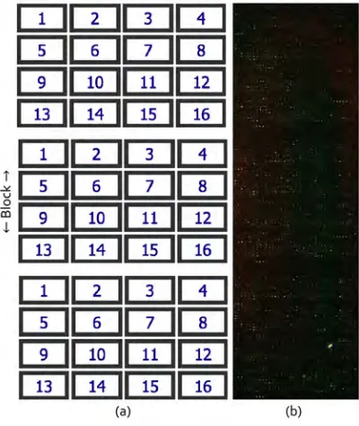
One microarray has 3 chips, and each chip has 1,760 spots - making a total of 5280 spots on an array. Spots in a microarray are arranged in 3 chips, each chip has 16 blocks while there is a 11×10 arrangement of 110 spots in each block. Figure 3 shows a side-by-side view of design skeleton and actual image of the microarray.

Figure 3: (a) The array design skeleton and (b) Actual array image from GenePix Pro.

Once a microarray chip is scanned, GenePix Pro generates different statistical data including various ratios of the fluorescence intensity at two different wavelengths. A row in the dataset represents a peptide while a column represents a characteristic of the peptide. The columns in the dataset labeled Name, ID, and Index

help to identify the spots, while there are other measures providing spacial information about the spots on the array. The spatial information gives an insight into the experiment protocol. The remaining columns, variables, in the dataset provide statistical information about the measurement of biological signals from the spots. The biological signals are measurement at two different wavelength, namely - F635 for red andF532

3.2

Descriptive statistics

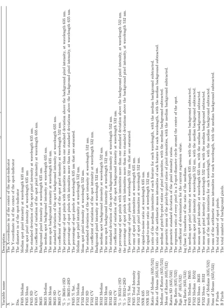
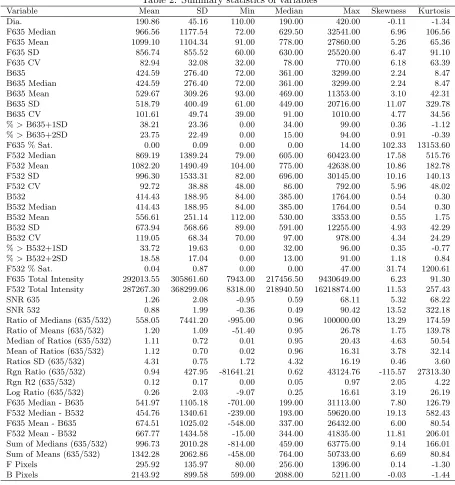
As a very first step of approaching to the data, we computed summary statistics of the different spot features in dataset. Table 2 shows the computed summary statistics.

Table 2: Summary statistics of variables

Variable Mean SD Min Median Max Skewness Kurtosis

Dia. 190.86 45.16 110.00 190.00 420.00 -0.11 -1.34

F635 Median 966.56 1177.54 72.00 629.50 32541.00 6.96 106.56

F635 Mean 1099.10 1104.34 91.00 778.00 27860.00 5.26 65.36

F635 SD 856.74 855.52 60.00 630.00 25520.00 6.47 91.10

F635 CV 82.94 32.08 32.00 78.00 770.00 6.18 63.39

B635 424.59 276.40 72.00 361.00 3299.00 2.24 8.47

B635 Median 424.59 276.40 72.00 361.00 3299.00 2.24 8.47

B635 Mean 529.67 309.26 93.00 469.00 11353.00 3.10 42.31

B635 SD 518.79 400.49 61.00 449.00 20716.00 11.07 329.78

B635 CV 101.61 49.74 39.00 91.00 1010.00 4.77 34.56

%>B635+1SD 38.21 23.36 0.00 34.00 99.00 0.36 -1.12

%>B635+2SD 23.75 22.49 0.00 15.00 94.00 0.91 -0.39

F635 % Sat. 0.00 0.09 0.00 0.00 14.00 102.33 13153.60

F532 Median 869.19 1389.24 79.00 605.00 60423.00 17.58 515.76

F532 Mean 1082.20 1490.49 104.00 775.00 42638.00 10.86 182.78

F532 SD 996.30 1533.31 82.00 696.00 30145.00 10.16 140.13

F532 CV 92.72 38.88 48.00 86.00 792.00 5.96 48.02

B532 414.43 188.95 84.00 385.00 1764.00 0.54 0.30

B532 Median 414.43 188.95 84.00 385.00 1764.00 0.54 0.30

B532 Mean 556.61 251.14 112.00 530.00 3353.00 0.55 1.75

B532 SD 673.94 568.66 89.00 591.00 12255.00 4.93 42.29

B532 CV 119.05 68.34 70.00 97.00 978.00 4.34 24.29

%>B532+1SD 33.72 19.63 0.00 32.00 96.00 0.35 -0.77

%>B532+2SD 18.58 17.04 0.00 13.00 91.00 1.18 0.84

F532 % Sat. 0.04 0.87 0.00 0.00 47.00 31.74 1200.61

F635 Total Intensity 292013.55 305861.60 7943.00 217456.50 9430649.00 6.23 91.30

F532 Total Intensity 287267.30 368299.06 8318.00 218940.50 16218874.00 11.53 257.43

SNR 635 1.26 2.08 -0.95 0.59 68.11 5.32 68.22

SNR 532 0.88 1.99 -0.36 0.49 90.42 13.52 322.18

Ratio of Medians (635/532) 558.05 7441.20 -995.00 0.96 100000.00 13.29 174.59

Ratio of Means (635/532) 1.20 1.09 -51.40 0.95 26.78 1.75 139.78

Median of Ratios (635/532) 1.11 0.72 0.01 0.95 20.43 4.63 50.54

Mean of Ratios (635/532) 1.12 0.70 0.02 0.96 16.31 3.78 32.14

Ratios SD (635/532) 4.31 0.75 1.72 4.32 16.19 0.46 3.60

Rgn Ratio (635/532) 0.94 427.95 -81641.21 0.62 43124.76 -115.57 27313.30

Rgn R2 (635/532) 0.12 0.17 0.00 0.05 0.97 2.05 4.22

Log Ratio (635/532) 0.26 2.03 -9.07 0.25 16.61 3.19 26.19

F635 Median - B635 541.97 1105.18 -701.00 199.00 31113.00 7.80 126.79

F532 Median - B532 454.76 1340.61 -239.00 193.00 59620.00 19.13 582.43

F635 Mean - B635 674.51 1025.02 -548.00 337.00 26432.00 6.00 80.54

F532 Mean - B532 667.77 1434.58 -15.00 344.00 41835.00 11.81 206.01

Sum of Medians (635/532) 996.73 2010.28 -814.00 459.00 63775.00 9.14 166.01

Sum of Means (635/532) 1342.28 2062.86 -458.00 764.00 50733.00 6.69 80.84

F Pixels 295.92 135.97 80.00 256.00 1396.00 0.14 -1.30

B Pixels 2143.92 899.58 599.00 2088.00 5211.00 -0.03 -1.44

Within the dataset, some observations have been flagged 0(unknown if a good or a bad spot) by default,

Table 3: Distribution of flagged spots across arrays

Array Flag

No Name -100 -75 0

(Bad) (Empty) (Unknown)

1 AB44PA 1 1155 4124

2 AE125PA 11 1146 4123

3 AS151PS 18 1146 4116

4 AW37PA 18 1155 4107

5 HW142PS 7 1146 4127

6 JBN108PA 136 1146 3998

7 JCG117PA 11 1146 4123

8 JTH106PA 9 1146 4125

9 MT 0 1146 4134

10 PS 3 1155 4122

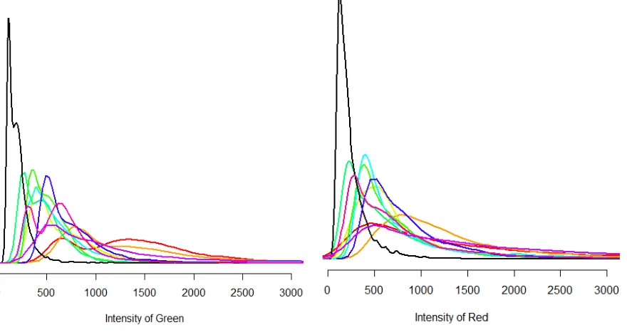
To investigate the possible sources of variation in intensities of spots, the distribution of the median in-tensities for red and green signals were plotted for each array. The plot in the left of Figure 5 is the densities of the green signals while the plot on the right is the densities for the red signals. It can be seen that the distribution of the signal intensities varies from array to array for under the two colors. These differences could be due to technical issues or biological differences that may exist in between the individuals from whom the blood samples were taken.

Figure 5: Left: Densities of median green signal intensities per array. Right: Densities of median red signal intensities per arrays

3.3

Data visualisation

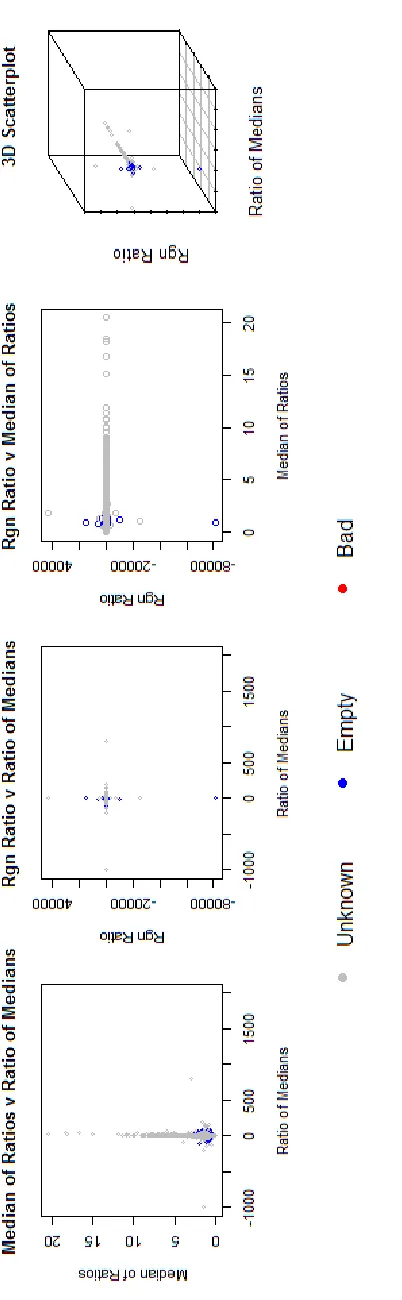
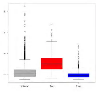
Figure 7: Boxplots of some variables by flag.

3.3.3 Heatmaps and array

Using the data obtained from GenePix Pro, images of the array were reconstructed using theF532 Medianfor green signals andF635 Medianfor red. These images with help of their respective heatmaps provided a visual images of the GenePix outputs. Thus, high and low signals, as well as systematic errors, could be visually inspected.

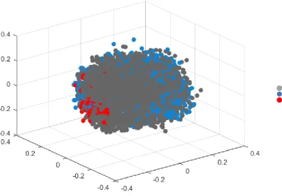
3.3.4 Principal component analysis

Due to the high dimension, many variables, of each observation, visualising each observation while taking into account all variables is almost impossible without employing some kind of dimension reduction techniques. Principal component analysis was performed on the data to project the observation into 2 and 3 dimensions. The first two principal components accounted for 46% of the variation in the data while including the third principal component increased it to 58%. In order to account for about 80% of the variation in the dataset, the first seven principal components have to be used which, in other words, does not help in dimension reduction. Figure 9 shows plots of the first three principal components.

Figure 8: From the left, regenerated output of GenePix Pro for spot intensities under wavelength F532 and F635 respectively, followed by their respective heatmaps.

Unkown Empty Bad

3.3.5 Multidimensional scaling

Multidimensional scaling was performed on the dataset set for array 6. The results for scaling the data into two and three dimensions can be found in Figure 10. The figure does not show any grouping and no distinct features can be seen.

Unkown Empty Bad

Figure 10: Multidimensional scaling.

3.4

Variable selection

Now, we want to have a smaller number of variables to describe the microarray data. In the output of GenePix Pro, many summary statistics are given. Some variables are directly calculated by others, which means they are highly related. For example,B 635means the background pixel intensity at wave length 635. However, it is exactly the same value of B 635 Median. We want to use statistical methods to automatically detect those variables and exclude them. The other reason to do variable selection is to avoid multicollinearity. Correlation is calculated between each variable to have a brief understanding of data.

The Correlation plot shows the correlation of each variable from GenePix Pro. We can find that many of them are highly correlated. Here are the relationship between some of them:

Coefficient Variance = Standard Deviation

Mean (1)

Mean = Total Protein

Spot Pixels (2)