Copyright 0 1988 by the Genetics Society of America
Design and Analysis of Experiments on Random Drift and Inbreeding
Depression
Michael Lynch
Department of Ecology, Ethology, and Evolution, University of Illinois, Champaign, Illinois 61820
Manuscript received November 16, 1987 Revised copy accepted July 7, 1988
ABSTRACT
While the genetic consequences of inbreeding and small population size are of fundamental importance in many areas of biology, empirical research on these phenomena has proceeded in the absence of a well-developed statistical methodology. The usual approach is to compare observed means and variances with the expectations of Wright’s neutral, additive genetic model for quantitative characters. If the observations deviate from the expectations more than can be accounted for by sampling variance of the parameter estimates, the null hypothesis is routinely rejected in favor of alternatives invoking evolutionary forces such as selection or nonadditive gene action. This is a biased procedure because it treats sequential samples from the same populations as independent, and because it ignores the fact that the expectations of the neutral additive genetic model will rarely be realized when only a finite number of lines are studied. Even when genes are perfectly additive and neutral, the variation among the properties of founder populations, the random development of linkage disequilibrium within lines, and the variance in inbreeding between lines reduce the likelihood that Wright’s expectations will be realized in any particular set of lines. Under most experimental designs, these sources of variation are much too large to be ignored. Formulas are presented for the variance- covariance structure of the realized within- and between-line variance under the neutral additive genetic model. These results are then used to develop statistical tests for detecting the operation of selection and/or inbreeding depression in small populations. A number of recommendations are made for the optimal design of experiments on drift and inbreeding, and a method is suggested for the correction of data for general environmental effects. In general, it appears that we can best understand the response of populations to inbreeding and finite population size by studying a very large number
(>loo)
of self-fertilizing or full-sib mated lines in parallel with one or more stable control populations.T
HE genetic consequences of inbreeding and small population size a r e of importance in many areas of biology. Population bottlenecks, through their in- fluence on random genetic drift within loci and link- age disequilibrium between loci, are thought to play a major role in the speciation process (MAYR 1963;TEMPLETON 1980; but see BARTON and CHARLES-
WORTH 1984). The deleterious consequences of in-
breeding are believed to be involved in the evolution of the mating systems of many plants and animals
(CHARLESWORTH and CHARLESWORTH 1987). In-
breeding depression is also a serious concern in selec- tive breeding programs (FALCONER 198l), in the maintenance of endangered species
C SOUL^
1986), and in the protection of human welfare (CAVALLI-SFORZA and BODMER 197 1). Finally, the genetic stability of control lines is a n implicit assumption in many exper- iments in population genetics (HILL 1972a-d), and uniformity of genetic stock is a n essential requirement for many areas of biomedical research (FESTING 1979).T h e r e is therefore a need for a statistical theory for the analysis of the dynamics of quantitative characters in finite populations. T h e expectations are already
Genetics 120: 791-807 (November, 1988)
well-understood for the case of additive gene action (WRIGHT 1951). Under these circumstances, and in the absence of selection, the expected within- and between-population genetic variances, u&,(O)( 1
-
F ) and 2u&,(O)F, are proportional to the genetic variation in the base population, u&,(O), and to the expected degree of inbreeding, F . Although the within-popu- lation variance declines to zero and the betweenpo- pulation variance builds up to 2u&,(O), the expected mean phenotype over all populations remains stable in time.ROBERTSON (1 952) showed that the situation is more complicated with dominance. T h e presence of rare recessive alleles can cause a n initial inflation of the genetic variation within populations and can alter the rate of divergence of population means. The
limiting values of the within- and between-population genetic variances d u e t o variation in the base popula- tion are the same as in the case of additivity, but there is a n overall change in the mean genotypic value
caused by inbreeding depression. Similar complica- tions arise if there are epistatic interactions between loci (HILL 1982; GOODNIGHT 1987).
792 M. Lynch
been given to the expected dynamics of neutral quan- titative characters, studies on the variation around the expectations are relatively rare (BULMER 1976, 1980; AVERY and HILL 1977, 1979; WEIR, AVERY and HILL
1980; COCKERHAM and WEIR 1983; LYNCH and HILL
1986). T h e theory developed in these papers is essen- tial for evaluating the consistency of observational data with expected patterns, but has had remarkably little influence on the design and analysis of empirical studies. Observed increases in the genetic variance within inbred populations are generally attributed to the dominance effect described by ROBERTSON (RAS-
MUSON 1952; BRYANT, MCCOMMAS and COMBS 1986)
although such changes are also possible with additive genes in populations with linked loci and/or variable pedigree structure. Many published studies on in- breeding depression exist in which there was inade- quate or no control and no attention given to the nonindependence of sequential samples or the impor- tance of genetic drift.
In this paper, methods are developed that allow tests of the null hypothesis that observed genetic changes in small populations are consistent with a neutral additive gene system. T h e general approach will be to assume that L independent replicate lines, each with expected effective size Ne, are isolated from a base population with additive genetic variance uh(0).
T h e mean phenotypes, and the additive genetic vari- ance within and between lines, are then monitored over t = 0,K generations. These have expected values of jig(t), Z&(t), and
gi(t)
respectively, but when only a finite number of lines is observed, the realized valuesp ( t ) , u&(t), and u i ( t ) will vary around the expectations from experiment to experiment. Due to imperfections in the estimation procedure, the observations i ( t ) , Vgw(t), and V i ( t ) will also deviate from the true realized values somewhat. T h e main focus here is on variation in the realization of the process of random genetic drift rather than on the variance of parameter esti- mates caused by sampling error on the part of the investigator. T h e first source of variation (realization variance) is a function of population genetic structure and, for a fixed system of mating, is largely beyond the control of the investigator, while the second (sam- pling variance) can at least be minimized by the use of large sample sizes. Expressions for the sampling variance of population parameters are readily avail- able in textbooks of quantitative genetics, and the two sources of error can be treated as independent and additive. T o simplify the presentation, a balanced experimental design will be assumed throughout.
CORRECTING FOR ENVIRONMENTAL TRENDS
A potential source of error in the analysis of unse- lected lines is the presence of general environmental effects that cause the genotypic mean and/or variance
to shift between generations. Even in the most care- fully designed laboratory experiments, there are many uncontrolled sources of variation, including uncon- scious shifts in the behavior of the investigator, and these may obscure the genetic interpretation of phe- notypic observations in many different ways. For ex- ample, a directional environmental trend that influ- ences all individuals in the same manner can lead to the erroneous conclusion that directional selection or inbreeding depression is operating. If genotype X
environment interaction is present, the mean pheno- types of different lines will vary in response to general environmental effects, and in extreme situations, the direction of response may differ between lines. Fi- nally, if the sensitivity to environmental effects in- creases with inbreeding (LERNER 1954; FALCONER
198 l), genotype X environment interaction can in- flate the apparent rate of divergence of mean pheno- types.
While many empirical studies on random drift and inbreeding lack controls, those that have employed them often suggest parallel trends between controls and experimental lines. WRIGHT’S (1 977) inbreeding experiments with guinea pigs are especially dramatic in this respect. Clear evidence for the development of genotype X environment interaction with inbreeding has arisen in experiments with corn (OBILANA and HALLAUER 1974; BARTUAL and HALLAUER 1976) and with Tribolium (BRAY, BELL and KING 1962). Thus, the need for controls and a technique for utilizing the information they provide is very real.
In the case of selection experiments, the usual ap- proach to removing general environmental effects has been to subtract the mean of a contemporaneous control from the mean of the selected population. An implicit assumption of this treatment is that both the control and selected populations respond in the same manner to general environmental effects; i.e., there is no genotype
x
environment interaction. Moreover, as HILL (1972b) has pointed out, this procedure ac- tually can obscure the genetic response of the selected population if the control mean is subject to substantial sampling error. An alternative approach, suggested by MUIR (1 986a, b), is to treat the control line($ as a covariate. This has the advantage of allowing for genotype X environment interaction of an arbitrary level.Analysis of Drift and Inbreeding 793
signal of the general environmental effect, i.e., explain a maximum amount of the variance of the mean phenotypes of the experimental line. Since highly inbred lines sometimes have enhanced environmental sensitivity, they might fulfill this criterion provided their response to the environment is highly correlated with that of the experimental lines (MUIR 1986b).
Let the observed mean of experimental line i in generation t be
Z(t,i)
= fig(0)+
Q ( t , i )+
eg(t,i)+
e,(t,i) (1)where Q ( t , i ) = the cumulative change in the mean genotypic value up to generation t , and eg(t,i) and
e,(t,i) refer to deviations of the observed phenotypic mean from [iig(0)
+
Ag(t,i)] caused by general and special environmental effects, the latter including measurement error. For the control line, the mean genotypic value is assumed to remain constant during the experiment, so thatZ ( t , c ) = Z(C)
+
eg(t,c)+
e,(t,c) (2)where i ( c ) is the mean phenotype of the control av- eraged over the entire experiment. If the control is replicated, then the elements of this equation refer to averages over all replicates.
Since the general environmental effects are the only correlated components of the control and experimen- tal line means, a partial regression of i(t,i) on i ( t , c ) provides a way of factoring out the general environ- mental effects,
; ( t i ) = a(i)
+
b’(i)Z(t,c)+
d(i)t+
e(t,i). (3)Because of the sampling error of the control means, b’(i) provides a slightly biased estimate of the param- eter
p(i)
= u[eg(i),eg(c)/a2[eg(c)]. An unbiased estimator iswhere a2[e,(c)] is the sampling variance of the control mean within generations, u2[t,eg(c)] is the squared co- variance of i ( t , c ) and t , and u‘[eg(c)] is the variance of control means between generations in excess of the sampling variance. This improved estimator may be employed by substituting the observed variance and covariance components. T h e corrected line means are then estimated by
Z*(t,i) =
Z(t,i)
-
b(i)[Z(t,c)-
Z(c)]. (5)d ( i ) in Equation 3 is an estimate of the rate of evolution of the corrected mean phenotypes.
As a consequence of inbreeding and drift, the rela- tive response of an experimental line to general envi- ronmental effects may change throughout the course of an experiment, in which case the correction factor
would need to be a function of time. T h e occurrence of such change could be examined with the model
Z(t,i)
=a(i)
+
[ b ’ ( i )+
g(i)t]Z(t,c)+
d(i)t+
e(t,i), (6) g ( i ) providing an estimate of the development of gen- otype x environment interaction with time. T h e use of several genetically unique controls will increase the information on general environmental effects for ex- perimental lines and can be implemented by the ad- dition of the appropriate terms to the prevoius for- mulas. Whatever the approach, it is important to realize that each experimental line may develop its own unique response to general environmental effects and should be corrected independently of all other lines.As an example of the application of the technique outlined above, the results of an inbreeding experi- ment with Drosophila melanogaster will be considered. Starting from a large base population, KIDWELL and
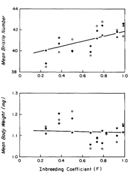
KIDWELL (1966) extracted 20 lines and maintained each by single full-sib matings through 20 generations. T h e base population was also maintained throughout the experiment, and the progeny of four single pair matings from it served as a control for each genera- tion. An undisclosed number of individuals were as- sayed for abdominal bristle number and body weight at irregular intervals. There is a general upward trend in bristle number in both the control and experimen- tal lines throughout the experiment, and the dynamics of mean body weight are also roughly concordant between groups (Figure 1). Based on this visual com- parison, the authors concluded that the lines were strongly influenced by general environmental effects but not by inbreeding depression.
794 M. Lynch
44
0
0 . t
0
0 0
38 I I I I I I
0 0.2 0.4 0.6 0.8 I .o
0 0.2 0.4 0.6 0.8 I .o
Inbreeding Coefficient ( F 1
FIGURE 1.-Observed phenotypic means in inbred (closed cir- cles) and control (open circles) lines of D. melanogaster, and cor- rected values for the inbred lines (stars) obtained by use of Equation 5. The partial regressions are represented by the solid lines. Data are from KIDWELL and KIDWELL ( 1 966).
the temporal variance of mean body weight in the experimental lines was accounted for by variation in the controls.
In addition to their influence on mean phenotypes, general environmental effects may also cause spu- rious, temporal fluctuations in the components of variance. In principle, the procedures outlined above can be extended to the correction of variance com- ponents. However, since the sampling error of vari- ances tends to be very large, reliable corrections of this sort will require large sample sizes.
At least in the case of plants, there may be a way of avoiding all of the above statistical procedures. Pro- vided they are kept cool and dry, seeds can usually be stored for many years. This allows one to grow mem- bers of all generations in a randomized design simul- taneously (RUSSELL, SPRAGUE and PENNY 1963; HAL-
LAUER and SEARS 1973; CORNELIUS and DUDLEY
1974). Even in this case, however, special precautions need to be taken to ensure that phenotypic expression is not influenced significantly by the duration of seed storage or by properties of the seed that may be conditioned by general environmental effects experi- enced by the maternal plant.
DIVERGENCE OF MEAN PHENOTYPES
As outlined in the introduction, a simple prediction of population genetic theory is that the divergence of
mean genotypic values among populations is propor- tional to the degree of inbreeding within populations. This result is expected only for neutral quantitative traits with a purely additive genetic basis, and even then, it begins to break down with the accumulation
of new mutations (CHAKRABORTY and NEI 1982;
LYNCH and HILL 1986). There are more subtle as- sumptions embedded in the theory as well, including the condition that the mode of gene action remains stable with a change in genetic background. Even in the ideal case, the realized between-line variance will
be distributed around the expectation 2a&(O)F(t). Therefore, in order to evaluate the consistency of observations with the neutral, additive gene theory, a statistical description of the between-line variance is required.
T h e usual protocol in genetic drift experiments is to maintain several independent lines under the same experimental conditions and with the same mating system. Let each line be initiated simultaneously with Nm males and N f females randomly extracted from the same base population. Each generation and within each line, N , males are mated randomly to Nf/Nm females, and n offspring are measured from each full- sib family. T h e phenotype of the kth offspring of the mating between male i and female j may be repre- sented as
where gmi and 0, are the additive genetic values of the parents, ( A g , , , i k
+
Ag3k)/2 is the deviation of the off- spring from the midparent additive genetic value caused by segregation, c, is the common environmen- tal effect of female j , and egk is the special environ- mental effect. (Common environmental effects above those caused by maternal environment occur some- times, but here they are assumed to be unimportant.) Because of sampling error of the founder pheno- types, the initial variance of line mean phenotypes has the expectationZi'(0) = ZL(0)
+
a:+
6,'N m
+
Nf
'Analysis of Drift and Inbreeding 795
expected variance of mean phenotypes for t 2 1 is
Z ( t ) = [3j(O)
+
23&(O)F(t)]T h e first term in this formula, which represents the true dispersion of line means, is cumulative over gen- erations, while the remaining terms refer to the vari- ance due solely to finite sample size within lines. Because of the genetic continuity of populations in time, there is an expected covariance between the mean phenotypes in the same line in subsequent gen- erations,
G;(O,t) = Gi(0) for t
>
0, (10)3i(t,t') = Gj(0)
+
23,(O)F(t)for 1
<
t<
t ' . (11)It can be seen from the preceding formulas that the contribution of the segregational and special environ- mental effects variance to the variance of mean phe- notypes is inversely proportional to the total sample size (nlvf), whereas the contribution of common envi- ronmental effects is inversely proportional to the num- ber of full-sib families (Nf). In genetic experiments, it is desirable to remove these sources of variation in order to obtain an estimate of the variance of mean genotypic values unbiased by sampling error. Nor- mally, this can be accomplished by manipulating the mean squares of a nested analysis of variance. T h e within- and between-family components of variance can be isolated from the genetic variance between lines by letting V i ( t ) = [MSI;,,,
-
MSfam(line#nNf be the estimate of a i ( t ) . A slight problem arises if the lines consist of single families, as in the case of selfing and full-sib mating, since the common environmental ef- fects variance cannot be partitioned from the variance of genotypic means. This problem can be eliminated by temporarily expanding each line into S families prior to analysis and substituting S for Nf in the expression for V i ( t ) (LYNCH 1984).Since the number of lines, L , employed in experi- ments is usually rather small, it is of practical impor- tance to have expressions for the sampling variances and covariances of the realized variances of line means. Starting from the same base population, sup- pose that an infinite number of divergence experi- ments, identical in all respects except the realization of the drift process, could be run. At time t , each experiment will have developed a level of between- line genetic variance, &t). Variation will arise among the u$(t) because of variation in the within-population genetic variance among the founder populations, var- iance in inbreeding that develops among the lines, and the observation of a finite number of lines. More-
over, since the line means are a function of their past history, the between-line variances for any particular experiment will be correlated in time. With finite sample sizes, it is also necessary to account for the genetic and environmental variance within and be- tween families and the covariance between the cu- mulative drift variance and the segregation variance.
Expressions for the variance and covariance of be- tween-line variance can be obtained by assuming that measurements have been taken on a scale on which the genetic and environmental effects are normally and independently distributed. In that case, the ex- pected variance of a variance component is twice the expected variance squared divided by the sample size minus one, and approximate expectations for u"[aT(t)]
and u[u?(t), u?(t')] can be obtained by Taylor expan-
sion (APPENDIX).
Equations A1-A3 have been written so that the variance and covariance due to finite sample size are described by the terms within the large brackets. For
t 2 1, these terms decline to zero as the sample size within lines (nNf) increases. T h e earlier terms in the formulas describe the variance and covariance of the true between-line genetic variance, and for a given effective population size, can be reduced only by increasing the number of lines. Thus, ignoring the variance of inbreeding, the squared coefficient of variation of u i ( t ) can be seen to be on the order of
2/
( L-
l ) , and depending on the variation in inbreeding and environmental effects, it can be considerably greater. This implies that studies of phenotypic diver- gence need to be very large to be statistically reliable. For example, if it is desirable to reduce the standard error of the between-line variance to 10% of the expectation, approximately 200 lines would need to be sampled (400 and 300 in the case of selfing and full-sib lines).Of additional concern is the variation among esti- mates of
Gi(t)
caused by variation in inbreeding (WEIR, AVERY and HILL 1980; COCKERHAM and WEIR 1983).Under most mating schemes, some individuals mate by chance with closer relatives than do others. This results in variation in F among members of the same population, and because of sampling, accumulates as between-population variance in average inbreeding. Variance in inbreeding is of special interest because it cannot usually be estimated from empirical data. De- tailed pedigree records may be possible under some experimental protocols, but uncertainties regarding paternity are common. Moreover, the linkage rela- tionships of constituent loci, which influence u2 F , are unknown for virtually all quantitative characters.
Ignoring the variance among founder means, the squared coefficient of variation of &t) is {2[1
+
( N ,796 M. Lynch
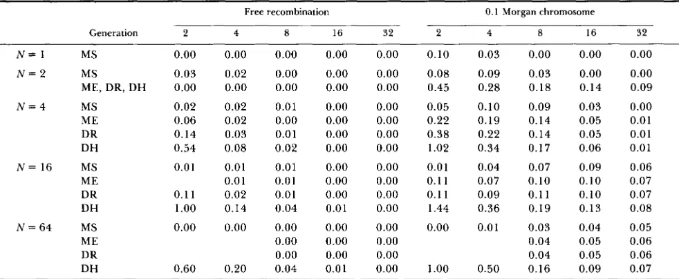
TABLE 1
Values of the squared coefficient of variation of mean line inbreeding, a$(t)/F*(t)
Free recombination 0.1 Morgan chromosome
Generation 2 4 8 16 32 2 4 8 16 32
N = 1 MS 0.00 0.00 0.00 0.00 0.00 0.10 0.03 0.00 0.00 0.00
N = 2 MS 0.03 0.02 0.00 0.00 0.00 0.08 0.09 0.03 0.00 0.00
ME, DR, DH 0.00 0.00 0.00 0.00 0.00 0.45 0.28 0.18 0.14 0.09
N = 4 MS 0.02 0.02 0.01 0.00 0.00 0.05 0.10 0.09 0.03 0.00
ME 0.06 0.02 0.00 0.00 0.00 0.22 0.19 0.14 0.05 0.01
DR 0.14 0.03 0.01 0.00 0.00 0.38 0.22 0.14 0.05 0.01
DH 0.54 0.08 0.02 0.00 0.00 1.02 0.34 0.17 0.06 0.01
N = 16 MS 0.01 0.01 0.01 0.00 0.00 0.01 0.04 0.07 0.09 0.06
ME 0.01 0.01 0.00 0.00 0.11 0.07 0.10 0.10 0.07
DR 0.11 0.02 0.01 0.00 0.00 0.11 0.09 0.11 0.10 0.07
DH 1.00 0.14 0.04 0.01 0.00 1.44 0.36 0.19 0.13 0.08
N = 6 4 MS 0.00 0.00 0.00 0.00 0.00 0.00 0.01 0.03 0.04 0.05
ME 0.00 0.00 0.00 0.04 0.05 0.06
DR 0.00 0.00 0.00 0.04 0.05 0.06
DH 0.60 0.20 0.04 0.01 0.00 1.00 0.50 0.16 0.09 0.07
~
Obtained from data in Table 111 of WEIR, AVERY and HILL (1980). Mating is random in all four mating schemes: MS = ideal monoecious
population including random selfing, ME = monoecy with selfing excluded, DR = dioecy with each offspring produced by a random pairing
of male and female gametes, sex ratio assumed to be 1: 1, DH = monogamous, dioecious population. In the case of a 0.1 Morgan chromosome,
the loci are assumed to be randomly distributed. Slight errors due to rounding may be present. Values under MS were obtained by use of
Equation 27 Of WEIR and COCKERHAM (1 969).
or more. Since the variance in inbreeding is a function of several high-order identity-by-descent measures
(WEIR and COCKERHAM 1969), its computation is not a simple matter. Fortunately, WEIR, AVERY and HILL
(1980) have published values of &(t) for a range of mating systems and population sizes. These are con- verted to estimates of u j ( t ) / F 2 ( t ) in Table 1.
For freely recombining loci, the variance in in- breeding is zero under those mating schemes in which the pedigree structure is fixed [obligate self-fertiliza- tion, full-sib mating, the special systems of mating of
WRIGHT (1 92 l ) , and the circular systems of mating of
KIMURA and CROW (1963)l and is of minor impor- tance when there is random pairing of gametes. How- ever, if the sexes are separate and matings are mono- gamous, u i ( t ) / F 2 ( t ) can be large enough to be of concern in the first 2-4 generations. Linkage inflates the variance in inbreeding under all systems of mating by causing positive correlations in identity by descent at loci in the same individual. But even if most pairs of loci are very tightly linked, &t) can be considered to be of negligible significance after 6 or so genera- tions have passed. I f lines are maintained by self- fertilization or full-sib mating there is little reason for concern with a k t ) in any generation.
T h e preceding theory leads to several recommen- dations for the design and analysis of experiments on the consequences of small population size for the between-population variance. First, if at all possible, one or more contemporaneous control lines should be maintained so that the estimated mean phenotypes of the experimental lines can be adjusted for general environmental effects. Second, effort should be made
"
to remove the contribution of common (maternal) environmental effects and other sources of within- population variance from the estimates of u i ( t ) . Even when such corrections can be made, a great deal of confidence should not be placed on the results of the first couple of generations of inbreeding. Thereafter, the sampling variance of the between-line variance under the assumption of the neutral additive gene
model may be taken to be approximately
the variance due to the estimation procedure.
For fixed resources that allow the monitoring of N,L individuals/generation, the efficiency of estima- tion of
5 i ( t )
is maximized by making the lines as small as possible-selfing in the case of self-compatible spe- cies, full-sib mating in the case of dioecy. Both extreme forms of mating have additional advantages. First, any desired amount of inbreeding is attained in a mini- mum amount of time. Second, except in the case of extremely strong linkage, the variance in inbreeding among lines can be ignored in all generations. If it is desirable to study the effects of different population sizes, the maximum avoidance of inbreeding schemes of WRIGHT (1921) or the circular designs of KIMURAand CROW (1963) are recommended since they elim- inate most of the variation in inbreeding. These, however, have the side effect of at least doubling the effective population size relative to the actual popu- lation size and of postponing the generation in which inbreeding begins.
LANDE'S test for the selective divergence of mean phenotypes: As a test for natural selection, LANDE
Analysis of Drift and Inbreeding 797
Ne] where
vp
is the average observed additive genetic variance within lines over t time units of isolation. T h e numerator and denominator of 0 are estimates of the observed and expected between-line variance under the hypothesis of neutral, additive genes (as- suming t<
Ne). LANDE argued that, for a normal sampling distribution of population means, 0 will be F-distributed under the null hypothesis of random genetic drift. In terms of quantities described above, application of Fisher’s F test to this statistic assumes that the numerator is x‘-distributed with expectation25&(O)F(t) and variance 2[25&(0)F(t>l2/(L
-
1). Equa- tion A2 indicates that this is asymptotically true for large populations provided the between-line variance in inbreeding is negligible. However, for very small populations, which are often employed in genetic drift experiments, the variance of V&t) is greater than that expected under ax‘
distribution-at least twice as great in the case of self-fertilization, and at least 1.5times as great with full-sib mating. Thus, when ( N ,
+
NJ is very small or when substantial variation in in- breeding is likely to have occurred, the treatment of0 as Fisher’s F may cause a substantial probability of inadvertantly rejecting the null hypothesis of neutral,
additive genes. BRYANT, COMBS and MCCOMMAS
(1986) relied on LANDE’S test to reject this hypothesis after putting populations of houseflies through single- generation bottlenecks of 2 to 16 pairs. For the above reasons, and because of nonindependence and possi- ble nonnormality of the characters they studied, the confidence level of their rejection has perhaps been overstated.
REGRESSIONS INVOLVING PARAMETER ESTIMATES
It is common procedure to regress the phenotypic means of populations on time to test for the operation of stabilizing or directional selection (CHARLESWORTH
1984; MANLY 1985). Even when environmental trends can be ruled out, such a treatment of data raises certain difficulties )in small populations since drift can give rise to directional changes in mean phenotypes within individual lines. Standard statistical tests for the significance of a regression coefficient are inappropriate for two reasons: the mean phenotypes estimated from the same line at different times are not independent, and the sampling variances of the means decline in time as a consequence of the loss of genetic variation within finite populations. HILL
(1972a, b) has dealt with the first difficulty in the context of regressions of selection response on selec- tion differential, but as pointed out by FELSENSTEIN
(1985), the problem of nonindependence is almost always ignored in evolutionary analyses.
Suppose the mean phenotype pooled over L lines has been evaluated over
(k
+
1 ) consecutive genera--
0 5 10 15 20
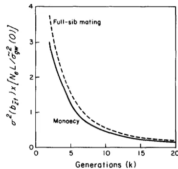
Generations ( k )
FIGURE 2.-Minimum sampling variance for the regression of phenotypic means on generation number for a neutral quantitative character in a finite population, shown for increasing numbers of consecutive generations. Note that regression analysis requires that k 2 2. Measurement error of the means is assumed to be negligible. The actual, expected sampling variance is obtained by multiplying the plotted values by G&(O)/N,L. Results are given for ideal monoecious populations and for full-sib mating.
tions. T h e standard least-squares expression for the regression coefficient is
k k
bit = [ q t )
-
.](t-
:)/E
( t-
t)’
(12)c=o C=O
where i is the mean phenotype averaged over all lines and generations. T h e expected value of bit is zero under the assumption of neutral additive genes. T h e expected sampling variance of bit may be written as
.;(t,t’)/L ( 1 3)
under the assumption that the sampling variance of the grand mean ( i ) is negligible. Substitution of Equa- tions 9-1 l shows that the sampling variance of bit is attributable to four causes: the genetic variance among initial line means, the variance and covariance of genotypic means resulting from drift, the sampling variance of means due to segregational variance, and the sampling variance of means due to environmental effects. While Equation 13 applies to the special case in which means are available for k
+
1 consecutive generations, the entire approach can be generalized to situations in which means are missing for some generations. This requires only that the proper vari- ance and covariance expressions be substituted for the ;:(t,t’) in Equation 13.M. Lynch
798
0.6
0.5
\ 0.4
I&
\ -0 \ 0.3
.
b
\
.
\
2
cb0.2
0. I
0 5 10 15 20
Generations ( k )
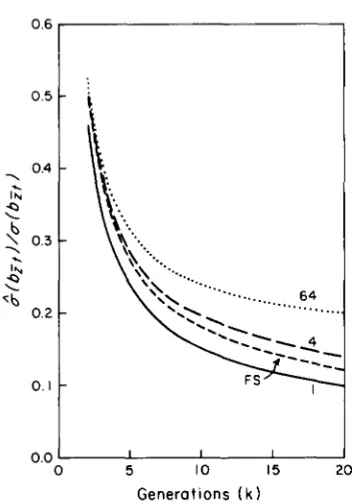
FIGURE 3,”Standard error for the regression coefficient b;,
under the assumption of bivariate normality and independent sam- pling relative to the true expectation. Results are given for ideal
monoecious populations of three effective sizes and for full-sib
mating.
offspring of the founders so that the large sampling variance of the founder means can be avoided. In that case, a2(b;,) is directly proportional to the genetic variation in the base population and inversely propor- tional to N,L. When means are available for only the first three generations
(k
= 2), a2(bi,) is not less than 3Z&(0)/NeL. With increasing numbers of generations, it declines exponentially. By dividing the plotted val- ues by NeL and taking the square root, it is possible to gain some appreciation of the magnitude of regression coefficients that are compatible with random genetic drift. For example, when data are available for 10 generations for a single full-sib mated line, a*(b;,)/ a&(O) 0.67/2.5 = 0.27. T h e standard error of bit in units of initial genetic standard deviations is therefore at least 0.5. Since the presence of environmental variation and finite sample size can cause further error, in this case a regression coefficient within the range*
Zgw(0) certainly would be compatible with a neutral hypothesis.I t is instructive to examine the bias in the sampling variance that would arise if one were to rely on the standard expression, &*(bit) = Z:(1
-
p2)/(k+
1 ) ~ :which is obtained under the assumption of independ- ent sampling and bivariate normality. Under the neu- tral hypothesis, the expected correlation p between
i ( t ) and t is zero, and for
k
+
1 consecutive samples, ( k+
1)a: = k(k+
l ) ( k+
2)/12. T h e sampling variance of the means over the experiment, Z:, can be ex- pressed in terms of Equations 9- 1 1.Ratios of the standard errors, & ( b i t ) / a ( b i t ) , for the
case in which measurement error is negligible and consecutive means are available starting with the off- spring of the founders, are given in Figure 3. T h e bias in the traditional estimator of the standard error of a regression coefficient is clearly too large to be ignored. Initially, a(bi,) is on the order of twice &(bit), and this factor increases severalfold with increasing numbers of generations.
Tests for inbreeding depression: While the proce- dures outlined above provide a means of evaluating whether a temporal sequence of mean phenotypes is consistent with the neutral additive gene hypothesis, a rejection of the null hypothesis should not be mis- construed as acceptance of the hypothesis of natural selection. When nonadditive interactions exist within and/or between loci, inbreeding can cause a shift in mean phenotypes in the absence of counterbalancing selection. The most common experimental design em- ployed in the detection of inbreeding depression is to subject a series of isolated lines to a regular program of inbreeding. T h e consecutive line means are then regressed on the expected inbreeding coefficient,
k k
b s = [Z(t)
-
Z ] [ F ( t )-
F ] / C
[ F ( t )-
F]’
(14)t=O t=O
where
F
is the mean expected inbreeding coefficient over the experiment. Such an analysis suffers from the same difficulties noted previously. T h e mean phe- notypes obtained from consecutive samples of the same line are not independent. Moreover, the distri- bution of F ( t ) is highly skewed, eventually piling up at values very close to one.T h e sampling variance of b;F under the neutral
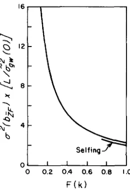
additive model can be computed by use of the proce- dures outlined above. Figure 4 provides the results for the special case in which environmental sources of variance are of negligible importance and the analysis begins with the founder ( F = 0) generation. When viewed as a function of the expected inbreeding in the final experimental generation, a*(b;F) depends very little on the effective population size. However, with larger N e , it takes longer to reach a given degree of inbreeding, and hence in early generations the results from selfed or full-sib mated lines are much more reliable than those from larger lines. The sam- pling variance of b i F is very high if the cumulative
inbreeding is less than 0.25, and diminishes to a min- imum of approximately
2.3Z&(O)/L
once inbreeding has proceeded beyond F = 0.9. Thus, relatively large departures from the expectation b i F = 0 can arise in inbreeding experiments even in the absence of domi- nance. Suppose, for example, that full-sib mating is performed on 10 lines for 10 generations ( F = 0.86). T h e sampling variance of b;F is then approximatelyAnalysis of Drift and Inbreeding 799
0 0.2 0.4 0.6 0.8 1.0
F ( k )
FIGURE 4.--Sampling variance of the regression o f mean phe- notype on the expected inbreeding coefficient under the assump- tion of neutral, additive gene action. The major curve applies to
full-sib mating and all cases of monoecy except selfing. The plotted values are minimum estimates as they d o not include variance from environmental variation or finite sample size. F ( k ) is the expected
level of inbreeding in the final generation of an experiment. The actual, expected sampling variance is obtained by multiplying the plotted values by Z&,(O)/L.
It is again useful to consider the bias that is incurred by using the standard expression for the variance of a regression coefficient as has been done in existing studies. Using the approach outlined above and fo- cusing on the special case in which environmental sources of variance can safely be ignored, it is seen in Figure 5 that the bias depends primarily on the du- ration of the experiment and very little on population size. T h e usual standard error, G(biF), always under- estimates the preferred measure a b i F . T h e bias in- creases with the experimental duration, asymptoting at & , / a b , = 0.25 beyond 20 generations.
As a rough check of the validity of conclusions on inbreeding depression derived from regression analy- sis, the statistic J = Ib;~I/2[6v,(o)/L]”, where 4 rep- resents the plotted values in Figure 4, may be useful. I f J exceeds one, the observed regression coefficient deviates from zero by more than two estimated stand- ard errors, and one is justified in suspecting the pres- ence of inbreeding depression. Of course, the true standard error of b;F cannot be known with certainty since the additive genetic variance in the base popu- lation is an estimate. The expectation of [6V,(O)/L]” will also be less than the true standard error of biF since measurement error has been ignored, but the bias should be small if the number of families and offspring within families assayed is large.
Estimates of biF/V$(O) are given for several species and characters in Table 2. Not all of the reported experiments were designed like the scenario pre- sented previously. However, almost all of the values of b;F/V$(O) are in excess of one and three exceed
0
-0 5 I O 15 20 25 Generat ions ( k 1
FIGURE 5,”Ratio of the standard error of b s based on normal regression theory relative to the expectation under random genetic drift. The upper curve applies to dioecious and monoecious popu- lations with Ne > 1.
five. Most of the data sets to which the J statistic may be applied are in strong agreement with the inbreed- ing depression hypothesis. For example, for yield in corn, L = 248,
6
= 2.1, and biF/Vg(O) = -3.27,yielding J = 17.8. However, it is questionable whether there is inbreeding depression for thorax length in Drosophila (J = 0.9), offspring number in Tribolium ( J
= 1.2), and internode length in barley (J = 0.2).
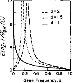
The magnitude of inbreeding depression suggested by Table 2 is fully compatible with a Mendelian model without epistatic interactions. For single loci, l b i F I / i?,(O)
>
1 will arise with complete dominance when recessive alleles have frequency c 0 . 3 , and with over- dominance, this condition is met over a broad range of gene frequencies (Figure 6). In theory, there is no upper bound to lbiFl/i?p(0) since in the case of over- dominance there is always a gene frequency at which there is no additive genetic variation, all of it appear- ing in the dominance component.In closing this section, another popular method of testing for inbreeding depression should be men- tioned. Frequently, the mean phenotypes from a sin- gle generation of a control and contemporaneous inbred population are compared by use of a standard t test or analysis of variance. This procedure seems indefensible since the expected variance of an inbred population exceeds that of the control. Moreover, the differences that can arise between control and inbred line means as a consequence of random drift as op- posed to inbreeding depression are ignored.
800 M. Lynch
TABLE 2
Results from various inbreeding experiments involving the regression, bZh of mean phenotype on expected inbreeding coefficient
Species Character Ref. L Ne F(k) b s 6;FlV&(O)
Mouse Litter size 1 , 2 10-6 2.5 0.63 -5.10 -3.64
3 20 2.5-32 0.95 -3.86 -2.74
3-week weight (9) 3 20 2.5-32 0.95 -2.54 -3.25
8-week weight (g) 3 20 2.5-32 0.95 -4.94 -2.63
Postweaning gain (9) 3 20 2.5-32 0.95 -2.18 -1.77
Sheep Clean fleece weight (Ib) 4
-
- 0.28 -4.4 -6.07Staple length (cm) 4
-
-
0.28 -1.2 - 1 .soBody weight (Ib) 4
-
- 0.28 -29.1 -6.29D. melanogaster Wing length (pm) 5 20 2.5-12 0.98 -34.8 -1.77
6 10 2.5-4 0.75 -52.0 -1.82
Thorax length (pm) 6 10 2.5-4 0.75 -16.8 -1.02
Abdominal bristle number 7 20-17 2.5 0.99 +1.82 +1.08
T. castaneum Offspring number 8 48 10-100 0.64 -2.56 -0.66
Barley Internode length 9 7 1 0.99 -2.36 -0.29
Corn Plant height (cm) 10 248 1 0.99 -48.0 -3.73
1 1 , 1 2 60 1-2.5 0.94 -55.4 -3.21
Ear height (cm) 10 248 1 0.99 -30.0 -2.83
1 1 , 1 2 60 1-2.5 0.94 -26.9 -1.69
Ear-leaf width (cm) IO 248 1 0.99 - I .34 -1.38
Ear length (cm) 10 248 1 0.99 -4.40 -3.69
Ear diameter (cm) 10 248 1 0.99 -10.08 -5.10
Kernel depth (mm) 10 248 1 0.99 -6.47 -4.69
Yield (g/ha) 10 248 1 0.99 -44.9 -3.27
Days to silking 10 248 1 0.99 +4.6 +1.19
L = number of lines, Ne = effective population size (in some cases several treatments were utilized), F(k) = maximum level of inbreeding
at the end of the experiment, V g ( 0 ) = additive genetic standard deviation in the base population. The work with sheep did not involve
discrete lines, but utilized members of a large population at various levels of inbreeding.
References: 1) BOWMAN and FALCONER (1960), 2) ROBERTS (1960), 3) EISEN and HANRAHAN (1974), 4) MORLEY (1 954), 5) TANTAWY and
REEVE (1956), 6 ) TANTAWY (1957), 7) KIDWELL and KIDWELL (1966), 8) RICH etal. (1984), 9) BATEMAN and MATHER (1951). 10) HALLAUER
and SEARS (1973), 11) CORNELIUS and DUDLEY (1974), 12) CORNELIUS (1972).
> Gene Frequency, q
FIGURE 6,"Expected standardized inbreeding depression
caused by a single diallelic locus with various dominance coefficients
( d ) and gene frequencies (4). Following standard theory (FALCONER
1981) and letting the three genotypic values at a locus be 2a, (1
+
d)a, and 0, it can be shown that E(6iF) = 2pqad and g&(O) = 2pqa2
[1 +
-
pH2.pling. Using Equation 9, it can be shown that the sampling variance is
(3/4);&(0)
+
2a:n
when the inbred progeny are acquired by self-fertil- ization, and
when they are acquired by full-sib mating.
These formulas are difficult to implement unless one has information on the components of variance in the base population. If, however, a single offspring is monitored from each family, then n = 1, and the preceding expressions become
a :
; = +[2G:(O) 1
+
(3/4);&(0)] Lwhere Z:(O) is the phenotypic variance in the random- bred population. Since the additive genetic variance is less than the phenotypic variance, these two quan- tities can be no greater than (1 1/4)2:(0)/L and (171 8)Z:(O)/L, respectively.
Analysis of Drift and Inbreeding 801
c
12
.
4
4 -
2
0
-0 20 40 60
c
N e
neous mating, and from each of these families measure a single random offspring. Then compute the statistic
where V,(O) is the observed phenotypic variance of random-bred progeny and 4 = 11/4 with self-fertiliz- ation and 17/8 with full-sib mating. Provided the character is approximately normally distributed, t may be treated as t-distributed with L
-
1 degrees of freedom. Suppose, for example, that the experiment consisted of 10 inbred and 10 random-bred families. Rejection of the null hypothesis of no inbreeding depresson at the 95% level then requires that t > 2 . 2 6 . For self-fertilization and full-sib mating, A i would have to exceed 1.2 and 1.0 phenotypic standard de- viations respectively for this criterion to be met.In the case of self-compatible plants that produce multiple flowers, the construction of diallels can fur- ther increase the power of a short-term test of inbreed- ing depression. Pairs of parent plants ( A and B ) can be used to produce two reciprocal outcrosses ( A X B and B X A) and two inbreds ( A X A and B X B ) . In this case, A i is the difference between the mean phe- notypes of offspring from the two types of mating. An advantage of this approach is that it eliminates the contribution of maternal effects and parent sampling to ui-. If n of each progeny type are obtained from each of L pairs of parents,
Even with n = 1, this quantity is less than Gz(O)/L. Thus, a very conservative test for inbreeding depres- sion using diallels is to maximize L , measuring one of each of the four types of progeny per parent pair, and then to employ Equation 16 with 4 = 1.
Analysis of the between-line variance: Regression analysis can be applied profitably to temporal data on
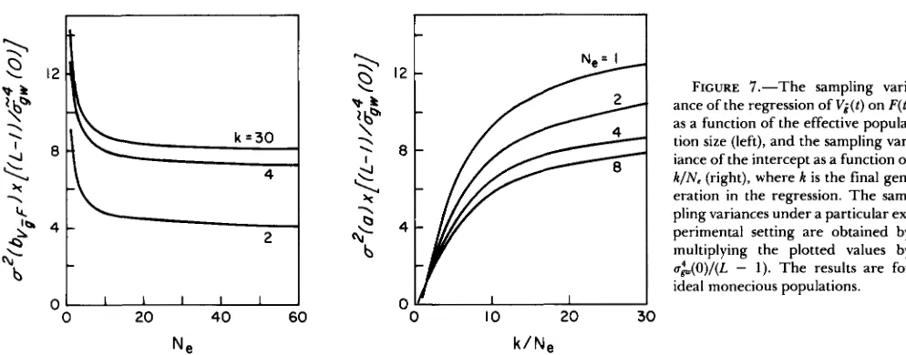
FIGURE 7.-The sampling vari- ance of the regression of V i ( t ) on F ( t ) as a function of the effective popula- tion size (left), and the sampling var- iance of the intercept as a function of k / N . (right), where k is the final gen- eration in the regression. The sam- pling variances under a particular ex- perimental setting are obtained by multiplying the plotted values by u&(O)/(L - 1). The results are for ideal monecious populations.
IO 20 30
k / N e
variances as well as on means. T h e regression of the between-population variance on the cumulative in- breeding ( b ~ p ) , for example, is a useful test of drift theory since its expectation is 2GL(O) for additive genes. T h e intercept of such a regression ( a ) is also of interest since, in the case of neutrality, it provides a pooled estimate of the between-line variance attrib- utable to factors other than drift (measurement error). Following the procedures outlined above,
U 2 ( b V i F ) =
1
I k
e
[F(t)-
F 1 2 )c
c
( E [ F ( t )-2 k k
t=O -0 1’=0
-
F ] E [ F ( t ’ )-
F]u[uj(t),uj(t’)]+
E[F(t)-
Vi]E[Vi(t’)-
V&J[F(t),F(t’)]],(17)
-
F]E[Vi(t’)-
V&[F(t),uz(t’)]+
E[V&t)n k k
where
Vi
is the mean between-line variance over an experiment ofk
+
1 consecutive generations, u[F(t), u j ( t ’ ) ] = 2u&(O)X‘”‘u~(t)/(L-
l), and u[F(t),F(t’)] =X*”‘&t)/(L
-
1) with t I t ’ . T h e variance of bvf has been derived under the assumption that the variance ofVi
is of negligible significance and ignores the variance of V i ( t ) due to measurement error. There- fore, Equations 17 and 18 give lower bounds on the sampling variances of the regresson parameters under the assumption of neutrality.T h e solution of Equation 17 indicates that u2(bvf) increases approximately twofold with the duration of the experiment, although it is essentially stable for
k
L 4 provided most pairs of loci are unlinked (Figure 7). For largek,
the standard error of bviF is no less than 3.8;&,(0)/(L - 1)” for self-fertilizing lines and 2&G&(O)/(L-
1)” for large Ne. For small Ne andk/
802 M. Lynch
"0 0.05 0.10 0 I5 0.20
3001 / / I
2 5 4 I'
%
I
300
...
0 0.08 0.16 0.24 0.32 0.40
1
0 002 004 0.06 0.08 0.10
lnbreedtng Coefflcient, F
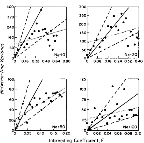
FIGURE 8.-Observed levels of between-line variance for pupal
weight for Tribolium populations at four effective sizes (RICH et al.
1984) as a function of the expected level of inbreeding (solid points).
Solid lines are the expected regressions under the neutral, additive genetic hypothesis; dashed lines are conservative 90% confidence limits; and dotted lines are the least-squares regressions.
than 0.9Z&(0).[k/Ne(L
-
l)]'*. With increasing k/N,, .*(a) gradually approaches a value on the order of.*(bv;F).
As an example of the application of the preceding formulas, the results of a large drift experiment with laboratory cultures of Tribolium castaneum (RICH et al. 1984) will be examined. T h e authors followed 12 replicate populations at four population sizes (1 : 1 sex ratio, random mating) over 20 consecutive genera- tions. Each generation, the mean pupal weight (pg) of each population was obtained from a bulk sample of 100 random individuals. The additive genetic vari- ance was estimated to be 460 in the base population. The observed V i ( t ) are plotted as a function of F ( t ) in Figure 8 , along with the expected divergence 920F(t) (solid lines). Any interpretation of the results of this study is weakened by the lack of a control. T h e authors argued that the downward trend in V i ( t ) in the last few generations of three of the four treatments was due to the suppression of random drift and the operation of stabilizing selection. However, the same result could have arisen as a response to a shift in the laboratory environment that influenced the expres- sion of variation.
T h e dashed lines in Figure 8 give the limits of the between-line variance beyond which there is a less than 5% chance for the realization of the drift process in either direction. Since these bounds are based on a
x*
distribution, which underestimates the dispersion somewhat, and also ignore measurement error, they may be regarded as conservative confidence limits. Nevertheless, almost all of the observations, with theTABLE 3
Least-squares estimates of the regression coefficients and intercepts for the data in Figure 8
IV, bv,, u ( b V l f ) a .(a)
10 148 412 109 154
20 222 402 91 87
50 312 396 21 3 8
100 292 394 28 19
T h e standard errors were obtained from Equations 17 and 18 under the assumption of unlinked loci.
exception of the late generations at N , = 10 and 20, lie within these limits. There are substantially more observations below (54) than above (26) the expecta- tion, possibly because the additive genetic variance in the base population was overestimated somewhat.
The least-squares regressions of the data are given by the dotted lines in the figure. The slope of each regression is less than the expected 920, but all are within 2 SE of the expectation (Table 3). The inter-
cepts are all above the expectation of zero, perhaps due to measurement error, but are well within 2 SE of
it. Thus, this fairly conservative analysis indicates that the observed patterns, even in the absence of a con- trol, are consistent with a hypothesis of random drift of neutral, additive genes. There is a significant prob- ability that the observed delines in V&t) late in the experiment arose by chance. In the case of the two smallest effective population sizes the chances of V&t) returning toward the expectation late in the experi- ment were small since the lines must have already become fixed at many loci.
STATISTICAL PROPERTIES O F T H E W I T H I N - POPULATION GENETIC VARIANCE
As in the case of the between-line variance, there are several reasons why the realized dynamics of the within-line variance may depart substantially from the expectation even when the assumptions of neutrality and additivity are met: variation in the genetic vari- ance among founder populations, variance in inbreed- ing, deviations from Hardy-Weinberg equilibrium, and linkage disequilibrium. Although substantial the- oretical progress on these matters has been made (AVERY and HILL 1977, 1979; BULMER 1976, 1980), the existing work relies on several simplifying assump- tions in the interest of analytical tractability: a base population in linkage equilibrium, no variance in in- breeding between populations, and t
<
2N,. Since the latter two assumptions will often be violated in empir- ical studies, it is necessary to relax them. The follow- ing analysis will focus on unlinked loci, since for most organisms the majority of pairs of loci are expected to be on different chromosomes.Analysis of Drift and Inbreeding 803
opment of linkage disequilibrium that inevitably de- velops in finite populations, even for unlinked loci. From AVERY and HILL (1 977), with two alleles/locus,
n n
a2[a&(t)l = 4
C
C
a,2a;[qio(l-
qio)qjo(li=l j = 1
-
qjo)]($qt+
2 4 ,
-
[I-
F(t)12)/L (19)where q,o is the initial gene frequency at the ith locus,
Bqt = E(D$t)/[qio(l
-
qio)qjo(l-
qjo)], and D$t is the squared linkage disequilibrium between loci i and j .An analytical expression is available for &it in CROW
and KIMURA (1970), whereas Oiir = 0. T h e two-locus expectations, $qf and Q,, are independent of gene frequencies and can be evaluated by use of the mo-
ment-generating matrix of HILL and ROBERTSON
( 1 968), which applies to systems of invariant inbreed- ing. T o accommodate variance in inbreeding, a Tay- lor expansion was performed on the elements of the matrix, letting a2(N,)
=
&1)/4F(l).Obviously, Equation 19 is a rather complicated function, but great simplification can be gained fol- lowing the logic of AVERY and HILL (1977). First, note that the squared expectation of the within-pop- dation variance is
$tjt = E [ q i t ( 1
-
q t t ) q I t ( 1-
qjt)]/[qio( 1-
qio)qjo( 1-
q j o ) ] ,n n
g&(t) = 4
C C
a?a,2[qio(1-
qi0)qjOr = l , = I
Second, note that the fraction of terms in Equations
19 and 20 attributable to pairs of loci is ( n
-
l)/n, so that with large numbers of loci the contribution of single-locus terms becomes diminishingly small. Thus, the squared coefficient of variation isThis function is plotted for ideal monoecious popula- tions and for full-sib mating in Figure 9. T h e pre- dicted variance is that which is expected within a large progeny group.
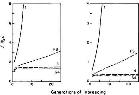
For populations of effective sizes of 4 or greater,
r
4 / 3 N e L from the very outset of an experiment. The same conclusion was reached by AVERY and HILL (1977), showing that for unlinked loci, their results hold very well even for large t/Nc and are influenced only negligibly by variance in inbreeding. T h e results of BULMER (1980), obtained in a different manner, suggestr may be closer to
5/3NeL, but this discrep- ancy has little bearing on the following conclusions. For smaller populations, the variance in &(t) caused by linkage is somewhat larger. With full-sib matingr
rises from 0.5/L to 0.8/L by 10 generations of in- breeding, at which point it would be very difficult to acquire accurate estimates of a&(t) since inbreeding8 1
-
6 -
-
FS
/ / *
/ C C 0 -
4
I..-
.-..-..-.-..-..-.-:
64O . ' l I l
0 10 2 0
Generotions of Inbreeding
FIGURE 9.-The sguared coefficient of variation of the within-
population genetic variance multiplied by N e t , considering only the
variation caused by linkage disequilibrium. The panel on the left
refers to a large progeny group after the denoted generations of
inbreeding; the panel on the right refers to the situation after the progeny group has been mated randomly for a single generation.
has proceeded to 90%. With self-fertilization,
r in-
creases from 2.0/L to 6.3/L at five generations of inbreeding.Since linkage disequilibrium is a transient phenom- enon, the sampling variance of u&(t) can be reduced substantially by expanding and randomly mating within each line prior to analysis. T h e improvement in accuracy can be determined by recomputing $ol
and Oyt from the moment-generating matrix after al- lowing for an additional generation with (1/2N,)
=
0. T h e results of a single generation of such treatment are shown in Figure 9, where it can be seem that r isreduced to between 50% and 25% of its previous value if the loci are unlinked.
Several other sources of variation of a&(t) exist. First, there is the variance in the initial within-line variance caused by a finite number of founders. If the lines are established with independent members of the base population, then a'[a&(O)] = 2g&(0)/L(Nm