Some Recent Developments in Parametric and Nonparametric Regression Models.

(1)

ABSTRACT

LIN, CHEN-YEN. Some Recent Developments in Parametric and Nonparametric Regression Models. (Under the direction of Hao Helen Zhang and Howard D. Bondell.)

(2)

c

(3)

Some Recent Developments in Parametric and Nonparametric Regression Models

by Chen-Yen Lin

A dissertation submitted to the Graduate Faculty of North Carolina State University

in partial fulﬁllment of the requirements for the degree of

Doctor of Philosophy

Statistics

Raleigh, North Carolina

2012

APPROVED BY:

Leonard A. Stefanski Yichao Wu

Hao Helen Zhang

Co-chair of Advisory Committee

Howard D. Bondell

(4)

BIOGRAPHY

(5)

ACKNOWLEDGEMENTS

First of all, I want to take this opportunity to express my great appreciation to my advisors Dr. Hao Helen Zhang and Dr. Howard D. Bondell. I beneﬁt so much from their profound insight into statistics and their professionalism. Helen and Howard have been very generous and patient to me. I feel extremely fortunate to have them as my thesis advisors.

My sincere thanks also go to Dr. Leonard A. Stefanski and Dr. Yichao Wu for joining my committee and providing many suggestions on my research. I wish to thank other faculty members in the statistics department for their excellent lectures.

Finally, special thanks to all the friends I love and friends who love me from Taiwanese Student Association. The journey will be so much less colorful without you.

“Faithful friends are a sturdy shelter: whoever finds one has found a treasure.” (Sirach

(6)

LIST OF TABLES

Table 1.1 Summary of area under ROC and PR curves . . . 13

Table 2.1 Elapsed CPU time for solving COSSO-QR model . . . 34

Table 2.2 Simulation result for Example 1 with independent features . . . 35

Table 2.3 Simulation result for Example 1 with dependent features . . . 36

Table 2.4 Simulation result for Example 2 with independent features . . . 37

Table 2.5 Simulation result for Example 2 with dependent features . . . 38

Table 2.6 Estimated prediction risk for real data . . . 38

Table 3.1 Elapsed CPU time for solving NPLSA procedure . . . 54

Table 3.2 NPLSA result for quantile regression with independent features . . 55

Table 3.3 NPLSA result for quantile regression with dependent features . . . 55

Table 3.4 NPLSA result for Logistic regression with independent features . . 56

(9)

LIST OF FIGURES

Figure 1.1 Empirical selection probabilities plot . . . 14

Figure 1.2 Condition numbers plot for simulation Example 2 . . . 15

Figure 1.3 Averaged ROC curves for simulation Example 1 . . . 15

Figure 1.4 True positives plot for simulation Examples 3 . . . 16

Figure 1.5 MSPE curve as a function of model size . . . 16

Figure 2.1 Estimated functions and conﬁdence band . . . 34

Figure 3.1 Degrees of freedom decomposition. . . 54

Figure 3.2 Solution paths for real data . . . 57

(10)

Chapter 1 Refining Forward Selection in

High-Dimensional Feature Space by

Perturbation

1.1 Introduction

We consider a high-dimensional linear regression model

yi =β1x (1)

i +. . .+βpx (p)

i +εi, i= 1, . . . , n, (1.1)

where yi is the response, xi = (x (1) i , . . . , x

(p)

i ) is a p-dimensional vector of predictors, p ≫n, and εi is the random error with mean zero and ﬁnite variance. We assume that the response and each predictor are centered so there is no intercept in (1.1).

(11)

The majority of variable selection methods revolve about the notion of selection con-sistency and examine how often a method identiﬁes the correct model. However, in the modern world of high-dimensional data, a scientist does not expect to identify the correct predictors with no mistakes. In many instances, a scientist would simply prefer a properly ranked list of candidate predictors and hope that the important ones would tend to be ranked at or near the top of the list. Our goal is to obtain a ranked list whose ordering improves upon the ordering obtained by the existing methods. As also remarked by Xin and Zhu (2012), the task of ranking is the most fundamental. Once the variables are ranked, from a decision-theoretic framework, the choice of thresholding has more to do with one’s belief on the tradeoﬀ between false positives and false negatives.

For any selection procedure that generates a ranked list or a sequence of candidate models, such as forward selection or penalized regression, despite many information cri-teria having been proposed, it remains a highly debated topic how to pick a ﬁnal model from the selection path. Even in the traditional large n small p situations, the correct model may not be an element in the selection path (Leng et al., 2006; Wang, 2009), making selection consistency less realistic in the high-dimensional case. More discussion on the selection consistency of penalized regression methods can be found in Zhao and Yu (2006) and Fan and Lv (2010) and references therein. When selection consistency is not feasible, a pertinent alternative is to study if a selection procedure possesses the sure screening property, i.e. all important predictors would be included with probability going to one (Fan and Lv, 2008).

In this study, we revisit a classic yet popular selection procedure, forward selection (FS). Recently, Wang (2009) studied the sure screening property of FS and showed the-oretically and numerically that FS can consistently detect all important predictors even if the number of predictors is substantially larger than the sample size. Despite that FS enjoys such desirable property, the method has several limitations. For instance, resulting from its greedy search algorithm, FS tends to eliminate other informative predictors if they are correlated with the ones that are in the current model (Efron et al., 2004). In a high-dimensional setup, Donoho and Stodden (2006) showed that there exists a break-down point for standard model selection procedures including FS and LASSO (Tibshirani, 1996, 2011) when the number of variables exceeds the sample size. Moreover, both FS and LASSO can only identify at mostn predictors before it saturates whenn ≪p.

(12)

mini-mand perturbation of Jin et al. (2001), we propose a computationally-intensive method, which we call the perturbed FS. The notion of minimand perturbation is originally in-troduced to derive the sampling distribution of some parameter estimates in parametric models. In this work, we explore the perturbation technique in order to enhance the sta-bility in variable selection. Our perturbation method is reminiscent of a weighted least squares (WLS), as it can be viewed as randomly weighting the observations. With ran-dom weights, the WLS method bears some similarity with Bayesian bootstrap (Rubin, 1981) and Bayesian Bagging (Clyde and Lee, 2001).

Compared to the original FS, the main advantage of the proposed method is that: the new method no longer depends on a greedy search hence can better handle corre-lated predictors and identify more predictors than sample size. More importantly, as we demonstrate later in the article, the perturbed FS provides a competitive, and often su-perior, variable ordering and prediction accuracy. Obviously the price we pay is increased computational intensity. However, as will be explained later, the procedure involves ap-plying FS to multiple perturbed data and the implementation of the procedure does not require communication between diﬀerent tasks and therefore can be facilitated by taking advantage of parallel computing (Knaus et al., 2009).

Our proposed method is based on repeatedly applying FS on multiple perturbed data and produces an aggregated importance indicator for each predictor. This philosophy has a close proximity to a higher-level notion of variable-selection ensemble (VSE) (Xin and Zhu, 2012). Ensemble methods were originally proposed in the machine learning literature, such as bagging (Breiman, 1996) and random forests (Breiman, 2001). More recently, ensemble methods have become popularized in the variable selection context, for example, random LASSO (Wang et al., 2011) and stability selection (Meinshausen and B¨uhlman, 2010). Both methods conceptually generate many bootstrap samples and apply LASSO algorithm repeatedly to produce a more stable and powerful procedure. Thus, Random LASSO, stability selection and our perturbed FS can all be viewed as diﬀerent manifestations of VSE.

(13)

1.2 Forward Selection

Let{(yi,xi), i= 1, . . . , n}, be the observed random sample from a population where the relationship betweenyi andxican be described through a linear function in (1.1). Denote M={j1, . . . , jp∗}as the model containingx

(j1) i , . . . , x

(jp∗)

i as relevant predictors and|M| as the cardinality of the set. Further denote the true model as MT ={j :βj ̸= 0}where we assume |MT|=p0 ≪p.

1.2.1 Forward Selection Path

The original forward selection algorithm can be summarized in the following steps

Step 0: (Initialization) SetS(0) ₌_{∅}_.

Step 1: In thek-th step (k ≥1), for allj ∈ {1, . . . , p}\S(k−1)_{, consider a candidate model} S(k−1)_∪{_j_}_{and compute its sum of squared error SSE}(k−1)

j . Identify which predictor results in the smallest sum of squared error, say jk

∗ = arg min j∈{1,...,p}\S(k−1)

SSE(_jk−1). Then update the model at the k-th stepS(k) =S(k−1)∪ {j_∗k}.

Step 2: Increase loop indexk by 1 and go back to Step 1 until k =n.

(14)

1.2.2 Perturbed Forward Selection Path

To generate multiple perturbed datasets, one popular method is the bootstrap. How-ever, bootstrap-type methods suffer from some immediate difficulties when n < p. For instance, bootstrapping residuals is not practical since all residuals are zeros. Moreover, nonparametric bootstrap will produce less thann unique observations, making the num-ber of identifiable predictors less than n, and can in fact be much less. More recently, Meinshausen and Bühlman (2010) proposed a stability selection procedure which ran-domly chooses a subsample of sizen/2 as a method to stabilize the LASSO penalization. This method has the limitation that the number of recoverable predictors becomes n/2. Due to the limitations of bootstrap and related data perturbation methods, we con-sider an alternative by perturbing the objective function as in Jin et al. (2001). In the least squares context, the objective function we aim to minimize is given by

min

β (y−Xβ)

T_W₍_y₋_Xβ₎_, _(1.2)

where W = diag(w1, . . . , wn) is a diagonal matrix containing weights for each observa-tion. The original unperturbed data would have W = I. We adopt a random weight generated from an underlying distribution F(w), which can be viewed as a perturbation to the objective function. In principle, any non-negative random variable can be used as weight and, as remarked in Jin et al. (2001), the solution is robust to the choice of distribution function. Diﬀerent choices ofF(·) allows us to make several interesting analo-gies to existing methods. For instance, when F(·) is the Bernoulli distribution function with success probability 0.5, i.e. we expect to retain n/2 observations, the perturbation method is closely related to aforementioned stability selection. We propose, instead, to consider a continuous weight, more speciﬁcally, the exponential weight. When F(·) is the distribution function of an exponential random variable, it is essentially the same as assigning a random Dirichlet weight to each observation, giving some resemblance to Bayesian Bootstrap (Rubin, 1981) and Bayesian bagging (Clyde and Lee, 2001).

Although we initiate the new method from perturbing the objective function, the WLS problem in (1.2) is equivalent to an OLS problem by multiplying each obser-vation by its corresponding square root of the weight. Thus, as an equivalent formu-lation, we consider a multiplicative perturbation method to generate B datasets. Let

(15)

dataset by (y_i(b),x(_ib)) =

√

w_i(b)(yi,xi). After generating B perturbed datasets, we apply the aforementioned FS algorithm on each of them and store its saturated modelS(n)₍_b_).

Denote ˆπj = B−1

∑B

b=1I(j ∈ S

(n)₍_b₎₎_{, j} _{= 1}_{, . . . , p}_{, as the empirical probability of}

se-lecting the j-th predictor among B perturbations, then the perturbed FS path is given by ranking the empirical selection probabilities in a descending order.

The computation cost depends on the number of perturbed datasets and a naive programming algorithm is sequentially applying FS on each of them. In light of the fact that this procedure does not require communication between the FS computations but performs each task separately, a sophisticated yet efficient programming technique is to take advantage of parallel computing. Most commercially available computers nowadays are equipped with two to eight processing cores. To fully exploit the devices, an efficient algorithm should reduce to multiple parallel tasks, each accessing a specific dataset. We implemented a parallel computing algorithm to accelerate the procedure in R using the snowfall package (Knaus et al., 2009). The supporting R code is available from the authors upon request.

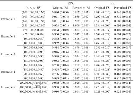
To visually show the eﬀectiveness of data perturbation, we use a microarray exper-iment of Scheetz et al. (2006) as a motivating example. This gene expression dataset consists of 120 arrays, each array contains 31,042 probe sets (Aﬀymetric GeneChip Rat Genome 230 2.0 Array). The complete gene expression data is available at Gene Ex-pression Omnibus (http://www.ncbi.nlm.nih.gov/geo; accession number GSE5680). The primary objective of this study is to identify which gene expressions are related to that of gene TRIM 32, which is recently found to cause Bardet-Biedl syndrome (Chiang et al., 2006).

(16)

3 unpermuted genes out of 8. However, after a reasonable number of perturbations, most of the unpermuted genes stand out and the separation between permuted and unper-muted genes becomes clear toward the end. This encouraging ﬁnding justiﬁes the use of perturbation method to achieve better variable ordering in a high-dimensional feature space.

We give a formal description of the perturbed FS and the computational algorithm here. The perturbed FS algorithm can be summarized in the following steps.

Step 0: Initialization. Set S_P(0) ={∅}.

Step 1: In thek-th step (k ≥1), identify the predictor with the largest empirical selec-tion probability, say j_k∗ = arg max

{1,...,p}\Sp(k−1)

ˆ

πj. Then update the model at the k-th step

S(k)

p =Sp(k−1)∪ {j_k∗}.

Step 2: Increase loop indexkby 1 and go back to Step 1 until all predictors are included in the path, i.e. k=p.

Considering the ﬁnite number of perturbations may not guarantee an unique maxi-mum in Step 1, there are two types of situations that needs special treatments, including

Case 1: (ˆπj = ˆπk > 0, for some j, k): We break the tie by the average step they enter the FS. For a given perturbed path that selects the j-th predictor, we not only know j ∈ S(n)(b) but the step it is included. Thus, we let the j-th predictor enter the perturbed path ﬁrst if, in average, it takes fewer steps to enter each perturbed path.

Case 2: (the set {j : ˆπj = 0}is not empty): We break the tie by the magnitude of their marginal correlations with the response. The larger the absolute correlation, the earlier it enters the perturbed FS path.

(17)

in the order of tens of thousands. For a reasonable number of perturbations, we adopt the tie-breaking technique as introduced before to save computation cost.

By construction, of several major diﬀerences between the original FS and the per-turbed FS, one of which is the traditional FS path can only rank the most important

n predictors; whereas the perturbed path provides a comprehensive rank for all p pre-dictors. For fair comparison, for those predictors which are not selected by the original FS, we rank them according to their marginal correlations and then append the ordered path into the original FS path so that both of the original FS and perturbed paths have length p.

1.3 Numerical Study

1.3.1 Simulation Models

In this section, we demonstrate the perturbed FS and compare it to the original FS using simulations. Five diﬀerent examples are considered in this study.

Example 1 (Independent Features): We start from an example that is similar to the one used in Fan and Lv (2008). There are p = 1000 predictors and p0 = 10

non-zero coefficients. Each predictor is independently generated from standard nor-mal distribution. The first p0 coefficients are non-zero and are given by βj = (−1)Uj_{(4 log}_n/√_n ₊|_Z

j|), j = 1, . . . , p0, where Uj follows a Bernoulli distribu-tion with success probability 0.4 and Zj is another independent random variable following a standard normal distribution.

Example 2 (Autoregressive): Following a similar setting as that in Example 1, we let

p= 1000 andp0 = 8 but the correlation between predictors having an autoregressive

structure with pairwise correlation cor(x(_ij), x(_ik)) = 0.7|j−k|_, _∀_j _̸₌_k_{. Similarly, the} ﬁrst p0 coeﬃcients are non-zero and generated in the same fashion as before.

(18)

Example 4 (Factor Model): This example is based on Meinshausen and B¨uhlman (2010) withp= 1000 andp0 = 4. Letϕ1, ϕ2 be two latent factors that independently come

from N(0,1). Then each predictor xij is generated as xij =fij,1ϕi1+fij,2ϕi2+ηij, wherefij,1, fij,2andηij havei.i.d.standard normal distributions for allj = 1, . . . , p. The four locations of non-zero coeﬃcients are randomly chosen and the coeﬃcients are generated from uniform (0,1).

Example 5 (Diverging parameters): In the previous examples, the true model sizes are fixed. We consider a different situation wherep0 diverges with the sample size (Zou and Zhang, 2009). More specifically, we adopt the similar setup as Example 1 but letp= 5000 and p0 =⌊

√ n⌋.

In Examples 1-4, we consider two sample sizes and two theoretical R2 ₌ Var(xiβ)

Var(yi)

com-binations. As for Example 5, we ﬁx R2 _{= 0}_._{6 and vary the sample size. Later we use the}

notation (n, p, p0, R2) to denote the combination of sample size, number of predictors,

number of non-zero coeﬃcients and theoretical R2. Regarding the number of perturba-tions, the exploratory experiment shown in Figure 1.1 suggests the selected probability stabilizes moderately fast. So we use B = 200 in the simulation. We also tried B = 300, but the results were comparable. We run each simulation scenario 100 times and report the summary statistics and their associated standard error.

To evaluate the quality of variable ordering, considering the candidate model at each step of the selection path, we compute the true positives, the number of informative pre-dictors included in the current step, and the false positives, the number of noise prepre-dictors included in the current step. The receiver operating characteristic (ROC) curve, which plots the true positive rate against the false positive rate, or equivalently the sensitivity against one minus speciﬁcity, on a two-dimensional plane, is a common tool to illustrate the relationship between type I error and power.

(19)

1.3.2 Simulation Result

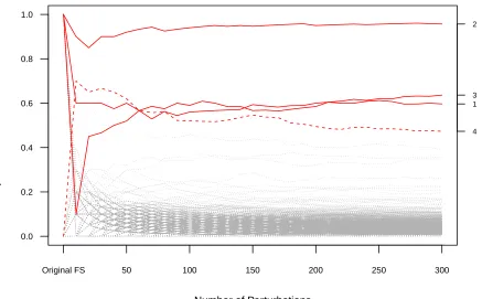
Based on the simulation result summarized in Table 1.1, the perturbed FS evidently outperforms the original FS across all scenarios. In Examples 1 and 5, the area under PR curve suggests as large as 30% improvement can be achieved by using the perturbed FS. In Examples 2-4, where we consider correlated predictors, greater improvement can be expected. This observation is coherent with the theoretical property of the original FS. The greedy algorithm hinders other prominent predictors from entering the selection path because of their correlation with the ones that are already included in the current model. This greedy nature can be illustrated in Figure 1.2. In Figure 1.2, we demonstrate how the condition number of the design matrix changes with the model size in the second simulation example. Since the original FS tends to include an additional predictor which is less correlated to those in the current model, it naturally leads to a design matrix with relatively smaller condition number.

Complementary to a point summary given in Table 1.1, Figure 1.3 provides a com-prehensive visual comparison between these two competing methods. Shown in Figure 1.3 are averaged ROC curves over 100 simulated data in Example 1 with n = 150 and

R2 _{= 0}_._{5. As can be seen from the left panel, the ROC curve of the perturbed FS}

com-pletely dominates that of the original FS, particularly when specificity is greater than 0.3. When specificity becomes less and less, the separation between these two lines quickly vanishes, which is the reason why their area under ROC curves do not differ by a large margin as that in the area under PR curve. Nonetheless, when specificity is 0.6, it im-plies the model size is around 400, which is not feasible since sample size is only 150. In practice, our attention is usually drawn toward the beginning of the path or a more practical model size. In the right column of the plot is the same ROC curve but zoom in the region where specificity is greater than 0.9, or model size is less than 100. In the region of interest, the effectiveness of perturbed FS becomes transparent. Therefore, it is clear that most improvement of our new method comes from a better variable ranking in the beginning of the path.

(20)

perturbed FS provides superior ranking.

1.3.3 Real Data

To examine the real data application, we analyzed two microarray datasets: the rat array (Scheetz et al., 2006) and the inbred mouse array (Lan et al., 2006). The rat array is described in Section 1.2.2. The inbred mouse data consists of 60 arrays, 31 female and 29 male mice, and each array measures the expression values of 22,690 genes. A continuous phenotypic variables measured by RT-PCR, stearoyl-CoA desaturase 1 (SCD1), is used as the response.

We ﬁrst screen down the number of genes to 2,000 and 1,999, respectively, using sure independent screening (Fan and Lv, 2008). For the inbred mouse data, we also include gender as an additional predictor so both datasets consist of 2,000 potential predictors.

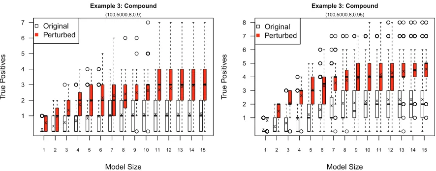
The performance of our perturbed FS algorithm is compared to the original FS using out-of-sample prediction. To assess prediction accuracy, we ﬁrst split the data into two folds, training and testing sets, accounting for 80% and 20% of the full data, respectively. We apply the original FS and perturbed FS algorithm on the training set and estimate regression parameters each step of the paths, then apply the estimated model parameters on the testing set and evaluate the mean squared prediction error (MSPE). This process will be carried out 100 times and averaged.

In Figure 1.5, we compute the MSPE from model sizes 1 to 40. In addition, the MSPE from the null model, the model without any predictor, is also provided in the plot as a baseline performance. From Figure 1.5, the MSPE of the perturbed FS is signiﬁcantly better than that of the original FS in both datasets. The performance is similar in small model sizes, suggesting both methods can identify some strong signals in the beginning. However, the original FS can not continue to identify useful predictors to improve prediction accuracy.

1.4 Discussion

(21)

success-fully alleviates several limitations of the original FS. The number of identiﬁable variable is no loner limited by the sample size as that in the original FS. Moreover, the ordered variable list has the power to rank important predictors ahead of those irrelevant ones. Simulation studies suggest that the perturbed FS has superior selection path than the original FS, and the real analysis of two microarray datasets shows the sound prediction performance in practice.

(22)

Table 1.1: Average area under ROC and PR curves in 5 simulation examples over 100 runs. The standard error is given in the parentheses.

ROC PR

(n, p, p0, R2) Original FS Perturbed FS Original FS Perturbed FS

Example 1

(100,1000,10,0.50) 0.846 (0.006) 0.867 (0.007) 0.263 (0.016) 0.346 (0.015)

(100,1000,10,0.80) 0.971 (0.004) 0.989 (0.002) 0.792 (0.021) 0.839 (0.012)

(150,1000,10,0.80) 0.891 (0.005) 0.932 (0.005) 0.540 (0.020) 0.606 (0.014)

(150,1000,10,0.80) 0.998 (0.001) 1.000 (0.000) 0.984 (0.004) 0.993 (0.002)

Example 2

(75,1000,8,0.50) 0.833 (0.012) 0.854 (0.012) 0.326 (0.017) 0.425 (0.023)

(75,1000,8,0.80) 0.906 (0.008) 0.947 (0.007) 0.569 (0.022) 0.694 (0.022)

(100,1000,8,0.80) 0.842 (0.011) 0.896 (0.009) 0.404 (0.017) 0.507 (0.021)

(100,1000,8,0.80) 0.952 (0.006) 0.978 (0.004) 0.750 (0.019) 0.816 (0.018)

Example 3

(100,5000,8,0.90) 0.884 (0.005) 0.890 (0.008) 0.089 (0.010) 0.300 (0.017)

(100,5000,8,0.95) 0.915 (0.005) 0.961 (0.004) 0.170 (0.021) 0.521 (0.019)

(150,5000,8,0.90) 0.928 (0.004) 0.974 (0.003) 0.243 (0.021) 0.598 (0.019)

(150,5000,8,0.95) 0.983 (0.003) 0.998 (0.001) 0.533 (0.025) 0.926 (0.009)

Example 4

(150,1000,4,0.50) 0.738 (0.014) 0.767 (0.016) 0.269 (0.023) 0.351 (0.027)

(150,1000,4,0.80) 0.868 (0.012) 0.887 (0.012) 0.613 (0.028) 0.695 (0.025)

(200,1000,4,0.50) 0.766 (0.015) 0.824 (0.014) 0.383 (0.030) 0.467 (0.028)

(200,1000,4,0.80) 0.899 (0.011) 0.917 (0.009) 0.725 (0.024) 0.817 (0.017)

Example 5

(200,5000,⌊√200⌋,0.60) 0.932 (0.004) 0.929 (0.005) 0.482 (0.018) 0.545 (0.014)

(400,5000,⌊√400⌋,0.60) 0.958 (0.003) 0.979 (0.002) 0.778 (0.012) 0.800 (0.010)

(23)

Number of Perturbations

Empir

ical Selection Probabilities

4 1 3 2

Original FS 50 100 150 200 250 300

0.0 0.2 0.4 0.6 0.8 1.0

(24)

Model Size C o n d . N u mb e r

1 5 10 15 20

1 2 3 4 5 (100,1000,8,0.5)

Example 2: Autogressive

Original FS Perturbed FS Model Size C o n d . N u mb e r

1 5 10 15 20

1 2 3 4 5 (150,1000,8,0.5)

Example 2: Autogressive

Original FS Perturbed FS

Figure 1.2: Condition number at diﬀerent model sizes in simulation Example 2. The solid line and broken line represent the perturbed FS and the original FS, respectively.

0.0 0.2 0.4 0.6 0.8 1.0

0 .2 0 .4 0 .6 0 .8 1 .0 1−Specificity Se n si ti vi ty

Example 1: Independent Features

(100,1000,10,0.5)

0.00 0.02 0.04 0.06 0.08 0.10

0 .2 0 .4 0 .6 0 .8 1 .0 1−Specificity Se n si ti vi ty

Example 1: Independent Features

(100,1000,10,0.5)

(25)

Model Size T ru e P o si ti v e s x x x x x x x x x x x x x x x x x x x x x x x x x x x x x x

1 2 3 4 5 6 7 8 9 10 11 12 13 14 15

1 2 3 4 5 6 7 (100,5000,8,0.9)

Example 3: Compound

Original Perturbed Model Size T ru e P o si ti v e s x x x x x x x x x x x x x x x x x x x x x x x x x x x x x x

1 2 3 4 5 6 7 8 9 10 11 12 13 14 15

1 2 3 4 5 6 7 8 (100,5000,8,0.95)

Example 3: Compound

Original Perturbed

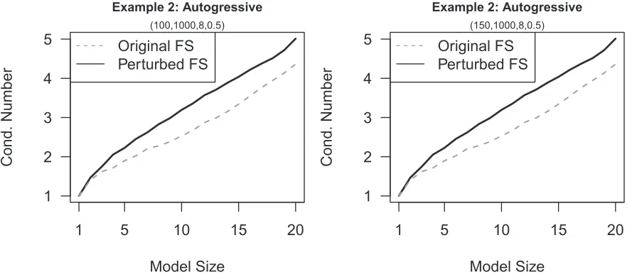
Figure 1.4: True positives at diﬀerent model sizes in Examples 3. The white box and red box represent the original FS and perturbed FS, respectively. Cross sign represents the average over 100 runs. The left panel is theR2 _{=0.90 and the right panel is the}_R2 _=0.95.

Inbred Mouse Array

Model Size MSPE ● ● ●● ● ● ● ●●_● ●●●●●●●●●●●●●●●●●●●●●●●●●●●● ●● ● 0.5 1.0 1.5 2.0

1 10 20 30 40

● Original FS Perturbed FS Rat Array Model Size MSPE ● ● ● ● ● ● ● ●●●●_{●●●●●●●●●●●●●●}●●●●●●●●●●●●●●●● 0.010 0.015 0.020

1 10 20 30 40

(26)

Chapter 2 Variable Selection for

Nonparametric Quantile Regression

via Smoothing Spline ANOVA

2.1 Introduction

Quantile regression, as a complement to classical least square regression, provides a more comprehensive framework to study how covariates inﬂuence not only the location but the entire conditional distribution (Koenker, 2005). In quantile regression problems, the primary interest is to establish a regression function to reveal how the 100τ% quantile of the response y depends on a set of covariates x = (x(1)_{, . . . , x}(p)_{). A parametric form of}

regression function is often assumed for convenience of interpretation and lower compu-tational cost. While a linear regression function is studied in Koenker and Bassett (1978) and numerous follow-up studies, Procházka (1988) and Jure˘cková and Procházka (1994) explored nonlinear regression; see Koenker and Hallock (2001) and Koenker (2005) for a comprehensive overview.

(27)

func-tion can be found via solving the minimizafunc-tion problem

min f∈F

n

∑

i=1

ρτ(yi−f(xi)) +λV(f′), (2.1)

where ρτ(·) is the so-called “check function” of Koenker and Bassett (1978),

ρτ(t) = t[τ−I(t <0)], τ ∈(0,1), (2.2)

λis a smoothing parameter andV(f′) is the total variation of the derivative off. Koenker et al. (1994) showed that the minimizer is a linear spline with knots at the design points

xi, i = 1, . . . , n, provided that the space F is an expanded second-order Sobolev space deﬁned as

F =

{

f :f(x) = a0+a1x+

∫ 1

0

(x−y)+dµ(y), V(µ)<∞, ai ∈R, i= 0,1

}

, (2.3)

whereµis a measure with ﬁnite total variation. Bloomﬁeld and Steiger (1983) and Nychka et al. (1995) considered a similar problem as that in (2.1), but used a smoothing spline penalty

min f∈F

n

∑

i=1

ρτ(yi−f(xi)) +λ

∫

[f′′(x)]2dx. (2.4)

The minimizer of (2.4) over a second-order Sobolev space is a natural cubic spline with all design points as knots. Bosch et al. (1995) proposed an interior point algorithm which is proven to converge to solve the minimization problem.

For multi-dimensional feature space, He et al. (1998) proposed a bivariate quantile smoothing spline and He and Ng (1999) generalized the idea to multiple covariates us-ing an ANOVA-type decomposition. Li et al. (2007) proposed a more general framework called the kernel quantile regression (KQR). By penalizing the roughness of the func-tion estimator using its squared funcfunc-tional norm in a reproducing kernel Hilbert space (RKHS), the KQR solves the regularization problem

min f∈HK

n

∑

i=1

ρτ(yi−f(xi)) + λ

2||f||

2

HK, (2.5)

(28)

Fenske et al. (2011) proposed a boosting method to select and estimate additive quantile function. Although their method was not intentionally targeting at variable selection, with moderately small number of iterations, boosting algorithm naturally achieves vari-able selection by using the most important predictors to update the ﬁtted function.

Despite several existing nonparametric quantile function estimators, selecting relevant predictors in multi-dimensional data is an important yet challenging topic that has not been addressed in depth. Variable selection in quantile regression is much more diﬃcult than that in the least square regression. The variable selection is carried at various levels of quantiles, which amounts to identifying variables that are important for the entire distribution, rather than limited to the mean function as in the least squares regression case. This has important applications to handle heteroscedastic data. Several regularization methods were proposed (Zou and Yuan, 2008a,b; Wu and Liu, 2009) for linear quantile regression. However, to our knowledge, there still lacks a method for variable selection in nonparametric quantile regression. This is the main motivation of our work.

(29)

The remainder of the article is organized as follows. Section 2 reviews the SS-ANOVA models and introduces the new estimator. An iterative computation algorithm is given in Section 3, along with parameter tuning procedure. Extensive empirical studies, including both the homogeneous and heterogenous errors are given in Section 4. Three real example analysis results are presented in Section 5. We conclude our ﬁndings in Section 6.

2.2 Formulation

2.2.1 Smoothing Spline ANOVA

In the framework of smoothing spline ANOVA (SS-ANOVA), it is assumed that a function

f(x) = f(x(1)_{, . . . , x}(p)_{) has the ANOVA decomposition} f(x) =b+

p

∑

j=1

fj(x(j)) +

∑

j<k

fj,k(x(j), x(k)) +· · · , (2.6)

whereb is a constant,fj’s are the main eﬀects andfj,k’s are the two-way interactions, and so on. We estimate each of the main eﬀects in a RKHS denoted byHj ={1}⊕H¯j whereas the interactions are estimated in a tensor product spaces of the corresponding univariate function spaces. When x(j) is a continuous variable, a popular choice ofHj is the second-order Sobolev space S2[0,1] = {g : g, g′ are absolutely continuous and g′′ ∈ L2[0,1]}. When endowed with the norm

||g||2 =

{∫ 1

0

g(x)dx

}2

+

{∫ 1

0

g′(x)dx

}2

+

∫ 1

0

{g′′(x)}2dx, (2.7)

the second-order Sobolev space is a RKHS with reproducing kernel

R(x, y) = 1 +k1(x)k1(y) +k2(x)k2(y)−k4(|x−y|), (2.8)

wherek1(x) = x−₂1,k2(x) = 1₂

[

k4 1(x)−

1 12

]

andk4(x) = ₂₄1

[

k4 1(x)−

1 2k

2 1(x) +

7 240

]

. When

x(j) _{is a categorical variable that takes only ﬁnite distinct values,} _{₁_{, . . . , L}_}_{, we use a}

diﬀerent reproducing kernel

(30)

See Wahba (1990) and Gu (2002) for more details. The entire tensor-product space for estimating f(x) is given by

F =⊗p_j=1Hj ={1} ⊕ p

∑

j=1

¯

Hj ⊕

∑

j<k

( _¯

Hj⊗H¯k

)

⊕ · · · . (2.10)

Note that F = ⊗p_j=1Hj is also a RKHS, and its reproducing kernel is the sum of the reproducing kernels of those component spaces.

In practice, the higher-order interactions in (2.6) will usually be truncated for con-venience in interpretation and to avoid the curse of dimensionality. A general expression for a truncated space can be written as

F ={1} ⊕ F1 ={1} ⊕{⊕q_j₌₁Fj

}

, (2.11)

where F1, . . . ,Fq are q orthogonal subspaces of F. A special case is the well-known additive model (Hastie and Tibshirani, 1990) withq =p, in which only the main effects are kept in the model, sayf(x) =b+∑_jd₌₁fj(x(j)). When both main effects and two-way interaction effects are retained, the truncated space has q =p(p+ 1)/2. For illustration purpose, we focus on the additive model afterward in this paper, thus all the interactions are dropped. But the idea can be naturally generalized to any function space with higher order interactions.

A typical method for estimating nonparametric quantile function is through solving the regularization problem

min f∈F

1

n n

∑

i=1

(31)

2.2.2 New Methodology: COSSO-Quantile Regression

To achieve joint variable selection and function estimation in nonparametric quantile regression, we consider the following regularization problem

1

n n

∑

i=1

ρτ(yi−f(xi)) +λ p

∑

j=1

wj||Pjf||, (2.13)

where wj’s are known weights. We will refer to (2.13) as COSSO-QR afterward.

The problem in (2.13) is a ﬂexible modeling framework that includes several existing methods as special cases. For instance, it reduces to the L1-norm quantile regression (Li

and Zhu, 2008) in linear models. More speciﬁcally, if f(x) = b +∑_jp₌₁βjx(j) and we consider a linear functional space F = {1} ⊕ {⊕p_j₌₁{x(j)−1/2}} with inner product

⟨f, g⟩ = ∫ f g, then the RKHS norm penalty ||Pjf|| becomes proportional to |βj|. We allow each functional component to be penalized diﬀerently depending on its associated weight wj ∈ (0,∞). In principle, smaller weights are assigned to important function components while larger weights are assigned to less important components. This is in the same spirit of the adaptive LASSO (Zou, 2006) and adaptive COSSO (Storlie et al., 2011). We propose to construct the weights wj from the data adaptively. For each component fj, its L2-norm ||fj(x)||L2 =

√∫

[fj(x)]2dF(x), F(·) is the distribution function of x, is a natural measure to quantify the importance of functional components. In practice, given a reasonable initial estimator ˜f, we propose to construct the weights

w’s by its inverse empirical L2-norm

w_j−1 =||Pjf˜||n,L2 =

v u u

t_n−1

n

∑

i=1

[Pj_f˜₍_x

i)]2, j = 1, . . . , p. (2.14)

A convenient choice of ˜f is the solution of the KQR.

Due to the fact that both the check loss and the penalty functionalJ(f) are continuous and convex in f, the existence of the minimizer of (2.13) is guaranteed as stated in the following Theorem.

Theorem 1. Let F be an RKHS of functions with the decomposition (2.11), then there exists a minimizer to (2.13) in F.

(32)

di-mensional space F for a minimizer is practically infeasible. Analogous to the smoothing spline models, the following Theorem shows that the minimizer of (2.13) lies in a ﬁnite dimensional space. This important result assures the feasibility of computation.

Theorem 2. Representer Theorem: Let the minimizer of (2.13) be fˆ = ˆb +∑p_j₌₁fˆj

with fˆj ∈H¯j, then fˆj ∈span{RFj(x

(j)

i ,·), i= 1, . . . , n} where RFj(·,·) is the reproducing kernel of Fj.

2.3 Algorithm

To further facilitate the computation, we ﬁrst present an equivalent formulation of (2.13). By introducing non-negative slack variables θj, j = 1, . . . , p, and using the Lemma 2 in Lin and Zhang (2006), it is easy to show that minimizing (2.13) is equivalent to solving the following optimization problem

min f,θ 1 n n ∑ i=1

ρτ(yi−f(xi)) +λ0 p

∑

j=1

w2_jθ_j−1||Pjf||2

s.t. p

∑

j=1

θj ≤M, θj ≥0,∀j,

(2.15)

whereλ0 andM are both smoothing parameters. The roles of the slack variables θj’s are very diﬀerent from those in smoothing splines model. The slack variables θj’s allow us to recover the sparse structure sinceθj = 0 if and only if||Pjf||= 0 (Lin and Zhang, 2006). Moreover, when θj’s are unknown, the penalty part in (2.15) reduces to that in tradi-tional smoothing spline and thus by the Representer Theorem of Kimeldorf and Wahba (1971), the minimizer of (2.15) has the form

f(x) = b+ n

∑

i=1

ciRθ,w(xi,x), (2.16)

where c= (c1, . . . , cn)∈Rn, b∈R, and Rθ,w =

∑p

j=1w− 2 j θjRFj.

LetRj ={RFj(x

(j) i , x

(j) i′ )}

n

i,i′=1be ann×nmatrix and1nbe a column vector ofnones. When evaluated the minimizer at the design points, we write f = (f(x1), . . . , f(xn)) as

f = b1n+ (

∑p

j=1w− 2

j θjRj)c and deﬁne ||v||Cτ = n−

1∑n

(33)

n. The objective function in (2.15) becomes

min b,c,θ

y−b1n−

( _p ∑ j=1 θj w2 j Rj ) c Cτ

+λ0cT

( _p ∑ j=1 θj w2 j Rj ) c s.t. p ∑ j=1

θj ≤M, θj ≥0, ∀j.

(2.17)

For the remaining of the article, we will refer to (2.17) as the objective function of our proposed method.

2.3.1 Iterative Optimization Algorithm

It is possible to minimize the objective function in (2.17) with respect to all the pa-rameters, (b,cT_,_θT₎T_{, simultaneously, but the programming eﬀort can be substantial.} Alternatively, we can decompose the parameters into two parts,θ and (b,cT₎T_{, and then} iteratively solve two sets of optimization problems in turn, with respect toθand (b,cT₎T_. Consequently, we suggest the following iterative algorithm:

1. Fix θ, solve (b,cT)T min

b,c

y−b1n−

( _p

∑

j=1 θj w_j2Rj

) c Cτ

+λ0cT

( _p

∑

j=1 θj w2_jRj

)

c. (2.18)

2. Fix (b,cT₎T_{, solve} min

θ ∥y

∗₋_Gθ_∥

Cτ +λ0c

T

Gθ, s.t. p

∑

j=1

θj ≤M, θj ≥0, ∀j, (2.19)

where y∗ = y − b1n and G = {g1, . . . ,gp} is an n × p matrix with columns

g_j =w_j−2Rjc.

(34)

In practice, based on our empirical experience, the algorithm converges quickly in a few steps. We have noted that the one-step solution often provides a satisfactory approx-imation to the solution. As a result, we advocate the use of one-step update in practice. An important connection between our proposed method and the KQR can be un-raveled by realizing that the objective function in (2.18) is exactly the same as that in the KQR. This connection suggests that when θ is known, our proposed method shares the same spirit as the KQR. The optimization problem for estimating θ essentially im-poses the non-negative garrote (Breiman, 1995) type shrinkage onθ’s, and hence achieves variable selection by shrinking some of θj’s to zero.

2.3.2 Parameter Tuning

Like any other penalized regression problem, the performance of the new estimator criti-cally depends on properly-tuned smoothing parameters in (2.17). Smoothing parameters play an important role in balancing the trade-oﬀ between the goodness of data ﬁt and the model complexity. A reasonable parameter choice is usually the one that minimizes some generalized error or information criterion. In the quantile regression literature, one com-monly used criterion is the Schwarz information criterion (SIC) (Schwarz, 1978; Koenker et al., 1994)

log

(

1

n n

∑

i=1

ρτ(yi−fˆ(xi))

)

+logn

2n df, (2.20)

wheredf is a measure of complexity of the fitted model. Various authors (Koenker, 2005; Yuan, 2006; Li et al., 2007) have argued using the number of zero residuals as an estimate of effective degrees of freedom. In our experimental study, we realized the estimated degrees of freedom fluctuates a lot among different smoothing parameters and therefore may lead to an unstable tuning result. As an alternative, we consider a bootstrap method which will be presented in the following section to estimate the degrees of freedom.

In addition to the SIC, another popular criterion to choose the smoothing parameter isk-fold cross validation, which has been widely applied to various regression and classi-ﬁcation problems and usually gives competitive performance. In the following numerical study, we will report the result for both SIC and 5-fold cross validation.

(35)

Step 1. Initialization. Set θj = 1, ∀j.

Step 2. For each of the grid points of λ0, solve (2.18) for (b,cT)T, and record the SIC

score or CV error. Choose the best λ0 that minimizes the SIC or CV error, then

ﬁx it in later steps.

Step 3. For each of the grid points of M, solve (2.17) for (b,cT_,_θT

)T _{using the} afore-mentioned iterative optimization algorithm. Record the SIC score or CV error at each grid point and choose the bestM that minimizes either SIC score or CV error.

Step 4. Solve (2.17) using the chosenλ0 and M pair, on the full data. Note that this is already done if tuning was based on SIC.

Since the tuning procedure described above does not cover all the possible pairs of (λ0, M), it would be beneﬁcial to enhance the tuning with a reﬁned search. In particular,

we suggest to do the following. After Step 3, say, we obtain the optimal pair (λ∗₀, M∗). Then we focus on a narrowed and more focused region, the neighborhood of (λ∗₀, M∗) and apply Step2 and 3 again. The optimal parameters determined at this refined step, say, (λ∗∗₀ , M∗∗) will be used as the final selection. Our simulation study also confirms that this refined tuning procedure can improve the prediction and selection performance substantially.

2.3.3 Bootstrapped Degrees of Freedom Estimate

In nonparametric quantile regression literature, using the number of zero residuals as a measure of model complexity has been widely adopted. The notion was originated from a more generic quantity, the divergence formula ∑n_i₌₁ ∂fˆ(xi)

∂yi , which ﬁrst appeared in

Stein’s unbiased risk estimation (SURE) (Stein, 1981) and later been extensively used to evaluate the eﬀective degrees of freedom for various modeling procedures, see Ye (1998), Efron (2004), Koenker (2005) and reference therein.

(36)

1. For a particular pair of smoothing parameters (λ0, M), ﬁt the COSSO-QR model

in equation (2.17) and store the ﬁtted values ˆfi and residualsri =yi−fˆi.

2. Repeat this step B times.

2.1. Generate a bootstrapped response

y_iboot = ˆfi +riboot, r boot i

iid

∼ _Fˆ_n₍_r₎_{, i}_{= 1}_{, . . . , n,} _(2.21)

where ˆFn is the empirical distribution function of the residuals.

2.2. Fit the COSSO-QR model but replace the original response by the boot-strapped response and record the ﬁtted values ˆf_iboot.

3. For each i= 1, . . . , n, ﬁt a simple linear regression model by regressing ˆfboot

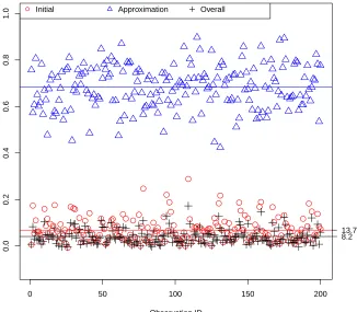
i onyiboot and use the estimated slope as an estimate of the derivative. Thus the bootstrapped degrees of freedom estimate is given by summing up then estimated slopes.

Estimating the derivative by regression slope was pioneered in Ye (1998). To better suit our quantile regression model, we generate perturbed response by bootstrapping rather than adding artificial noise to the observed response as used in Ye’s original pro-posal. As remarked by Ye (1998), different perturbation methods have minor influence on estimating the slope and will not lead to considerable bias.

2.4 Numerical Results

In this section we present the empirical performance of the COSSO-QR procedure us-ing simulated data. For the experiment design, we use the followus-ing functions as build-ing blocks: g1(t) = t; g2(t) = (2t− 1)2; g3(t) =

sin(2πt)

2−sin(2πt) and g4(t) = 0.1 sin(2πt) +

0.2 cos(2πt) + 0.3 sin2(2πt) + 0.4 cos3(2πt) + 0.5 sin3(2πt). Similar settings were also con-sidered in Lin and Zhang (2006).

(37)

as the selected model and true model, respectively, and|M| as the cardinality of the set

M. Then we compute four statistics for assessing selection accuracy: correct selection,

I( ˆM = M0, type I error rate, |M∩Mˆ c0|

p−|M0|, power,

|_M∩M0|ˆ

|M0| , and model size, |

ˆ

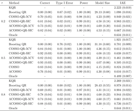
M|. For the purpose of comparison, we also include the solution of the KQR ﬁtted with only relevant predictors based on 5-fold cross validation tuning. This method will later be referred to as the Oracle estimator. The Oracle estimator provides a benchmark for the best possi-ble estimation risk if the important variapossi-bles were known. We also include two existing methods, the KQR and boosting QR (Fenske et al., 2011), for comparisons.

Another property that we would like to study is the role of the adaptive weights in the performance of the COSSO-QR procedure. Without any a priori knowledge on the importance of each predictor, we can set all wj = 1 in (2.13) and proceed to solve the objective function. For the adaptive proposal, we use the KQR as an initial estimate, ˜f, to produce an adaptive weight.

Three diﬀerent quantile valuesτ ={0.2,0.5,0.8}, are used throughout the simulation. For each of the following examples, we repeat 100 times and report the average summary statistics and their associated standard errors.

We consider two simulation models with detailed result given in Tables 2.2 to 2.5.

2.4.1 Computational Cost

Before introducing simulation models, we ﬁrst study how computationally intense our method is. To assess the computational cost, we present the average elapsed CPU times for solving equation (2.15) for a ﬁxed pair of (λ0, M) over 200 replicates. The predictors

x= (x(1)_{, . . . , x}(p)_{) are independently generated from}_U₍₀_,_{1) and then take}_n_observations

from the model

yi = 5g1(x (1)

i ) + 3g2(x (2)

i ) + 4g3(x (7)

i ) + 6g4(x (10)

i ) +ε, i= 1, . . . , n, (2.22)

where εi are independently drawn from t(3). We consider multiple sample size n and dimension p combinations. All computations are done on a desktop PC with an Intel Core i7-2600K CPU and 12GB of memory. The average CPU times are summarized in Table 2.1.

(38)

the computing time substantially increases from n = 100 to n = 300, but varies little between diﬀerent number of inputs and quantiles.

2.4.2 Homoskedastic Error Model

We ﬁrst consider generating response from a location family given in (2.22) and keep the error distribution unchanged. It follows that the 100τ% quantile function in the homoskedastic model is given by

Qτ(y|x) = 5g1(x(1)) + 3g2(x(2)) + 4g3(x(7)) + 6g4(x(10)) +Fε−1(τ), (2.23) whereFε(·) is the distribution function of ε. To examine the model selection of COSSO-QR, we generate predictors x(j)_{, j} _{= 1}_{, . . . ,}_{40, marginally from} _U₍₀_,_{1) and consider}

an autoregressive type of dependency by letting pairwise correlation cor(x(j)_{, x}(k)_{) =} ρ|j−k|_, ∀_j ̸₌ _k_{. Two levels of dependency will be used} _ρ ₌ {₀_,₀_.₇}_{. We use sample size} n = 200 in this case and present the performance of ﬁve competing procedures: KQR, boosting QR, COSSO-QR, adaptive COSSO-QR, and the Oracle estimator, in Table 2.2 and 2.3.

Another interesting observation can be made by examining the robustness property of the COSSO-QR in estimating the conditional median function. Although least squares regression and quantile regression are not generally comparable, the conditional median and mean functions coincide in this example, making the comparison between them jus-tiﬁable. Thus, we incorporate two sparse least squares nonparametric regression models, COSSO (Lin and Zhang, 2006) and adaptive COSSO (Storlie et al., 2011), to estimate the conditional mean function and see how our method compare with them.

(39)

for variable selection.

With regard to variable selection, the proposed COSSO-QR is eﬀective in identifying important variables and removing noise variables, particularly when using SIC as a tuning procedure, which is shown by its small Type I error and large power. The adaptive COSSO-RQ tends to select a slightly larger model size, thus increases both Type I error and power. Overall speaking, the COSSO-QR procedure shows promising performance in terms of both variable selection and quantile estimation in this example.

The conditional mean function estimators, COSSO and adaptive COSSO, give com-parable model selection. However, as can be seen from IAE, their estimations are seriously aﬀected by the heavy tail of the error distribution. Beneﬁted from their sparse property, they still perform better than KQR but are less competitive to the other procedures, even with adaptive weight. In addition, the standard errors are almost 10 tens larger than the other median estimators, implying our COSSO-QR method enjoys the robust property when median is of interest.

Figure 1 gives a graphical illustration for the fitted curve and pointwise confidence band given by the adaptive COSSO-QR for τ = 0.2. For comparison, the estimated functions by the Oracle are also depicted. We apply each procedure to 100 simulated datasets and a pointwise confidence band is given by the 5% and 95% percentiles. Figure 1 suggests that the COSSO-QR produces a very good estimation for the true functions, and the fits are comparable to those given by the Oracle estimator. The fourth function component is more difficult to estimate due to its subtle features in extreme values and inflexion points.

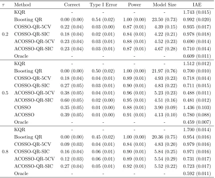
When predictors are correlated, Table 2.3 shows our procedure is slightly aﬀected. Overall, the type I error is well-controlled within 5% and the power is close to 90% most of the time. Moreover, the IAE suggests we do not lose too much eﬃciency relative to the Oracle estimator.

2.4.3 Heteroskedastic Error Model

To further examine the ﬁnite sample performance of the new methods, we consider gen-erating response from a location-scale family

yi = 5g1(x (1)

i ) + 3g2(x (2)

i ) + 4g3(x (7)

i ) + 6g4(x (10)

i ) + exp

[

2g3(x (12) i )

]

(40)

whereεi i.i.d.

∼ N(0,1). In the heteroskedastic model, the 100τ% quantile function is given by

Qτ(y|x) = 5g1(x(1)) + 3g2(x(2)) + 4g3(x(7)) + 6g4(x(10)) + exp

[

2g3(x(12))

]

Φ−1(τ), (2.25)

where Φ(·) is the distribution function of standard normal. The predictors are generated in the same fashion as that in the previous example and we use sample size n = 300 in this case.

From this example, we aim to evaluate the performance of the COSSO-QR under the scenario where some variables can only be inﬂuential on a certain range of quantiles. More speciﬁcally, like the homoskedastic example, the median function depends on the 1, 2, 7 and 10th predictors. However, other than the median function, x(12) _{will not only}

be inﬂuential but its eﬀect becomes larger and larger toward the tails.

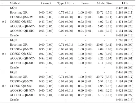
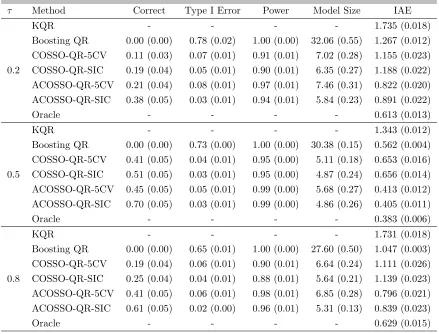
Table 2.4 and 2.5 summarize the performance of all competing methods. Again, we observe that the adaptive COSSO-QR performs the best and the KQR is the worst in terms of prediction error. However, the boosting QR provides as efficient or sometimes even more efficient estimation than the COSSO-QR. Similarly, for variable selection, by penalizing a more complicated model, SIC tuning procedure usually selects a smaller model size and identifies the correct model more frequently.

Another point we would like to emphasize is that when τ = 0.5, the estimated model size is close to 4 as expected, since the median only depends on the 1,4,7 and 10th predic-tors. When τ is away from 0.5, our COSSO-QR procedures can successfully identify the additional informative predictor in the error variance, suggesting that the new method’s capability to identify all the relevant predictors that inﬂuence the distribution of the response.

2.5 Real Data Analysis

(41)

daily ozone concentration and 8 meteorological covariates. The data has been used in various studies (Buja et al., 1989; Breiman, 1995; Lin and Zhang, 2006). These two data are publicly available in the R packages ElemStatLearn and cosso, respectively.

We apply our methods on these datasets and estimate the prediction risk, Eρτ(Y − f(X)), by randomly reserving 10% of the data as testing set. The smoothing parameters, tuned by 5-fold cross validation, and model parameters are estimated using only the training set. The estimated parameters will then be applied on the testing set and the prediction risk is used as a comparison between various methods. The entire procedure is repeated 100 times and averaged.

Table 2.6 summarizes the prediction risk along with its associated standard error. Based on the result, the adaptive weights is not always helpful in real application. The advantage of adaptive weight is more perceivable in the prostate data. But, with or without adaptive weight, the diﬀerences between them are usually within reasonable error margin. Overall, the key observation is that our proposed method provides competitive and usually superior prediction than the existing methods.

Apart from comparing prediction error, we also apply our methods to the complete prostate data and summarize variable selection. An interesting comparison is that in the study of mean function, Tibshirani (1996) selected three prominent predictors, log-cancer volume, log-weight and seminal vesicle invasion. These three predictors are also selected by our approach when we consider the median. However, in the 20% quantile, gleason score shows up as an additional predictor. Meanwhile, in the 80% quantile, only two predictors are chosen, cancer volume and seminal vesicle invasion, but not log-weight.

2.6 Conclusions

We propose a new regularization method that simultaneously selects important predictors and estimate the conditional quantile function. Our method is available in theRpackage cosso version 2.0-2. The COSSO-QR method conquers the limitation of selecting only predictors that inﬂuence the conditional mean in least square regression, facilitating the analysis of the full conditional distribution. The proposed method also includes the L1

(42)

selecting important predictors.

(43)

0.0 0.2 0.4 0.6 0.8 1.0 −3 −2 −1 0 1 2 x1 P 1f True Oracle ACOSSO−QR

0.0 0.2 0.4 0.6 0.8 1.0

−1 .5 −1 .0 −0 .5 0 .0 0 .5 1 .0 x2 P 2f

0.0 0.2 0.4 0.6 0.8 1.0

−2 −1 0 1 2 3 4 x3 P 3f

0.0 0.2 0.4 0.6 0.8 1.0

−4 −2 0 2 4 x4 P 4f

Figure 2.1: The ﬁtted function components and their associated pointwise conﬁdence band for homoskedastic example with independent features. The dark solid line is for the true function component, the light solid line is for the Oracle estimator and the broken line is for the adaptive COSSO-QR estimator.

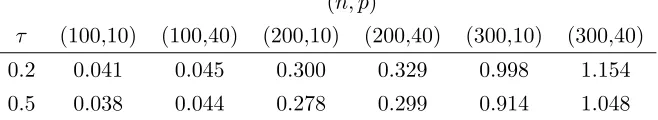
Table 2.1: Elapsed CPU time (in seconds) for solving COSSO-QR model.

(n, p)

τ (100,10) (100,40) (200,10) (200,40) (300,10) (300,40)

0.2 0.041 0.045 0.300 0.329 0.998 1.154

(44)

Table 2.2: Simulation results for the homoskedasitc example with independent fea-tures. The standard errors are given in the parentheses.

τ Method Correct Type I Error Power Model Size IAE

KQR - - - - 2.223 (0.019)

Boosting QR 0.00 (0.00) 0.67 (0.02) 1.00 (0.00) 28.13 (0.60) 1.098 (0.016)

COSSO-QR-5CV 0.70 (0.05) 0.01 (0.00) 0.98 (0.01) 4.23 (0.09) 0.949 (0.021)

0.2 COSSO-QR-SIC 0.81 (0.04) 0.02 (0.01) 0.99 (0.01) 4.58 (0.18) 0.983 (0.021)

ACOSSO-QR-5CV 0.73 (0.05) 0.02 (0.01) 0.99 (0.01) 4.69 (0.20) 0.645 (0.016)

ACOSSO-QR-SIC 0.82 (0.04) 0.02 (0.00) 1.00 (0.00) 4.53 (0.15) 0.667 (0.016)

Oracle - - - - 0.634 (0.011)

KQR - - - - 1.921 (0.017)

Boosting QR 0.00 (0.00) 0.76 (0.02) 1.00 (0.00) 31.18 (0.60) 0.781 (0.009)

COSSO-QR-5CV 0.84 (0.04) 0.01 (0.00) 1.00 (0.00) 4.36 (0.15) 0.612 (0.015)

COSSO-QR-SIC 0.92 (0.03) 0.00 (0.00) 0.99 (0.01) 4.08 (0.13) 0.638 (0.017)

0.5 ACOSSO-QR-5CV 0.82 (0.04) 0.01 (0.00) 1.00 (0.00) 4.39 (0.11) 0.461 (0.008)

ACOSSO-QR-SIC 0.93 (0.03) 0.00 (0.00) 0.99 (0.00) 4.07 (0.06) 0.505 (0.012)

COSSO 0.83 (0.04) 0.01 (0.00) 0.99 (0.01) 4.15 (0.05) 0.824 (0.025)

ACOSSO 0.76 (0.04) 0.01 (0.00) 0.99 (0.01) 4.30 (0.08) 0.616 (0.017)

Oracle - - - - 0.489 (0.007)

KQR - - - - 2.269 (0.021)

Boosting QR 0.00 (0.00) 0.68 (0.02) 1.00 (0.00) 28.43 (0.55) 0.978 (0.014)

COSSO-QR-5CV 0.69 (0.05) 0.01 (0.00) 0.97 (0.01) 4.31 (0.11) 0.904 (0.022)

0.8 COSSO-QR-SIC 0.78 (0.04) 0.02 (0.01) 0.98 (0.01) 4.68 (0.23) 0.944 (0.024)

ACOSSO-QR-5CV 0.74 (0.04) 0.02 (0.01) 0.99 (0.00) 4.60 (0.17) 0.661 (0.015)

ACOSSO-QR-SIC 0.88 (0.03) 0.01 (0.00) 0.99 (0.00) 4.30 (0.15) 0.726 (0.017)

(45)

Table 2.3: Simulation results for the homoskedasitc example with dependent features. The standard errors are given in the parentheses.

τ Method Correct Type I Error Power Model Size IAE

KQR - - - - 1.743 (0.015)

Boosting QR 0.00 (0.00) 0.54 (0.02) 1.00 (0.00) 23.50 (0.73) 0.992 (0.020)

COSSO-QR-5CV 0.22 (0.04) 0.03 (0.00) 0.87 (0.01) 4.39 (0.15) 0.935 (0.017)

0.2 COSSO-QR-SIC 0.18 (0.04) 0.02 (0.01) 0.84 (0.01) 4.22 (0.21) 0.978 (0.018)

ACOSSO-QR-5CV 0.23 (0.04) 0.03 (0.01) 0.88 (0.01) 4.52 (0.23) 0.690 (0.014)

ACOSSO-QR-SIC 0.23 (0.04) 0.03 (0.01) 0.87 (0.01) 4.67 (0.28) 0.710 (0.014)

Oracle - - - - 0.609 (0.011)

KQR - - - - 1.512 (0.012)

Boosting QR 0.00 (0.00) 0.50 (0.02) 1.00 (0.00) 21.97 (0.76) 0.700 (0.010)

COSSO-QR-5CV 0.18 (0.04) 0.04 (0.01) 0.89 (0.01) 4.93 (0.23) 0.718 (0.014)

COSSO-QR-SIC 0.27 (0.05) 0.03 (0.01) 0.90 (0.01) 4.83 (0.22) 0.711 (0.015)

0.5 ACOSSO-QR-5CV 0.38 (0.05) 0.04 (0.01) 0.96 (0.01) 5.23 (0.23) 0.488 (0.011)

ACOSSO-QR-SIC 0.60 (0.05) 0.02 (0.00) 0.95 (0.01) 4.51 (0.16) 0.481 (0.012)

COSSO 0.35 (0.05) 0.01 (0.00) 0.88 (0.01) 3.90 (0.09) 1.436 (0.103)

ACOSSO 0.39 (0.05) 0.01 (0.00) 0.91 (0.01) 4.13 (0.10) 0.780 (0.088)

Oracle - - - - 0.459 (0.007)

KQR - - - - 1.700 (0.014)

Boosting QR 0.00 (0.00) 0.45 (0.02) 1.00 (0.00) 20.36 (0.75) 0.954 (0.016)

COSSO-QR-5CV 0.09 (0.03) 0.04 (0.01) 0.84 (0.01) 4.83 (0.20) 0.979 (0.016)

0.8 COSSO-QR-SIC 0.16 (0.04) 0.06 (0.01) 0.90 (0.01) 5.84 (0.25) 0.971 (0.016)

ACOSSO-QR-5CV 0.12 (0.03) 0.06 (0.01) 0.89 (0.01) 5.54 (0.29) 0.731 (0.017)

ACOSSO-QR-SIC 0.27 (0.04) 0.05 (0.01) 0.92 (0.01) 5.52 (0.22) 0.723 (0.017)

Some Recent Developments in Parametric and Nonparametric Regression Models.

ABSTRACT

BIOGRAPHY

ACKNOWLEDGEMENTS

TABLE OF CONTENTS

LIST OF TABLES

LIST OF FIGURES

Chapter 1

Refining Forward Selection in

High-Dimensional Feature Space by

Perturbation

1.1

Introduction

1.2

Forward Selection

1.2.1

Forward Selection Path

1.2.2

Perturbed Forward Selection Path

1.3

Numerical Study

1.3.1

Simulation Models

1.3.2

Simulation Result

1.3.3

Real Data

1.4

Discussion

Chapter 2

Variable Selection for

Nonparametric Quantile Regression

via Smoothing Spline ANOVA

2.1

Introduction

2.2

Formulation

2.2.1

Smoothing Spline ANOVA

2.2.2

New Methodology: COSSO-Quantile Regression

2.3

Algorithm

2.3.1

Iterative Optimization Algorithm

2.3.2

Parameter Tuning

2.3.3

Bootstrapped Degrees of Freedom Estimate

2.4

Numerical Results

2.4.1

Computational Cost

2.4.2

Homoskedastic Error Model

2.4.3

Heteroskedastic Error Model

2.5

Real Data Analysis

2.6

Conclusions