Spectral methods to approximate the likelihood for irregularly spaced spatial data

Spectral methods to approximate the likelihood for irregularly spaced spatial data

Montserrat Fuentes

Mimeo Series 2568 -

Likelihood approaches for large irregularly spaced spatial datasets are often very difficult, if not infeasible,

to use due to computational limitations. Even when we can assume normality, exact calculations of the

likelihood for a Gaussian spatial process observed at n locations requiresO(n3) operations. We present a

version of Whittle’s approximation to the Gaussian log likelihood for spatial regular lattices with missing

values and for irregularly spaced datasets. This method requiresO(nlog₂n) operations and does not involve

calculating determinants. Due to the edge effect the estimated covariance parameters using this approximated

likelihood method are efficient only in one dimension. To remove this edge effect, we introduce data tapers.

In spatial statistics, data tapers are often the tensor product of two one-dimensional tapers. However, we

generally need more tapering for the corner observations. Thus, we introduce here a new spatial data taper,

a circular taper, that gives more tapering to the corner observations. Therefore, with less overall tapering,

we get the amount of smoothing that we need without losing so much information. We present simulations

and theoretical results to show the benefits and the performance of the data taper and the spatial likelihood

approximation method presented here for spatial irregularly spaced datasets and lattices with missing values.

1_{M. Fuentes is an Associate Professor at the Statistics Department, North Carolina State University (NCSU), Raleigh,} NC 27695-8203, and a visiting scientist at the US Environmental Protection Agency (EPA). Tel.:(919) 515-1921, Fax: (919) 515-1169, E-mail: [email protected].

1

Introduction

Statisticians are frequently involved in the spatial analysis of huge datasets. In this situations, calculating

the likelihood function, to estimate the covariance parameters or to obtain the predictive posterior density, is

very difficult due to computational limitations. Even if we can assume normality, calculating the likelihood

function involvesO(N3) operations, whereN is the number of observations.

However, if the observations are on a regular complete lattice, then it is possible to compute the likelihood

function with fewer calculations using spectral methods (Whittle 1954, Guyon 1982, Dahlhaus and K¨usch,

1987, Stein 1995, 1999). These spectral methods are based on the likelihood approximation proposed by

Whittle (1954). Whittle’s approximation is for Gaussian random fields observed on a regular lattice without

missing observations. In practice, very often the data will be irregularly spaced or will not be on a complete

regular lattice. Even for satellite data (Figure 1), the observations might actually be on a lattice but due to

clouds or other phenomenon, there are generally missing values, so we could not use Whittle’s approximation

to the likelihood.

Spectral methods for irregular time series have been studied, e.g. by Parzen (1963), Bloomfield (2000),

Neave (1970), Clinger and Van Ness (1976), and Priestly (1981, p. 585), in the context of estimating the

periodogram of a time series. But, nothing has been done yet in terms of introducing spatial likelihood

approximation methods using spectral tools for irregularly spaced spatial datasets. In a spatial setting is

worth to mention the simple likelihood approximation introduced by Vecchia (1988), by partition the data

into clusters, and assuming that the clusters are conditionally independent. Pardo-Ig´uzquiza et al. (1997)

wrote a computer program for Vecchia’s approximation method. However, there have not been efforts to

evaluate the effect of Vecchia’s approximation to the spatial Gaussian likelihood on the estimated parameters

(Lark, 2002, Stein et al., 2004). Stein et al. (2004) adapted Vecchia’s approach to approximate the restricted

likelihood of a Gaussian process, and discussed the computational challenges to obtain the derivatives of the

approximated likelihood and restricted likelihood functions. A similar clustering framework for likelihood

ap-proximation was presented by Caragea (2003), in which the clusters were assumed conditionally independent

after conditioning on the cluster mean. For Markov fields, a coding method for parameter estimation was

autonormal processes.

We present here powerful spectral methods to handle lattice data with missing values and irregularly

spaced datasets. We obtain a representation of the approximated likelihood function in the spectral domain

to estimate covariance parameters. This approach can be used for estimation and also for Bayesian spatial

prediction. We use our method to approximate the likelihood function in the predictive posterior density,

and we study the impact of the likelihood approximation on the Bayesian inference made.

Spatial tapering is crucial in two and higher dimensional problems where there are a large number of

edge observations. The relative edge effect in two dimensions is the reason why the Whittle approximation

is not efficient (Guyon, 1982). We propose here a new data taper, a circular taper, that gives more tapering

to the corner observations. Thus, with less overall tapering, we get the amount of smoothing that we need

without losing so much information.

This paper is organized as follows. In Section 2 we introduce the notion of periodogram, spectral density

and the Whittle’s approximation to the Gaussian likelihood. In Section 3, we present an approach to

approximate the likelihood for Gaussian lattice processes with missing values. In Section 4, we propose a

method to approximate the Gaussian likelihood for irregularly spaced datasets. Section 5 describes a new

data taper function for spatial data, that we called ”rounded tapering”. We finish with a discussion.

2

Spectral Domain

2.1

Spectral Representation of a Stationary Spatial Process

A random field Z in R2 is called weakly stationary, if it has finite second moments, its mean function is

constant and it possesses an autocovariance function C, such that C(x−y) = cov{Z(x), Z(y)}. If Z is weakly stationary random field with autocovarianceC, then we can represent the process in the form of the

following Fourier-Stieltjes integral:

Z(x) =

R2exp(ix

T_{ω)dY(ω) (1)}

where Y are random functions with uncorrelated increments, (see Yaglom (1987), Cram´er and Leadbetter

35 36 37 38

-99 -98 -97 -96

longitude (deg)

latitude (deg)

Brightness Temperature

25 30 35 40 45

Figure 1: AVHRR data (1km×1km resolution), 140,000 pixels. The data represent satellite brightness temperature

(◦C) on June 19, 1996 in the Sourthern Great Plains. In white we have the missing values (due to clouds and lakes).

the integral (1), is called the spectral representation ofZ(x), andY(ω),withω∈R2, is called the spectral process associated toZ. The spectral representation describes the harmonic analysis of a general stationary

processZ(x), i.e. its representation in a form of a superposition of harmonic oscillations. Using the spectral representation ofZ and proceeding formally,

C(x) =

R2exp(ix

T_ω)F(

dω) (2)

where the functionF is a nonnegative finite measure and it is called the spectral measure or spectrum for

Z. The spectral measureF is the mean square value of the processY,

E{|dY(ω)|2}=dF(ω).

If F has a density with respect to Lebesgue measure, this density is the spectral density, f, which is the

Fourier transform of the autocovariance function:

f(ω) = 1 (2π)2

R2exp(−ix

T_ω)C( x)dx.

Subject to the condition

R2|C(x)|dx<∞ thenF has a density,f.

By Bochner’s Theorem, the function C is an autocovariance if and only if it can be represented as in

(2), whereF is a positive finite measure. Thus, the spatial structure ofZ could be analyzed with a spectral

approach or equivalently by estimating the autocovariance function.

We study now parametric models for the spectral density f. A class of practical variograms and

auto-covariance functions for continuous stationary processesZ can be obtained from the Mat´ern class (Mat´ern,

1960) of spectral densities

f(ω) =φ(α2+ω2)(−ν−d2) ₍₃₎

with parametersν >0,α >0 andφ >0, wheredis the dimensionality of Z. Here, the vector of covariance

parameters is θ = (φ, ν, α). The parameter α−1 can be interpreted as the autocorrelation range. The

smootherZ would be, andφis proportional to the the varianceσ2timesα2ν_{.The corresponding covariance}

function for the Mat´ern class is given in (22) with a different parameterization. For further discussion about

the Mat´ern class see Stein (1999, pp. 48-51).

IfZis observed only at uniformly spaced spatial locations ∆ units apart, the spectrum of observations of

the sample sequenceZ(∆x),forx∈Z2,is concentrated within the finite frequency band−π/∆≤ω< π/∆ (aliasing phenomenon).

The spectral densityf_∆of the process on the lattice can be written in terms of the spectral densityf of

the continuous processZ as

f_∆(ω) =

Q∈Z2 f

ω+2πQ

∆

. (4)

forω∈Π2_∆= [−π/∆, π/∆]2.

2.2

Periodogram

We estimate the spectral density of a lattice process, observed in a grid (n₁×n₂),with the the periodogram,

IN(ω) = (2π)−2(n1n2)−1

n1

s1=1 n2

s2=1

Z(s) exp{−isTω}

2

. (5)

We compute (5) for ωin the set of Fourier frequencies 2πf/nwheref/n=

f1

n1,

f2

n2

, andf ∈JN, for

JN ={−(n1−1)/2, . . . , n1− n1/2} × {−(n2−1)/2, . . . , n2− n2/2}. (6)

We define a spectral window,

W(ω) = 2

j=1

sin2 njωj

2

sin2 ωj

2

forω= (ω₁, ω₂) = 2πf/nandf ∈JN\{0}, we have

E(IN(ω)) = (2πN)−2

(−π,π]2f∆(θ)W(θ−ω)dθ,

where f_∆(ω) is the spectral density of the process on the integer lattice. Asn₁ andn₂ increase,W places

more mass near the origin, (0,0), so that if the spectral densityf_∆() is smooth in a neighborhood ofω, then

IN(ω) will be approximately an unbiased estimate forf∆(ω). Figure 2 shows the spectral window,W,in the

at other frequencies. These side lobes can lead to substantial bias inIN(ω) as an estimator off∆(ω) since

they allow the value off_∆() at frequencies far fromωto contribute to the expected value. This phenomenon

is calledleakage.

The leakage can also extend to distant frequencies. For example, far away frequencies with relatively high

power compared to neighboring frequencies can be completely submerged by leakage from distant frequencies

with much higher power. If the side lobes ofW were substantially smaller, we could reduce this source of bias

for the periodogram considerably. Tapering is a technique that effectively reduces the side lobes associated

with the spectral window.

Thus, we use a data taper to prevent the leakage from far away frequencies that could have quite a lot

of power. We form the producth(s)Z(s, t) for each value ofs= (s₁, s₂), where{h(s)}is a suitable sequence of real-valued constants called a data taper. The traditional tapers used for two dimensional data are the

tensor product of two one-dimensional data tapers:

hM(j) =h1(j1)h2(j2),

where j= (j1, j2), 1≤j1≤n1 and 1≤j2≤n2.

For instance, h1() could be am-cosine taper (Dahlhaus and K¨unsch, 1987), where 1≤m < n1 2,

h1(j1) =

⎧ ⎪ ⎪ ⎪ ⎪ ⎪ ⎪ ⎨ ⎪ ⎪ ⎪ ⎪ ⎪ ⎪ ⎩

1

2{1−cos(π(j1m−1/2))} 1≤j1≤m

1 m+ 1≤j₁≤n₁−m

h₁(n₁−j₁+ 1) n₁−m+ 1≤j₁≤n₁.

(7)

We define h₂() in a similar way, and we form the product of the two data tapers to obtain, hM(), the

multiplicative data taper for two dimensional data.

Every time we do tapering we lose information. A multiplicative data taper defines a rectangle inside

the grid (in Figure 3 the black rectangle represents the border of the grid and we define a blue rectangle

inside), and gives small weight (close to 0) to the observations in the border of the grid (the black rectangle),

weight 1 to the observations inside the (blue) rectangle, and a weight,hM(),that goes smoothly from 1 to

0 to the observations in between the rectangle and the border of the grid (i.e in between the blue and the

Frequencies

Spectral Window

0.0 0.5 1.0 1.5 2.0 2.5 3.0 3.5

0.0

0.2

0.4

0.6

0.8

1.0

Figure 2: Spectral window along the vertical axis. The horizontal axis shows the frequencies, while the

vertical axis shows the spectral window along the vertical axis for the periodogram (without tapering), for

unnecessarily. We will present in this paper (Section 5) a new class of data tapers that will overperformed

the classic multiplicative taper, by not losing so much information and efficiently reducing the bias.

2.3

Likelihood function

For large datasets calculating the determinants that we have in the likelihood function can be often infeasible.

Spectral methods could be used to approximate the likelihood and obtain the maximum likelihood estimates

(MLE) of the covariance parameters: θ= (θ₁, . . . , θr).

Spectral methods to approximate the spatial likelihood have been used by Whittle 1954, Guyon 1982,

Dahlhaus and K¨usch, 1987, and Stein 1995, 1999, among others. These spectral methods are based on

Whittle’s (1954) approximation to the Gaussian negative log likelihood:

N (2π)2

logf(ω) +IN(ω)f(ω)−1 (8)

where the sum is evaluated at the Fourier frequencies,IN is the periodogram andf is the spectral density of

the lattice process. The approximated likelihood can be calculated very efficiently by using the fast Fourier

transform. This approximation requires onlyO(N log₂N) operations. Simulation studies conducted by the

author seem to indicate that N needs to be at least 100 to get good estimated MLE parameters using

Whittle’s approximation.

The asymptotic covariance matrix of the MLE estimates of θ₁, . . . , θris

⎧ ⎨ ⎩

2 N

1 4π2

[−π,π]

[−π,π]

δlogf(ω₁) δθj

δlogf(ω₂) δθk

dω₁dω₂

−1⎫_⎬

⎭

jk

(9)

this is much easier to compute that the inverse of the Fisher information matrix.

Guyon (1982) proved that when the periodogram is used to approximate the spectral density in the

Whit-tle likelihood function, the periodogram bias contributes a non-negligible component of the mean squared

error (mse) of the parameter estimates for 2-dimensional processes, and for 3-dimensions this bias dominates

the mse. Thus, the MLE parameters of the covariance function based on the Whittle likelihood are only

efficient in one dimension, but not in two and higher dimensional problems. Though, they are consistent.

Guyon demonstrated that this problem can be solved by using a different version of the periodogram, an

Rounded Taper vs. Multiplicative Taper

1.- Mult. Taper

2.- Rounded Taper

Figure 3: Multiplicative taper and rounded taper. The area of the rectangle is the same as the area of the

rounded region. Line 1: Multiplicative Data Taper, gives weight 1 to the observations inside the rectangular

region, and a weight hM() that goes smoothly from 1 to zero to the observations outside the rectangular

region. Line 2: Rounded Data Taper, gives weight 1 to the observations inside the rounded region, and a

Dahlhaus and K¨unsch (1987) demonstrated that tapering also solves this problem.

3

Incomplete lattices

In this Section we introduce spectral methods to approximate the likelihood for spatial processes observed

on incomplete lattices. In our approach, as a first step we fill-in with zeros the values of the process

at the locations in this grid where we have no data (e.g. Marcotte, 1996), to then efficiently calculate

the periodogram using FFT. We study the asymptotic properties of the estimated periodogram and the

potential impact of this approximation on the likelihood approximation, prediction and inference made for

spatial data.

Consider a random field Y observed on a rectangle PN ={1, . . . , n1} × {1, . . . , n2} of sample size N =

n1n2. We write Y(x) =g(x)Z(x), whereZ is the spatial lattice process under study with spectral density fZ. We assumeZis a weakly stationary real-valued Gaussian process having mean zero, sumable covariance,

and finite moments, butZ is not directly observed. Rather we observe,Y, an amplitude modulated version

ofZ for the observations on the grid, wheregis defined as:

g(xj) =

⎧ ⎪ ⎪ ⎨ ⎪ ⎪ ⎩

0 ifZ(xj) is missing at locationxj

1 ifZ(xj) is observed at locationxj.

(10)

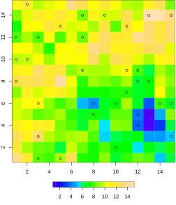
As an example, consider the simulated image in Figure 4, the circles represent the locations where we have

missing values. The processZ of interest is not observed at those locations. Our filter functiong would be

zero at those locations and 1 everywhere else.

We propose the following estimate of the spectral density of Z,

˜ IZ(ω) =

1 H₂(0)|

N

i=1

(Y(xi)−g(xi) ˜Z) exp{−iωxi}|2

whereHj(λ) = 2π

N

i=1gj(xi)eiλ T_x

i_{, thenH2(0) = 2π}N

i=1g(xi)2, and

˜ Z=

_N

i=1

Y(xi)

/

_N

i=1

g(xi)

.

Ifg(xi) = 1 for allxiinPN, thenY ≡Z on the lattice, and ˜IN reduces to the standard definition of the

2 4 6 8 10 12 14

2

4

6

8

10

12

14

2 4 6 8 10 12 14

Let us study the asymptotic properties of this estimate offZ, asN → ∞(increasing domain asymptotics).

The expected value of ˜IZ is:

E[ ˜IZ(ω)] =

π

−π

π

−πfZ(ω−φ)|H1(φ)|

2_{dφ. (11)}

Thus,E[ ˜IZ(ω)] is a weighted integral offZ(ω). Asymptotically,

E[ ˜IZ(ω)] =fZ(ω) +O(N−1). (12)

This result is obtained by using (3.12) in Brillinger (1970), since ˜IZ(ω) is the periodogram of a tapered

version ofZ.

Sharp changes in g make its Fourier transform and the squared modulus of its Fourier transform

ex-hibit side lobes. Therefore a lot of scatter missing values create very large side lobes in (11), and even if

asymptotically the bias is negligible by (12), for small samples this bias could have some impact.

We obtain now the asymptotic variance for ˜IZ,

var{I˜Z(ω)}=|H2(0)|−2H2(0)2+H2(2ω)2fZ(ω)2+O(N−1). (13)

This can be proven by applying Theorem 5.2.8 in Brillinger (1981) to ˜IZ(ω).

The quantity multiplying fZ in the expression (13) for the asymptotic variance is greater than 1 when

we have missing values, and it is 1 when there is no missing values. Thus, a large number of missing values

would increase the variance of the estimated spectrum.

We use now the estimated spectrum ˜IZ to approximate the likelihood of the spatial process Z. By

proposition 1 in Guyon (1982) we have that our estimated likelihood,

LZ =

N (2π)2

j∈JN

logfZ(2πj/n) + ˜IZ(2πj/n) (fZ(2πj/n))−1

,

(asN → ∞) converges to the exact likelihood ofZ

LZ =

1

2log|ΣN|+Z

T_Σ−1 N Z,

we have

EPθ sup

k=0,1,2supθ |L (k)

Z − L( k)

Z |=O(max(n1, n2)). (14)

3.1

Simulation study

We simulate a spatial lattice (15× 15), with 15% missing values. The location of the missing values are

represented by circles in Figure 4. The simulated process of interest is a stationary Gaussian spatial process

with an exponential covariance functionC,

C(h) =σe−|h|/ρ

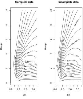
the sill parameter (σ) is 2, and the range (ρ) 3. We calculate ˜IZ, and obtain the approximated likelihood

function. Figure 5 shows a contour-plot for the likelihood function of the range and sill parameters using

the spectral approach introduced here (filling up with zeros the missing values). Figure 5 compares the full

spectral likelihood for the complete lattice (without missing values) to the approximated likelihood for the

incomplete lattice using the approach presented here. With the filling-up approach we tend to be a little

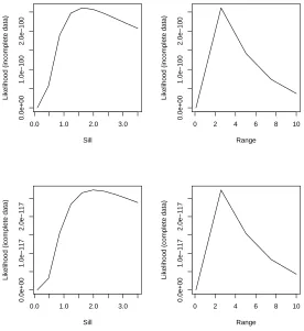
bit over-optimistic for the sill parameter, this is more clear in the next Figure, (Figure 6), in which we see

a faster decay of the likelihood function as we move away from the pseudo-MLE for the sill. But, overall

the estimated pseudo-MLEs for the sill and range, are practically the same for the incomplete and complete

datasets and right on target (Figures 5 and 6). With datasets that had more than 20% missing values these

results this did not hold any longer.

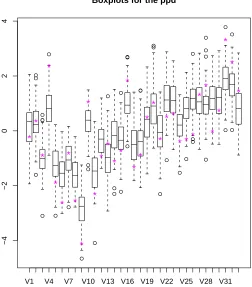
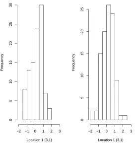
We also study the impact of this approximation on the Bayesian inference made about the data. Figure

7 shows the predictive posterior distributions (ppd) at the locations where we have missing values, using the

approach presented here to approximate the likelihood. The prior for the range is a uniform on the interval

[0,20], and the prior for the sill is

P(σ2)∝1/σ2.

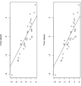
The true value is represented in Figure 7 by a star. The approximated likelihood method does not seem

to have an impact on the estimated center of the ppd (this is more clear in Figures 8 and 9). However,

as we can appreciate in Figure 8, our method seems to underestimate slightly the spread of the ppd. The

obtained ppd based on the approximated likelihood method introduced here has variance of .50 at location

(row=3,column=1) in our image, while the variance of the ppd based on the exact likelihood function is

Complete data

Sill

Range

0.0 1.0 2.0 3.0

02468

1

0

Incomplete data

Sill

Range

0.0 1.0 2.0 3.0

02468

1

0

Figure 5: Contour plot for the likelihood. Left: using the complete dataset and the Whittle approximation. Right:

using the approach presented here for incomplete datasets (with 15% missing values). Truth: Range is 3, Sill is 2.

the circles, versus the mean of the ppd using the exact likelihood and using the approximated likelihood for

incomplete lattices introduced here. We can not appreciate a difference in the center (mean) of the ppd.

4

Likelihood for irregularly spaced data

Assume Z is a continuous Gaussian spatial process of interest, observed at M irregularly spaced locations,

andfZ is the stationary spectral density ofZ. We define a processY at locationxas the integral of Z in a

block of area ∆2 centered atx,

Y(x) = ∆−2

0.0 1.0 2.0 3.0

0.0e+00

1.0e−100

2.0e−100

Sill

Likelihood (incomplete data)

0 2 4 6 8 10

0.0e+00

1.0e−100

2.0e−100

Range

Likelihood (incomplete data)

0.0 1.0 2.0 3.0

0.0e+00

1.0e−117

2.0e−117

Sill

Likelihood (icomplete data)

0 2 4 6 8 10

0.0e+00

1.0e−117

2.0e−117

Range

Likelihood (complete data)

Figure 6: Profile likelihoods using Whittle approximation for the complete dataset on a regular lattice (bottom row)

V1 V4 V7 V10 V13 V16 V19 V22 V25 V28 V31

−4

−2

0

2

4

Boxplots for the ppd

* *

* *

*

* *

*

* *

* *

*

* *

*

* *

* *

* * *

* ** **

* *

*

*

*

Figure 7: Boxplots for the predictive posterior distribution at the locations where we have missing data. The star

PPD using approx. likelihood

Location 1 (3,1)

Frequency

−2 −1 0 1 2 3

0

5

10

15

20

25

30

PPD using true likelihood

Location 1 (3,1)

Frequency

−2 −1 0 1 2 3

0

5

10

15

20

25

Figure 8: Predictive posterior distribution at location (3,1) for the irregular dataset with 15% missing values. Left:

Using the approach presented here (mean:0.19, var:0.5, we are overoptimistic). Right: Using the exact likelihood

−3 −2 −1 0 1 2

−4

−2

0

2

Mean of ppd (approximated likelihood)

True values

−3 −2 −1 0 1 2

−4

−2

0

2

Mean of ppd (true likelihood)

True values

Figure 9: True values versus the mean of the predictive posterior distribution. Left: using the approximated

where foru= (u₁, u₂) we have,

h(u) =

⎧ ⎪ ⎪ ⎨ ⎪ ⎪ ⎩

1 if|u₁|<∆/2,|u₂|<∆/2

0 otherwise.

Then, Y is also a stationary process with spectral densityfY given by:

fY(ω) = ∆−2|Γ(ω)|2fZ(ω),

whereω= (ω₁, ω₂) and Γ(ω) =h(u)e−iωu_{= [2sin(∆ω1/2)/ω1][2sin(∆ω2/2)/ω2].} For small values of ∆, fY(ω) is approximatelyfZ(ω),since we have:

lim ∆→0∆

−2_|Γ(ω)|2_{= 1.}

By (15),Y(x) can be treated as a continuous spatial process defined for allx∈D. But, here we consider the processY only on a lattice (n₁×n₂) of sample sizeN =n₁n₂, i.e. the values of xin (15) are the centroids of theN grid cells in the lattice, having spacing ∆ between neighboring sites (see Figure 10). Then, we have

that the spectral density of the lattice processY is,

f_∆,Y(ω) =

Q∈Z2

|Γ(ω+ 2πQ/∆)|2fZ(ω+ 2πQ/∆). (16)

In practice, we truncate the sum in (16) after 2N terms, we include in the Appendix (A.1) the justification.

The idea is to apply Whittle likelihood to f_∆,Y, written in terms of fZ. Therefore, we can obtain the

MLE for the covariance/spectral density parameters ofZby writing the likelihood of the processY. It might

help the reader to interpret this key idea in the spatial domain rather than the spectral domain.

• Basic idea: interpretation in the spatial domain.

The covariance for the block averages (the lattice processY) is defined as

cov(Y(xj1), Y(xj2)) =

∆−4

Bj1

Bj2

cov(Z(u), Z(v))dudv=

∆−4

Bj1

Bj2

* * * * * * * * * * * * * * * * * * * * * * * * * * * * * * * * * * * * * * * * * * * * * * * * * * * * * * * * * * * * * * * * * * * * * * * * * * * * * * * * * * * * * * * * * * * * * * * * * * * * * * * * * * * * * * * * * * * * * * * * * * * * * * * * * * * * * * * * * * * * * * * * * * * * * * * * * * * * * * * * * * * * * * * * * * * * * * * * * * * * * * * * * * * * * * * * * * * * * * * * * * * * * * * * * * * * * * * * * * * * * * * * * * * * * * * * * * * * * * * * * * * * * * * * * * * * * * * * * * * * * * * * * * * * * * * * * * * * * * * * * * * * * * * * * * * * * * * * * * * * * * * * * * * * * * * * * * * * * * * * * * * * * * * * * * * * * * * * * * * * * * * * * * * * * * * * * * * * * * * * * * * * * * * * * * * * * * * * * * * * * * * * * * * * * * * * * * * * * * * * * * * * * * * * * * * * * * * * * * * * * * * * * * * * * * * * * * * * * * * * * * * * * * * * * * * * * * * * * * * * * * * * * * * * * * * * * * * * * * * * * * * * * * * * * * * * * * * * * * * * * * * * * * * * * * * * * * * * * * * * * * * * * * * * * * * * * * * * * * * * * * * * * * * * * * * * * * * * * * * * * * * * * * * * * * * * * * * * * * * * * * * * * * * * * * * * * * * * * * * * * * * * * * * * * * * * * * * * * * * * * * * * * * * * * * * * * * * * * * * * * * * * * * * * * * * * * * * * * * * * * * * * * * * * * * * * * * * * * * * * * * * * * * * * * * * * * * * * * * * * * * * * * * * * * * * * * * * * * * * * * * * * * * * * * * * * * * * * * * * * * * * * * * * * * * * * * * * * * * * * * * * * * * * * * * * * * * * * * * * * * * * * * * * * * * * * * * * * * * * * * * * * * * * * * * * * * * * * * * * * * * * * * * * * * * * * * * * * * * * * * * * * * * * * * * * * * * * * * * * * * * * * * * * * * * * * * * * * * * * * * * * * * * * * * * * * * * * * * * * * * * * * * * * * * * * * * * * * * * * * * * * * * * * * * * * * * * * * * * * * * * * * * * * * * * * * * * * * * * * * * * * * * * * * * * * * * * * * * * * * * * * * * * * * * * * * * * * * * * * *

Figure 10: Simulation: Irregularly spaced observations. We grid the observations in a 10×10 grid, with an average

of 10 observations per grid.

where C_θ(u−v) is the covariance for the continuous underlying processZ, andθ are the covariance parameters. The continuous processZ is defined in terms of a pointwise covarianceCθ(h), but we then use the previous expression to derive the covariances of the block averagesY(xi), i= 1, . . . , N,in terms of the pointwise covarianceC_θThis is then used to define a likelihood function for the parameters of the

covariance function for the processZ in terms of the likelihood function ofY(x1), Y(x2), . . . , Y(xN).

To calculate the likelihood of Y, we first need to estimate f_∆,Y. With that purpose in mind we define

YN as,

YN(x) = 1/nx

si∈Jx

h(si−x)Z(si), (17)

where forx= (x1, x2),

J_x={s= (s₁, s₂),|x₁−s₁|<∆/2,|x₂−s₂|<∆/2}, (18)

and the cardinal of this set is|J_x|=n_x. For locationsx,such thatn_x= 0,the value ofYN(x) is not known.

As the observations become more dense, the covariance of YN converges to the covariance of Y, see

Appendix (A.1). However, the approximation ofYN toY works worse in grid cells with very few observations.

g₁(x) = n_x/n, with n the mean of the n_x values. This g₁ function plays a similar role to the g weight function (10) in the incomplete grid scenario.

We defineIg1YN(ω) the periodogram for the tappered processg1(x)YN(x),

Ig1YN(ω) =|H2∗(0)|−1

n1

s1=1 n2

s2=1

g₁(s)YN(s) exp{−isTω}

2

, (19)

whereH_k∗(λ) = 2πN_j=1gk

1(xj)eiλ

T_x j_.

The peridogramIg1YN(ω) is an asymptotically unbiased estimate off∆,Y. The bias is of orderO(N−1) +

O(¯n−1), where ¯nis the average of then2_xvalues (¯n=N_j=1n2_xj/N):

E[Ig1YN(ω)] =f∆,Y(ω) +O(N

−1_{) +O(¯n}−1_),

the proof of this result is included in the Appendix (Theorem 1).

Thus, as long as O(N/¯n)≤O(1) we have that (see Appendix, Theorem 2)

LY =

N (2π)2

j∈JN

logf∆,Y (2πj/n) +Ig1YN(2πj/n) (f∆,Y (2πj/n))

−1_{, (20)}

converges toLY = 1₂log|ΣN|+YTΣ−N1Y (exact likelihood forY), the order of convergence (in the sense of

(14)) isN1/2_.

IfM is the total number of observations of the processZ, the calculation ofLY requiresO(N log2N+M)

operations rather thanO(M3) for the exact likelihood of Z. We chooseN ≤M2/3 _{(with the equality only}

when there are not many empty cells) to satisfyO(N/¯n)≤O(1). If we haveN=M2/3_{,then the number of}

operations to obtain the likelihood function is O(M2/3_log

2M).

4.1

Simulation

We simulate 1000 observations of a Gaussian spatial process with a stationary exponential covariance

(range=.25 and sill =1). We grid the observations in a 10× 10 lattice, and we obtain an average of 10

observations per grid. Figure 10 shows the grid and Figure 11 the empirical semivariogram for the gridded

process and for the original data. The gridded process clearly shows a smaller sill (less variance) and larger

range. We want to emphasize the fact that in our approach we do not estimate the parameters of the block

covariance for the gridded process, what we do is to write this block covariance (or the corresponding

0.0 0.2 0.4 0.6

0.0

0.2

0.4

0.6

0.8

1.0

distance

semivariance

Empirical semivariogram for gridded data

0.0 0.2 0.4 0.6

0.0

0.2

0.4

0.6

0.8

1.0

distance

semivariance

Empirical semivariogram for original data

Figure 11: Empirical semivariogram for original data and gridded data. Truth: Exponential covariance, nugget=0,

range =.25, sill =1.

parameters of the point-covariance of Z. Figure 12 shows the true semivariogram forZ and the empirical

semivariogram with a confidence envelope, obtained simulating 1000 versions of the processZ, the upper and

lower limits (dashed-lines) show the maximum and minimum values of the empirical semivariograms for the

1000 simulated Gaussian processes with an exponential covariance (range=.25 and sill=1). The variogram

with the true MLE parameters (green line) is showed practically on top of the true variogram. Our approach

gives the red dotted-line in Figure 12, just slightly below the true semivariogram.

4.2

Modified version of the approximated likelihood function

The approach presented in this Section for irregularly spaced datasets performs well when there is no nugget

effect (measurement error). But, we could improve the estimation of the nugget and also the smoothness

parameter (that explains the degree of differentiability ofZ, see Stein (1999)) by adding to the likelihood

function ofY information about the behavior of the processZ(si) within grid cells.

Thus, we randomly choosemblocks (no more than 10%-15% of the blocks) and treat them as ifn_xi = 0

(i.e. we give them weight zero). We do not use the information from thesemblocks inLY, the log-likelihood

forY.

0.0 0.2 0.4 0.6 0.8

0.0

0.5

1.0

1.5

2.0

distance

semivariance

Figure 12: True semivariogram (solid line in blue, sill 1 and range .25) with an envelope, exact MLE (green line).

Estimated MLE with our spectral method (red dotted-line).

as independent):

LY + m

j=1 1

2log|Σj|+Z

T

jΣ−j1Zj, (21)

where Zj is a vector with the n_xj observations within block j, and Σj is the covariance within the block

written in terms ofC_θ(h) (covariance ofZ). The calculation of (21) is very fast, since the blocks are small, approximately of orderM1/3_.

4.3

Simulation

We simulate 1000 observations of a Gaussian spatial process with a stationary Mat´ern covariance (nugget=

.25, range=.25, smoothness parameter =3, and partial sill =1):

C(h) =σ₀I(h) + σ1 2ν−1Γ(ν)(2ν

1/2_|

h|/ρ)νKν(2ν1/2|h|/ρ), (22)

where Kνs is a modified Bessel function and θ = (σ0, ν, σ1, ρ). I(h) is an indicator function, it takes the

value 1 when h= (0,0), and it is zero otherwise. The nugget parameter is σ₀ (microscale variation). The parameterρmeasures how the correlation decays with distance; generally this parameter is called therange.

degree of smoothness of the processZ. The higher the value ofνthe smootherZwould be; e.g. whenν =1₂,

we get the exponential covariance function. In the limit asν→ ∞we get the Gaussian covariance.

We grid the observations in a 10×10 lattice (as in Figure 10). Figure 13 presents the empirical

semivar-iogram for the gridded process and for the original data. The gridded process clearly does not capture the

microscale variation, and estimates the nugget as zero. This still remains a problem when we write this block

covariance (or the corresponding spectrum) in terms of the point-covariance parameters of the continuous

underlying processZ.

The following results show the improvement in the nugget estimation by adding to the likelihood of

the gridded process,LY in (20), the information within blocks (using 10 blocks, randomly selected) using

expression (21). In Table 1, the nugget is estimated as 0, using the gridded process, and it is estimated as .3

(with standard error .23) using expression (21). Regarding the smoothness parameter, which is always very

difficult to estimate, the exact MLE is .7. We estimate this parameter as 5 using the information within 10

blocks. We should note that the spectral likelihood method for the gridded process (LY) seems to estimate

well the range and partial sill parameters and also their standard errors (s.e.). The standard errors are

obtained using expression (9). The s.e. for the range and smoothness parameters are underestimated using

LY, but when we add the information in 10% of the blocks we estimate better not only these parameters

but also the uncertainty about them.

Parameters: Nugget Partial Sill Range Smoothness

TRUTH .25 1 .25 3

MLE (exact likelihood) .24 (.2) .9 (.2) .5 (.25) .7 (3.5)

MLE (Spectral gridded) 0 (.1) .8 (.2) .12 (.2) 1 (2.1)

MLE (Spectral combining) .3 (.23) .8 (.27) .4 (.3) 5 (4.8)

Table 1. Estimated covariance parameters, the values in parenthesis are standard errors.

In the next Section we introduce a new data taper. Tappering does not help to improve the asymptotic

order of approximation of the spectral likelihood to the exact likelihood. But, it does help to obtain better

pseudo-MLE parameters, by reducing the bias in the empirical covariance and periodogram due to the edge

0.0 0.2 0.4 0.6 0.8

0.0

0.5

1.0

1.5

distance

semivariance

Variogram for gridded data

0.2 0.4 0.6 0.8 1.0 1.2

0.0

0.5

1.0

1.5

distances

variogram

Variogram for original data

Figure 13: Empirical semivariogram. Truth: Matern covariance, smoothness=3, range=.25, partial sill=1,

nugget=.25

5

New data taper

The periodogram,IN, defined in (5) in terms of the processZ, it is also the discrete Fourier transform of the

biased estimate of the covariance, the sample covariancecN(k) =N−1

(Z_s−Z)(Z¯ _s+k−Z) where¯ N is the

total number of observations and ¯Z the sample mean, rather than the unbiased version (Guyon, 1982). No

matter how largeN becomes, the periodogram always involves the tailof the sample covariance, which is a

poor estimate of the corresponding theoretical covariance, since in this region the sample covariance is based

on just a small number of pairs of observations. One of the advantages of tapering is the reduction of the bias

due to the boundary effect on the sample covariance. Edge effects are a serious problem in spatial statistics

because the number of boundary points increases with the dimension. Thus, we generally need more tapering

for the corner observations. A rounded taper gives more tapering to the corner observations, so with less

overall tapering, we get the amount of smoothing that we need without losing so much information.

We propose here a ”rounded taper”. First, we introduce some notation and we define new coordinates

(r₁, r₂)∈−n1 2,n21

×−n2

2 ,n22

in terms of (s₁, s₂)∈[0, n₁]×[0, n₂],

r₂=|s₂−(n₂−1)/2|,

d=

[r₁−(n₁/2−)]2+ [r₂−(n₂/2−)]2,

S={(r₁, r₂), s.t. r₁>(n₁/2−) and r₂>(n₂/2−)}.

We give now a partition of the grid in terms of the new coordinates (r₁, r₂)∈−n1 2,n21

×−n2

2 ,n22

(see

Figure 3), because centering the observations in this way makes it easier to define the rounded taper,

A={(r₁, r₂), s.t. r₁≤n₁/2− and r₂> n₂/2−δ}

B ={(r₁, r₂), s.t. r₂≤n₂/2− and r₁> n₁/2−δ}

C={(r₁, r₂), s.t. r₁≤n₁/2−δ and r₂< n₂/2−, or

r₁≤n₁/2− and r₂< n₂/2−δ}

D={(r₁, r₂), s.t. (r₁, r₂)∈S and d∈[−δ, ]}

E={(r1, r2), s.t. (r1, r2)∈S and d≥}

F ={(r1, r2), s.t. (r1, r2)∈S and d≤−δ}

Finally, we present the weight function,hR(),that defines the rounded data taper,

hR(r₁, r₂) =

⎧ ⎪ ⎪ ⎪ ⎪ ⎪ ⎪ ⎪ ⎪ ⎪ ⎪ ⎪ ⎪ ⎪ ⎪ ⎪ ⎪ ⎪ ⎪ ⎨ ⎪ ⎪ ⎪ ⎪ ⎪ ⎪ ⎪ ⎪ ⎪ ⎪ ⎪ ⎪ ⎪ ⎪ ⎪ ⎪ ⎪ ⎪ ⎩ 1 2

1−cos

π(n2/2−r2)

δ

for (r₁, r₂)∈A,

1 2

1−cos

π(n1/2−r1)

δ

for (r₁, r₂)∈B,

1 for (r₁, r₂)∈C orF,

1 2

1−cos

π(−d)

δ

for (r₁, r₂)∈D,

0 for (r₁, r₂)∈E.

(23)

The parametersδ and define the rounded data taper. The parameterδ ∈[0, n/2], with n= min(n₁, n₂),

plays the same role asmin the multiplicative taper (7), and the parameter∈[0, n/2] defines the rounded

region (see Figure 14).

Figure 3, illustrates the difference between the two data tapers. The black rectangle represents the border

of the site. The rounded data taper gives weight 1 to the observations inside the magenta curve, whereas

weight 1 only to the observations inside the blue rectangle. Therefore, we generally lose more information

with a multiplicative data taper, if we equalize the amount of tapering in the corners.

Figure 15 shows the spectral windows on a decibel scale along the vertical axis (ω₁= 0). The idea is to

select a data taper so thatW() is uniformly small at frequencies far from 0. Note that the spectral windows

corresponding to the two data tapers have significantly smaller side lobes thanW() with no taper. However,

notice that the widths of the main lobes of these spectral windows are slightly larger: we have suppressed

the side lobes in the windows at the expense of wider main lobes. The spectral window for the rounded

taper, at almost all frequencies along the vertical axis, is much smaller than the spectral window for the

multiplicative.

Figure 16 shows the spectral windows on a decibel scale along the diagonal (ω₁=ω₂). We see in Figure

15 that the rounded taper has a slightly broader main lobe. Along the diagonal the side lobes for both tapers

are much smaller than along the axes (compare Figures 15 and 16), and the differences between the two

tapers are also smaller along the diagonal. Thus, even if the side lobes are slightly larger for the rounded

data taper along the diagonal, overall the spectral window for the rounded data taper has better properties

(smaller side lobes) than the spectral window for the multiplicative taper.

In summary, tapering is an operation that replaces the spectral window of the periodogram with one

having better side lobe properties, which is a useful method for reducing the bias due to leakage in direct

spectral estimators. A useful characterization of spectral density functions, f,is in terms of theirdynamic

range,which we define by the ratio

10 log₁₀

max_ωf(ω) min_ωf(ω)

,

the dynamic range of a white noise process is 0. The bias in the periodogram for processes with high dynamic

range can be attributed to the side lobes of the spectral window. Thus, tapering is particularly important

for spectral densities with large dynamic range.

The asymptotic properties of the estimated covariance parameters (in terms of efficiency and consistency)

using Whittle’s likelihood and applying the data taper presented in this paper are the same as the ones

Rounded Taper

C

F F

F F

A

A

B B

D D

D D

E E

E E

Figure 14: Rounded taper. The weight in the regions F and C is 1, the weight in the regions E is 0, and

the weight in the regions A, B, and D is a cosine functionhR() that goes smoothly from 1 to 0. The two

parameters that define the rounded tapering are , andδ. The parameter is the radius of the circle that

Frequencies

log10(Spectral Windows)

0.0 0.5 1.0 1.5 2.0 2.5 3.0 3.5

-15

-10

-5

0

5

1.-No tapering 2.-Multiplicative taper 3.-Rounded taper

Figure 15: Spectral windows along the vertical axis. The horizontal axis shows the frequencies, while the

vertical axis shows the spectral window along the vertical axis (ω1= 0) on a decibel scale; for the periodogram

(line 1), for the periodogram applying amultiplicativedata taper (line 2), and for the periodogram applying

Frequencies

log10(Square spectral windows)

0 1 2 3 4 5

-20

-15

-10

-5

0

5

1.-No tapering

2.-Multiplicative taper

3.-Rounded taper

Figure 16: Spectral windows along the diagonal. The horizontal axis shows the frequencies, while the vertical

axis shows the spectral window along the diagonal (ω1 =ω2) on a decibel scale; for the periodogram (line

1), for the periodogram applying a multiplicativedata taper (line 2), and for the periodogram applying a

samples the rounded taper helps to reduce the bias in the periodogram of the spectral likelihood function.

6

Discussion

In this paper we introduce likelihood approximation methods for lattice data with missing values and for

irregularly spaced datasets. We use a spectral framework that offers enormous computational benefits. There

are other alternative spectral approaches for irregularly sampled processes that are more computationally

expensive:

• a spectral likelihood based on a periodogram for irregularly sampled processes obtained using

general-ized prolate spheroidal sequences (Bronez, 1988),

• the EM algorithm (Dempster, Laird, and Rubin 1977), which is a very well-known technique to find

maximum likelihood estimates in parametric models with incomplete data. In the EM algorithm, we

could first impute the values of the process at the locations in the grid where we have no data and

then calculate the complete-data likelihood using spectral methods. We would need to iterate through

these two steps.

The spectral likelihood approach presented here is attractive because of its simplicity and because is very

computationally efficient and fast compared to any other known likelihood approximation method for spatial

data that gives consistent estimates.

The weight function g introduced here to handle incomplete lattices, could have more sophisticated

structures than the one used in this paper. For instance, instead of just taking values 1 and 0,g could go

smoothly from 1 to 0 using a cosine function or a spline function to capture better the transition zones in the

areas with missing values. This can be particularly helpful when we have missing values clustered together,

e.g. clouds in AVHRR satellite data.

The new spatial data taper introduced in this paper, does not improve the asymptotic properties of the

estimated covariance/spectrum parameters, but with finite samples it helps to reduce the periodogram bias

due to the edge effect and therefore produces more reliable estimates. Any tapering technique is defined in

parameters. If the objective is spatial prediction, cross validation is often used to determine the values of

the taper parameters. The two parameters in the rounded data taper proposed here are andδ, and they

can be chosen such that they minimize the relative mean squared error (rmse) of the estimated periodogram.

The rmse is the mse of the periodogram divided by the squared of spectral density,f2.The mean and the

asymptotic variance of the periodogram for a tapered process are presented in Section 3, and can be used

to approximate the mse. We suggest using a plug-in approach and replace f with the periodogram in the

expression for the mse.

7

Appendix

A.1

Truncation of f∆,Y:

Let us assume that for large frequencies (as |ω| → ∞) the spectral density of a continuos spatial process

Z satisfies:

fZ(ω)∝ |ω|−α, withα >2. (24)

The spectral densities models generally used for continuous spatial process (i.e. Mat´ern) satisfy condition

(24). Under this condition we need to prove that the residual term in the expression forf_∆,Y given in (16),

when we truncate the sum the sum after 2N terms, is negligible compared to O(N−1), which is the bias of

our estimated function off_∆,Y (Section 4).

The spectral density of the lattice process Y,f_∆,Y(ω) forω∈[−π/∆, π/∆]2, is defined in (16) in terms

offZ. Here we study the order of the residual termR,

f_∆,Y(ω) =

Q∈NY

|Γ(ω+ 2πQ/∆)|2fZ(ω+ 2πQ/∆) +R(ω, NY) (25)

whereNY ={(q1, q2)∈Z2;−n1< q1< n1,−n2< q2< n2}.We have that, +∞

q1=n1 +∞

q2=n2

|Γ(ω+ 2π(q1, q2)/∆)|2fZ(ω+ 2π(q1, q2)/∆)≤

_+∞

π/∆+2πn1/∆

_+∞

π/∆+2πn2/∆|

ω₁|−1|ω₂|−1|ω₁2+ω₂2|−α/2dω₁dω₂=O(N−α/2).

Similarly, we have,

−∞

q1=−n1

−∞

q2=−n2

|Γ(ω+ 2π(q₁, q₂)/∆)|2fZ(ω+ 2π(q1, q2)/∆)≤

π/∆−2πn1/∆

−∞

π/∆−2πn2/∆

−∞ |ω1| −1_|ω

2|−1|ω21+ω22|−α/2dω1dω2=O(N−α/2).

(27)

Therefore, the order of convergence to zero of the residual term in (25) is faster than O(N−1),which is

the bias ofIg1YN (defined in (19)), and it is our estimate off∆,Y.

A.2 Theorem 1:

Consider a continuous weakly stationary spatial process Z observed at M locations in a domain D of

interest. We define two lattice processes Y (as in (15)) and YN (as in (17)), both written in terms of the

process Z, and defined on a latticen₁×n₂ coveringD, with spacing ∆ between neighboring observations.

We definef_∆,Y, the spectral density of the processY. We proposeIg1YN, defined in (19), as an estimate of

f_∆,Y. AsN → ∞and ¯n→ ∞, where ¯n=N1

in2xi andnxi is the number of observations of the processZ

in the grid celli, we have,

E[Ig1YN(ω)] =f∆,Y(ω) +O(N

−1_{) +O(¯n}−1_).

Proof of Theorem 1:

Ig1YN(ω) =|H ∗

2(0)|−1

n1

s1=1 n2

s2=1

g₁(s)YN(s) exp{−isTω}

2 .

First, we need to study the convergence of the second order moments ofYN to the ones of the processY

as the observations become more dense, i.e. as eachn_xi→ ∞.AssumeC_θ(h) is the stationary covariance of the processZ at a distanceh, with parametersθ. We have

cov(YN(x1), YN(x2)) =

1 nx1nx2

si∈Jx1

sj∈Jx2

C_θ(si−sj),

whereJ_xis defined in (18), and

cov(Y(x1), Y(x2)) = ∆−2 h(u−x1)h(v−x2)Cθ(u−v)dudv= ∆−2

B∆

B∆

where B_∆ = [−1₂∆,1₂∆]2. Clearly the covariance of Y is stationary. By the expressions above for the

covariance functions ofYN andY, we have that the covariance of YN between pointsx1 andx2, coverges to

cov(Y(x1), Y(x2)) asnx1 → ∞andnx2 → ∞. The order of convergence isO(n−x11n−x21).

Thus, it is straighforward to see that the order of converge of the covariance of the tapered processg₁YN

to the covariance ofg₁Y isO(n−1n−1),(naverage of the n_xi values). Then,

E[g₁(x1)YN(x1)g1(x2)YN(x2)] =E[g1(x1)Y(x1)g1(x2)Y(x2)] +O(n−1n−1),

uniformly in x1,x2. This is a uniform convergence, because C is a uniformly bounded function, since we assume that the variance ofZ is finite.

Thus, since

E[Ig1YN(ω)] =|H2∗(0)|−1

n1

s1=1 n2

s2=1

g₁(s)YN(s) exp{−isTω}

2 ,

we have,

E[Ig1YN(ω)] =E[Ig1Y(ω)] +N(ω) (28)

whereIg1Y is the periodogram of the tapered processg1Y. AsN → ∞,E[Ig1Y(ω)] in the expression above

converges uniformly tof_∆,Y(ω),

E[Ig1Y(ω)] =f∆,Y(ω) +O(N−1),

and the residual termN(ω) in expression (28) is of the following order,

N(ω)≤ |H₂∗(0)|−1

n1

s1=1 n2

s2=1

1

n2exp{−is

T_ω}

2

=O(¯n−1).

Therefore,

E[Ig1YN(ω)] =f∆,Y(ω) +O(N−1) +O(¯n−1).

A.3

Let us assume that the spectral density of the lattice process Y (as in (15)), f_∆,Y with parameters θ,

(a.1)f_∆,Y(ω) is rational with respect toeiω, without zeros or poles,

(a.2)the second derivative off_∆,Y inθ is continuous in θ.

All classical spectral density models satisfy these two conditions.

Theorem 2:

Assume the order of convergence to zero of ¯nasN→ ∞, is at leastO(N−1). This means,O(N/¯n)≤O(1).

Then, under conditions(a.1)-(a.2), we have that,

LY =

N (2π)2

j∈JN

logf_∆,Y (2πj/n) +Ig1YN(2πj/n) (f∆,Y (2πj/n))

−1_{, (29)}

converges toLY = 1₂log|ΣN|+YTΣ−N1Y (exact likelihood function for the lattice processY), and ifn1and

n₂ are of the same order, the rate of approximation (in the sense of (14)) isN1/2_.

Proof of Theorem 2:

By conditionO(N/¯n)≤O(1),the proposed peridogram function,Ig1YN, approximates the spectral

den-sity f_∆,Y with a bias of the same order (Theorem 1) than if we use Ig1Y, the periodogram of a tapered

version ofY. Then, by Proposition 1 in Guyon (1982). In which the convergence of the spectral Whittle

likelihood function for a tapered process g₁Y,to the exact likelihood ofY is proven. We obtain that (29)

holds and the order isN1/2.

Acknowledgements

This research was sponsored by a National Science Foundation grant DMS 0353029. The author would

like to thank Michael Stein, at the University of Chicago, for providing invaluable suggestions for the taper

function introduced in Section 5.

References

Besag, J.E. (1974). Spatial interaction and the statistical analysis of lattice systems (with discussion).

J. R. Statist. Soc. B36, 76-86.

Bessag, J.E. and Moran P.A.P. (1975). On the estimation and testing of spatial interaction in Gaussian

Bronez, T. P. (1988). Spectral estimation of irregularly sampled multidimensional processes by

gener-alized prolate spheroidal sequences. IEEE Transactions on Acoustics, Speech, and Signal Processing, 36, 1862-1873.

Caragea, P. (2003). Approximate Likelihoods for Spatial Processes. Ph.D. Dissertation at UNC.

http://www.stat.unc.edu/postscript/rs/caragea.pdf

Clinger, W. and Van Ness, J. W. (1976). On unequally spaced time points in time series. Ann. Statist.

4, 736-745.

Cram´er, H. and Leadbetter, M. R. (1967). Stationary and related stochastic processes. Sample function

properties and their applications. Wiley, New York.

Dahlhaus, R. and K¨usch,H. (1987), Edge effects and efficient parameter estimation for stationary random

fields. Biometrika,74877-882.

Bloomfield (2000). Fourier Analysis of Time Series. Wiley, New York.

Brillinger, D. R. (1970).The frequency analysis of relations between stationary spatial series,Proceedings

of the Twelfth Biennial Seminar of the Canadian Mathematical Congress,(ed. R. Pyke), Montreal, Canadian

Math. Congress, 39-81.

Brillinger, D. R. (1981). Time Series: Data Analysis and Theory. Expanded edition. Holden-Day, Inc,

San Francisco.

Guyon, X. (1982). Parameter estimation for a stationary process on a d-dimensional lattice. Biometrika,

69, 95–105.

Marcotte, D. (1996). Fast variogram computation with FFT.Computers and Geosciences,22, 1175-1186. Mat´ern, B. (1960). Spatial variation. Medded. Stat. Skogsforkskinst, 49, 5. Second ed. (1986), Lectures

Notes in Statistics 36, New York: Springer.

Neave, H.R. (1970). Spectral analysis of a stationary time series using initially scarce data. Biometrika,

57, 111-122.

Pardo-Iguzquiza, and Dowd (1997). AMLE3D: a computer program for the inference of spatial covariance

parameters by approximate maximum likelihood estimation. Comput. Geosci., 23, 793-805.

Ser. A,25, 383-392.

Priestley, M. B. (1981). Spectral Analysis and Time Series. Academic Press, London.

Stein, M. L. (1995). Fixed domain asymptotics for spatial periodograms. Journal of the Americal

Statistical Association,90, 1277-1288.

Stein, Chi and Welty. (2004). Approximating likelihoods for large spatial data sets. Journal of the Royal

Statistical Society, Series B.66, 275-296.

Stein, M. L. (1999). Interpolation of Spatial Data: some theory for kriging. Springer-Verlag, New York.

Vecchia (1988). Estimation and model identification for continuous spatial processes. Journal of the

Royal Statistical Society, Series B.50, 297-312.

Whittle, P. (1954). On stationary processes in the plane,Biometrika,41, 434-449.

Yaglom, A. M. (1987). Correlation theory of stationary and related random functions. Springer-Verlag,