Batch arrival Retrial G-queue and an unreliable server with delayed repair

(1)

Batch arrival Retrial G-queue and an

unreliable server with delayed repair

K. Kirupa 1 , Dr. K. Udaya Chandrika 2

Research Scholar, Department of Mathematics, Avinashilingam University, Coimbatore, Tamil Nadu, India 1

Professor, Department of Mathematics, Avinashilingam University, Coimbatore, Tamil Nadu, India 2

Abstract: Single server batch arrival retrial G-queue and an unreliable server with delayed repair are analyzed. Positive customers arrive in batches according to Poisson processes. If the server is idle, one of the positive customers in the batch enters for service while the rest join the orbit. Otherwise all the customers enter the orbit. Arrival of negative customer removes the positive customer being in service from the system and causes the server breakdown. The repair of the failed server starts after a random amount of time known as delay time. Expected system size, orbit size, availability and failure frequency of the server are derived. Stochastic decomposition law is verified. Numerical examples are presented to illustrate the influence of the parameters on several performance characteristics.

Keywords: Retrial queue, G-queue, server breakdown, delayed repair and stochastic decomposition.

I. INTRODUCTION

Queueing systems with repeated attempts are characterized by the fact that a customer finding all the servers busy upon arrival must leave the service area and repeat his request for service after some random time. Between trials, the blocked customers join a pool of unsatisfied customers called ‘orbit’. The retrial queueing system has been studied

extensively due to its wide applicability in telephone switching system, telecommunication

and computer networks. Recent works on retrial queue includes Aissani [1], Arivudainambi and Godhandaraman [2] and Artalejo and Li [3].

During the last decade, there has been an increasing interest in queueing system with negative customers. Queue with negative arrivals, called G-queue was first introduced by Gelenbe [5] with a view to modeling neural networks. Arrival of a negative customer induces positive customers to leave the system immediately. For a comprehensive analysis of queueing systems with negative arrivals, readers may refer to Gelenbe[6-8], Artalejo [4], Wu et.al [9] and Wu et.al [10]. In this paper, an unreliable batch arrival retrial G-queue with delayed repair is discussed.

II. MODEL DESCRIPTION

Consider a single server retrial queueing system with two types of independent arrivals, positive and negative. Positive

customers arrive in batches according to Poisson process with rate . The batch size Y is a random variable with

distribution function P(Y=k) =ck, k=1,2,…., and probability generating function C(z)= zk

1

k ck



 having first two

moments m1 and m2. If an arriving batch of positive customers finds the server free, one of the arrivals begins his

service and others join the orbit. The retrial time of the customers in the retrial queue is generally distributed with

distribution function A(x) with corresponding Laplace Stieltjes transform A(s)and conditional completion rate

) ) x ( A 1 ( ) x ( a ) x

(  

 . The Service time follows a general distribution with distribution function B(x), Laplace

(2)

Negative customers arrive singly according to Poisson process with rate



. The arrival of a negative customer removes the positive customer being in service from the system and makes the server breakdown. When the server fails, it stops providing service and waits for the repair to start. This waiting time of the server is known as delay time.

The Delay time follows a general distribution with distribution function D(x), Laplace Stieltjes transform D(s) , nth

factorial moments



_n and conditional completion rate (x)w(x) (1W(x)).

The repair time also follows a general distribution with distribution function R(x), Laplace Stieltjes transform R(s),

nth factorial moments



_n and conditional completion rate (x)f(x) (1F(x)). As soon as the repair of the server is

completed, the server enters the system and waits for a new customer.

III. ANALYSIS OF THE STEADY STATE DISTRIBUTION

Let N(t) denotes the number of customers in the orbit at time t and C(t) denotes the state of the server defined as

repair repair

for under waiting

busy idle

is is is is

server server server server

the the the the

if if if if

, 3

, 2

, 1

, 0

) t ( C





0

Define the steady state probabilities

I0 =

  t

lim

I0(t) In(x) =

  t

lim

In (x,t) , x ≥ 0, n≥1,

Pn (x)= __

t

lim

Pn(x,t), x≥0, n≥0, Dn(x)= __

t

lim

Dn(x,t), x ≥ 0, n≥0,

(3)

The system of equilibrium equations governing the model, using supplementary variable technique are given below:





I0 = 

  



 

0R0(x) (x)dx

0P0(x) (x)dx (1)

1 n ), x ( n I )) x ( ( ) x ( n I dx

d

 

   

 (2)

0 n ), x ( n

1

k ckPn k

) x ( n P )) x ( ( ) x ( n P dx

d

 

 

   

  

 ₍₃₎

0 n ), x ( n

1

k ckDn k

) x ( n D )) x ( ( ) x ( n D dx

d

 

 

   

   

 ₍₄₎

0 n ), x ( n

1

k ckRn k

) x ( n R )) x ( ( ) x ( n R dx

d

 

 

   

   

 ₍₅₎

The boundary conditions are

In(0) = (x) (x)dx

0 n

R dx ) x ( ) x (

0 n

P  

    

1 n

,



(6)

P0(0) = (x) (x)dx

0 1I 0 I 1

c  

  

 (7)

Pn(0) = (x)dx,n 1

0 n k 1

I n

1

k ck

dx ) x ( ) x (

0 n 1

I 0 I 1 n

c  



  

     



   

 (8)

Dn(0) = (x)dx,n 0

0Pn 

 

 (9)

Rn(0) = (x) (x)dx,n 0

0 n

D  

 

(10)

Normalization Condition is

I0 + 1

0

n 0 n 00

dx ) x ( n R dx

) x ( n D 0

n 0

dx ) x ( n P 1

n 0

dx ) x ( n

I  

  

 

    



  

 



  

 (11)

Define the following probability generating functions, for

z



1

I(x,z) =  1 n

n z ) x ( n

I _{, P(x,z) =} 

0 n

n z ) x ( n

P _,

D(x,z)= 

0 n

n z ) x ( n

D and R(x,z) = .

0 n

n z ) x ( n R

 



(15)

I(0,z) = (x,z) (x)dx P₀

0R

0P(x,z) (x)dx

    

  



 ₍₁₆₎

P(0,z) =

_



 

_



    

 

0 I dx ) z , x ( 0

I z

) z ( C

0

dx ) x ( ) z , x ( I z 1

(17)

D(0,z) = 

  

0

dx ) z , x (

P ₍₁₈₎

R(0,z) = 

 

0D(x,z) (x)dx

(19)

The solutions of equations (12) – (15) are obtained as

I (x,z) = I (0,z) exp {-λ+x}[1-A(x)] (20)

P(x,z) = P(0,z) exp { - (λ- λ+ C(z))x } [1- B(x)] (21)

D(x,z) = D(0,z) exp {-(λ+- λ+ C (z))x} [1- W(x)] (22)

R(x,z) = R(0,z) exp {-(λ+_{- λ}+

C (z))x} [1- F(x)] (23)

Using equations (21) and (23), equation (16) yields

I(0,z) = P(0,z)

B



(

g

(

z

))

+ R(0,z)

F



(

h

(

z

))

I

0







(24)

where g(z)C(z),h(z)C(z)

Using equations (20) and (24), equation (17) yields

P(0,z) =

z

) ( A )) z ( C 1 ( ) z ( C ) z , 0 ( I ) z ( C 0 I

  

 _ _  _ 

 

(25)

Substituting the expression of P(0,z) in equation (21) and using the resultant expression, equation (18) gives

D(0,z) =

)) z ( g ( z

))) z ( g ( B 1 )]( ( A )) z ( C 1 ( ) z ( C )[ z , 0 ( I ) z ( C 0

I       

  

 (26)

Substituting the expression of D(0,z) in equation (22) and using the resultant expression, equation (19) gives

R(0,z) =

)) z ( g ( z

)) z ( h ( * W ))) z ( g ( B 1 )]( ( A )) z ( C 1 ( ) z ( C )[ z , 0 ( I ) z ( C 0

I       

   

(27) Using equation (25) and (27), equation (24) yields

I(0,z)=

))] z ( h ( F )) z ( h ( * W ))) z ( g ( B 1 ( )) z ( g ( B ) z ( g )][ ( A )) z ( C 1 ( ) z ( C [ ) z ( zg

)] z ( zg ))) z ( h ( F )) z ( h ( * W ))) z ( g ( B 1 ( )) z ( g ( B ) z ( g )( z ( C [ 0 I

 

     

  

 

 

      



(5)

The partial probability generating function of orbit size when the server is idle is given by    0 dx ) z , x ( I ) z ( I ))] z ( h ( F )) z ( h ( * W ))) z ( g ( B 1 ( )) z ( g ( B ) z ( g )][ ( A )) z ( C 1 ( ) z ( C [ ) z ( zg )] z ( zg ))) z ( h ( F )) z ( h ( * W ))) z ( g ( B 1 ( )) z ( g ( B ) z ( g )( z ( C )][ ( * A 1 [ 0 I                        

 (29)

The partial probability generating function of the orbit size when the server is busy is given by

   0 dx ) z , x ( P ) z ( P ))] z ( h ( F )) z ( h ( * W ))) z ( g ( B 1 ( )) z ( g ( B ) z ( g )][ ( A )) z ( C 1 ( ) z ( C [ ) z ( zg )) z ( g ( B 1 )( ( * A ) 1 ) z ( C ( 0 I                      (30)

The partial probability generating function of the orbit size when the server is waiting for repair is given by

   0 dx ) z , x ( D ) z ( D ))] z ( h ( F )) z ( h ( * W ))) z ( g ( B 1 ( )) z ( g ( B ) z ( g )][ ( A )) z ( C 1 ( ) z ( C [ ) z ( zg )) z ( h ( * W 1 ))( z ( g ( B 1 )( ( * A 0 I                       (31)

The partial probability generating function of the orbit size when the server is under repair is given by

   0 dx ) z , x ( R ) z ( R ))] z ( h ( F )) z ( h ( * W ))) z ( g ( B 1 ( )) z ( g ( B ) z ( g )][ ( A )) z ( C 1 ( ) z ( C [ ) z ( zg )) z ( h ( * W )) z ( h ( * F 1 ))( z ( g ( B 1 )( ( * A 0 I                       (32)

IV. PERFORMANCE MEASURES

Probability that the server is idle is given by

I = I(z)

1

zlim =

_A

₍

₎

))]

(

B

1 )(

1 (

m

)

1 m

(

))[

(

A

1 (

₁ ₁ ₁ ₁

          



























(33)

Probability that the server is busy is given by

P = P(z)

1

zlim _

       )) ( B 1 ( 1 m (34)

Probability that the server is waiting for repair is given by

D = D(z)

1

zlim = m1 1(1 B ( ))

(6)

Probability that the server is under repair is given by

R = R(z)

1

zlim = m1 1(1 B ( ))

       (36)

The unknown constant I0 can be determined by using the normalization condition (11) as

I0 =

) ( A )) ( B 1 )( 1 1 1 ( 1 m )) ( A 1 m 1 m 1 (                            (37)

Probability generating function of the number of customers in the orbit is given by

Pq(z) = I0+ I(z)+P(z)+D(z)+R(z)

))] z ( h ( F )) z ( h ( * W ))) z ( g ( B 1 ( )) z ( g ( B ) z ( g )][ ( A )) z ( C 1 ( ) z ( C [ ) z ( zg ))]] z ( g ( B 1 ]( ) 1 ) z ( c ( [ ) z ( g ))] z ( g ( B z )[[ ( * A 0 I                          

 (38)

Mean number of customers in the orbit Lq under steady state condition is given by

2 ) 1 r D ( 2 1 r D 1 r N 1 r N 1 r D ) z ( q P dz d 1 zlim q L         

Where, Nr1(z) and Dr1(z) represent the numerator and denominator of Pq(z)

)

39 (

)) ( B 1 )( 2 2 ( 2 1 m 2 )) ( B 1 )( 1 1 ( 2 m ) 1 1 ( 1 2 1 m 2 2 )) ( B 1 ( 1 1 2 1 m 2 2 1 2 1 m 2 2 )] 1 1 ))( ( B 1 ( 1 m ) ( * B 1 m ))[ ( * A 1 ( 1 m 2 )) ( * A 1 ( 2 m 1 m 2 )) ( B 1 ( 2 m 1 r D )) ( B 1 )( 1 1 1 ( 1 m )) ( A 1 m 1 m 1 ( 1 r D 1 m ) ( * A 0 I 2 1 r N ) ( * A 0 I 1 r N                                                                                                                             Probability generating function of the number of customers in the system is given by

Ps(z) = I0+ I(z)+zP(z)+D(z)+R(z)

))] z ( h ( F )) z ( h ( * W ))) z ( g ( B 1 ( )) z ( g ( B ) z ( g )][ ( A )) z ( C 1 ( ) z ( C [ ) z ( zg ))]] z ( g ( B 1 ]( ) 1 ) z ( c ( z [ ) z ( g ))] z ( g ( B z )[[ ( * A 0 I                            (40)

Mean number of customers in the system Ls under steady state condition is given by

)

41 (

P

L

)

z

(

P

dz

d

lim

(7)

V. STOCHASTIC DECOMPOSITION

Theorem : The number of customers in the system under steady state (Ls) can be expressed as the sum of two

independent random variables, one of which is the total number of customers (L) in the batch arrival classical G-queue and unreliable server with delayed repair and the other is the number of customers in the orbit given that the server is idle (LI).

Proof:

The probability generating function π(z) of the system size in the classical batch arrival G-queue and

unreliable server with delayed repair is given by

π(z)

))]] z ( h ( F )) z ( h ( * W ))) z ( g ( B 1 ( )) z ( g ( B ) z ( g [ ) z ( zg [

)] 1 1 1 ))( ( * B 1 ( 1 m ))][ z ( g ( B 1 ( )) z ( g ( B 1 )( 1 ) z ( c ( z ))) z ( g ( B ) z ( g ) z ( zg [

 

       

                             

(42)

The probability generating function χ(z) of the number of customers in the orbit when the system is idle is given by

χ(z)

) 1 ( I 0 I

) z ( I 0 I

  

))} ( B 1 )( 1

( m {

))} ( A )) z ( C 1 ( ) z ( C ))]( z ( h ( F )) z ( h ( W ))) z ( g ( B 1 ( )) z ( g ( B ) z ( g [ ) z ( zg {

))] ( B 1 )( 1

( m )) ( A m m 1 ( [

* ))]] z ( h ( F )) z ( h ( W ))) z ( g ( B 1 ( )) z ( g ( B ) z ( g ( ) z ( zg [[

1 1 1

* *

1 1 1 1

1

*

  

 



 

  

  

 

  

 

 

          

 

 

  

             

   



(43)

From equation (42) and (43), we see that Ps(z) = π(z) χ(z) .

Hence, Ls = L + LI .

VI. RELIABILITY INDICES

Let A(t) be pointwise availability of the server at time ‘t’, that is the probability that the server is either serving a

customer or idle. We define the steady state availability of the server as A

 



t

). t ( A lim

Availability of the server is given by

A = 1 – D(1) - R(1) = )

1 1 ))( ( * B 1 ( 1 m

1    

Failure frequency of the server is given by

F = P(1) (1 B*( )) 1

m  

 

VII. NUMERICAL RESULTS

In this section, we give some numerical results to illustrate the effect of parameters on the performance characteristics. For numerical calculation, we assume that the distributions of service time, retrial time, delay time and repair time follow exponential with rate µ,η,θ and β.

The effect of varying arrival rate λ+ and λ- with the fixed values (µ, η, θ, β) = (20, 0.5, 6, 3) on I0-probability that the

server is idle in the empty system, Ls-Mean number of customers in the system, Lq -Mean number of customers in the

orbit, A -Availability of the server and F - Failure frequency of the server is given in Table (1). From the table, it is

(8)

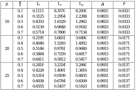
Table (2) provides I0,Ls,Lq, A and F by varying the values of µ and η for arbitrary values

(λ+_{, λ}-_{, θ, β)=(0.5, 0.5, 6,}_{3). Here, the table reveals that as µ and η increase, I}

0 increases, Ls and Lq decreases. As µ

increase, A increases and F decreases.

Table (3) shows that the effect of varying θ and β with the fixed values (λ+, λ- , µ, η)=(0.5, 0.5, 20, 0.5) on the performance measures. From this table we observe that increase in β and θ, increases I0 and A, decreases Ls and Lq

and has no effect on F.

Table 1. Performance Measures by varying λ+and λ-

λ+ λ- I0 Ls Lq A F

0.5 0.1 0.2 0.3 0.4 0.5

0.5269 0.5238 0.5207 0.5176 0.5146

0.9278 0.9403 0.9529 0.9655 0.9781

0.8930 0.9057 0.9184 0.9312 0.9440

0.9983 0.9965 0.9948 0.9931 0.9915

0.0035 0.0069 0.0103 0.0137 0.0171

0.4 0.1 0.2 0.3 0.4 0.5

0.6273 0.6251 0.6229 0.6207 0.6185

0.6127 0.6186 0.6246 0.6305 0.6364

0.5848 0.5909 0.5970 0.6031 0.6091

0.9986 0.9972 0.9959 0.9945 0.9932

0.0028 0.0055 0.0083 0.0110 0.0137

0.3 0.1 0.2 0.3 0.4 0.5

0.7249 0.7234 0.7219 0.7215 0.7190

0.3906 0.3933 0.3959 0.3985 0.4011

0.3697 0.3725 0.3752 0.3779 0.3807

0.9990 0.9979 0.9969 0.9959 0.9949

0.0021 0.0042 0.0062 0.0082 0.0102

Table 2. Performance Measures by varying µ and η

µ η I0 Ls Lq A F

10 0.3 0.4 0.5 0.6 0.7

0.1111 0.3125 0.4333 0.5139 0.5714

8.3570 2.2954 1.6329 0.9848 0.7800

8.2930 2.2288 1.2962 0.9182 0.7134

0.9833 0.9833 0.9833 0.9833 0.9833

0.0333 0.0333 0.0333 0.0333 0.0333

20 0.3 0.4 0.5 0.6 0.7

0.2195 0.4040 0.5146 0.5884 0.6411

3.6831 1.5293 0.9781 0.7259 0.5812

3.6490 1.4952 0.9440 0.6917 0.5417

0.9915 0.9915 0.9915 0.9915 0.9915

0.0171 0.0171 0.0171 0.0171 0.0171

25 0.3 0.4 0.5 0.6 0.7

0.2418 0.4228 0.5314 0.6038 0.6555

3.2334 1.4091 0.9109 0.6784 0.5437

3.2060 1.3816 0.8835 0.6509 0.5163

0.9931 0.9931 0.9931 0.9931 0.9931

0.0137 0.0137 0.0137 0.0137 0.0137

(9)

Table 3. Performance Measures by varying θ and β

β θ I0 Ls Lq A F

3 1 2 3 4 5

0.4862 0.5033 0.5089 0.5118 0.5135

1.1505 1.0368 1.0058 0.9916 0.9834

1.1163 1.0027 0.9717 0.9574 0.9493

0.9772 0.9858 0.9886 0.9900 0.9909

0.0171 0.0171 0.0171 0.0171 0.0171

4 1 2 3 4 5

0.4890 0.5061 0.5118 0.5146 0.5163

1.1320 1.0216 0.9916 0.9778 0.9699

1.0979 0.9874 0.9574 0.9437 0.9358

0.9787 0.9872 0.9900 0.9915 0.9923

0.0171 0.0171 0.0171 0.0171 0.0171

5 1 2 3 4 5

0.4907 0.5078 0.5135 0.5163 0.5180

1.1213 1.0128 0.9834 0.9699 0.9622

1.0872 0.9787 0.9493 0.9358 0.9281

0.9795 0.9880 0.9909 0.9923 0.9932

0.0171 0.0171 0.0171 0.0171 0.0171

REFERENCES

[1] Aissani, A., An MX

/G/1 Energetic Retrial Queue with Vacations and Control, IMA Journal of Management Mathematics, 22, 13-32,2011. [2] Arivudainambi, D. and Godhandaraman, P., A Batch Arrival Retrial Queue with Two Phases of Service, Feedback and K Optional Vacations, Applied Mathematical Sciences, 6(22), 1071-1087, 2012.

[3] Artalejo, J.R. and Li, Q., Performance Analysis of a Block Structured Discrete Time Retrial Queue with State Dependent Arrivals, Discrete Event Dynamic Systems, 20(3), 325-347, 2011.

[4] Artalejo, J. R., G-networks: a versatile approach for work removal in queueing networks. European Journal of Operational Research ,126 , 233-249, 2000.

[5] Gelenbe, E., Randomneural networks with negative and positive signals and product form solution. neural computation, 1, 502-510, 1989. [6] Gelenbe, E., Product-form queueing networks with negative and positive customers. Journal of applied probability,28 , 656-663, 1991. [7] Gelenbe, E., G-networks: a unifying model for neural and queueing networks. Annals of Operations Research, 48 , 433-461, 1994. [8] Gelenbe, E., The first decade of G-networks. European Journal of Operational Research, 126 , 231-232, 2000.

[9] Wu, J., Liu, Z. and Peng, Y., Analysis of the finite source MAP/PH/N retrial G-queue operating in a random environment. Applied Mathematical Modelling 35 , 1184-1193, 2011.