Truncated Life Test Sampling Plan under Log-Logistic Model

(1)

ISSN: 2319-8753

I

nternational

J

ournal of

I

nnovative

R

esearch in

S

cience,

E

ngineering and

T

echnology

(An ISO 3297: 2007 Certified Organization)

Vol. 3, Issue 7, July 2014

Copyright to IJIRSET www.ijirset.com 14397

Truncated Life Test Sampling Plan under

Log-Logistic Model

M.Gomathi1, Dr. S. Muthulakshmi2

1

Research scholar, Department of mathematics, Avinashilingam Institute for Home Science and High Education for

Women, Coimbatore, India.

2

Professorof mathematics, Department of mathematics, Avinashilingam Institute for Home Science and High

Education for Women, Coimbatore, India

ABSTRACT: Skip Lot acceptance sampling plan is proposed for the truncated life test based on product quality following log-logistic distribution. For the proposed plan the minimum sample size necessary to ensure the specified median life are obtained at the given consumer’s confidence level. The operating characteristic values are analyzed with various ratios of the true median lifetime to the specified lifetime of the product. The minimum ratios of the true population median life to the specified median life are also obtained at the specified producer’s risk. Selection and application of sampling plan is illustrated with a numerical example.

KEYWORDS: Skip-Lot acceptance sampling plan, consumer’s confidence level, producer’s risk, operating characteristic function, binomial model.

I. INTRODUCTION

Acceptance sampling plans in statistical quality control are concerned with accepting or rejecting a submitted lot on the basis of the quality of the products inspected in a sample taken from that lot. If the quality of the product is the life time of the product then acceptance sampling plan becomes a life test plan. Products or items have variations in their lifetimes even though they are produced by the same producer, same machine and under the same manufacturing conditions. Due to this variation the producer and consumer are subject to risks. Increasing the sample size may minimize both risks to certain level but this will obviously increase the cost. To reduce these risks and cost an efficient acceptance sampling scheme with truncated life test is proposed.

Several studies have been done for designing single acceptance sampling plans based on truncated life tests under various statistical distributions. With the introduction of modern quality management system such as ISO 9000, the manufacturing processes produce units of homogenous quality and provides lots of superior quality. Under this situation it is feasible and desirable to use a skip-lot procedure, where by every lot of product need not be sample inspected, and inspection of certain lots may be skipped. Under this scenario Dodge and Perry(1973)[1] introduced Skip-lot sampling plan to achieve sampling economy. This motivated to design a Skip-lot sampling plan for life test in this paper.

This paper proposes the designing of a general Skip-Lot sampling plan for time-truncated life test based on log-logistic distribution. The minimum sample sizes necessary to ensure the specified median life time at the specified consumer’s confidence level are presented in section 2 using binomial model. Operating characteristic values are analyzed in section 3. Minimum median ratios are calculated for the specified producer’s risk in section 4. In section 5 a numerical example is provided to illustrate the selection of life test plan.

II. RELATED WORK

(2)

ISSN: 2319-8753

I

nternational

J

ournal of

I

nnovative

R

esearch in

S

cience,

E

ngineering and

T

echnology

lifetime distribution, Gupta and Groll [6] for the gamma distribution, Gupta [5] designed for log-normal distribution, Kantam and Rosaiah [7] suggested for half logistic distribution and Kantam et.al. [8] for a log-logistic distribution.

III. LOG-LOGISTIC DISTRIBUTION

The lifetime variation of a product under consideration may be modelled using log-logistic distribution. The failure probability of items having a log-logistic distributed lifetime is represented through its cumulative distribution function. This attracts the applicability of log-logistic distribution to analyze the system reliability.

The probability density function and cumulative distribution function of the log logistic distribution are given respectively as







 











2

1









t

f







,

;

, t ≥ 0, σ > 0, β > 0 (1)

and









 







t

F





1 )

,

;

(

, t ≥ 0, σ > 0, β> 0 (2)

where, σ is the scale parameter and β is the shape parameter.

The median of the log-logistic distribution is derived by





1

5

0

1

5

0 















.

m

(3)

(3) shows that the median is proportional to the scale parameter, σ and independent of β.

IV. DESIGN OF THE PROPOSED SKIP LOT SAMPLING PLAN

Assume that the quality of a product can be represented by its median lifetime, m. The lot will be accepted if the submitted lot has a good quality, when the experimental data supports the null hypothesis, H0: m≥m0 against the

alternative hypothesis, H1: m<m0. where m0 is a specified median lifetime. The significance level for the test is used

through 1-P*, where P* is the consumer’s confidence level.

The designing of Skip Lot sampling plan for the truncated life test consists of obtaining (i) sample size (ii) acceptance number (iii) the ratio of true median life to the specified median life m/m0. The consumer risk, the

probability of accepting a bad lot which has the true median life below the specified life m0, is fixed as not to exceed

1-P*.

Skip-lot sampling plan is followed under the assumption that there is a continuous flow of lots from the production process and lots are offered for inspection one by one in the order of production and the production process is capable of producing units whose process quality level is stable.

The operating procedure of Skip Lot sampling plan for the truncated life test has the following steps

i. Start with normal inspection , using reference plan.(single sampling plan is used as reference plan).

(3)

ISSN: 2319-8753

I

nternational

J

ournal of

I

nnovative

R

esearch in

S

cience,

E

ngineering and

T

echnology

iii. When a lot is rejected on skipping inspection, switch to normal inspection.

iv. Screen each rejected lot and correct or replace all defective units found.

It is convenient to set the termination time as a multiple of the specified lifetime m0. Let t0= am0 where a is a

specified multiplier. Then the proposed sampling plan is characterized by five parameters (n, c ,a ,f , i ), where i is an

integer and f is a fraction.

The probability of acceptance of the lot for Skip lot sampling plan is

Pa =

_P

P

i i

) f 1 ( f

) f 1 ( fP

 

(4)

Under the binomial model C pxqn x

c 0

x x

n

P 





 (5)

Where P is the probability of acceptance of the reference plan

In this equation, p is the probability that an item fails before t0, which is given by

p =













0 0

1 t

t



=

 







 





a

m

a



0

(6)

where p at m=m0 which is given by

p =

 

 



a



1

where





1

5

0

1

5

0 















.

=1 (7)

Therefore, the minimum sample size n ensuring m≥m0 at the consumer’s confidence level

P* can be found as the solution to the following inequality

Pa≤ 1-P* (8)

There may be multiple solutions for the sample size n satisfying Equation (8). Minimization of average sample number is incorporated to find the optimal sample size for the stated specifications .

The ASN for our Skip-lot sampling plan is given by

ASN =F.ASN(R) (9)

where F is a average fraction defective and ASN(R) is the average sample number of the reference sampling plan (single sampling plan).

Determination of minimum sample size reduced to the following optimization problem

Minimize ASN =

Pi

) f 1 ( f

nf

 

(4)

ISSN: 2319-8753

I

nternational

J

ournal of

I

nnovative

R

esearch in

S

cience,

E

ngineering and

T

echnology

where n is an integer.

Minimum sample size may be obtained from (1.8) by a simple search by varying the values of n satisfying the minimum ASN . Minimum sample size are obtained for various values of consumers confidence level P* and the parameters (i ,f, a, c, β ) .

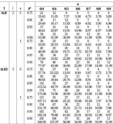
V. TABLE (1) MINIMUM SAMPLE SIZE AND ASN OF SKIP LOT SAMPLING PLAN

a

f β c P* 0.4 0.4 0.5 0.6 0.7 0.8 0.9 0.25 2 0 0.75 21

19.43 12 11.05 8 7.37 6 5.58 5 4.73 4 3.78 4 3.89

0.90 30

29.49 17 16.17 12 11.83 9 8.89 7 6.92 6 5.95 5 4.96

0.95 37

36.81 21 20.87 14 13.91 11 10.96 9 8.97 7 6.97 6 5.98 0.99 54 53.98 32 31.99 21 30.99 16 15.99 12 11.99 10 9.99 8 7.99

1 0.75 38

35.05 22 20.19 15 13.84 11 10.13 9 8.43 7 6.43 6 5.53

0.90 49

48.09 29 28.50 20 19.71 14 13.72 11 10.79 9 8.83 8 7.90

0.95 58

57.69 34 33.82 23 22.89 17 16.92 13 12.93 11 10.96 9 8.95

0.99 78

77.97 46 45.98 31 30.99 23 22.99 18 17.99 15 14.99 12 11.99

0.333 3 0 0.75 62 57.74 27 25.222 14 13.03 9 8.49 6 5.67 4 3.72 3 2.79

0.90 92

90.65 40 39.44 21 20.70 13 12.84 9 8.91 6 5.91 5 4.95

0.95 116

115.52 50 49.79 27 26.90 16 15.93 11 10.96 8 7.97 6 5.98

0.99 174

173.96 75 74.98 40 39.99 24 23.99 16 15.99 12 11.99 9 8.99

1 0.75 115

107.11 50 46.66 27 25.32 17 16.08 11 10.28 8 7.47 7 6.76

0.90 154

151.79 67 66.09 36 35.55 22 21.73 15 14.83 11 10.89 8 7.88

0.95 183

182.24 79 78.68 42 41.83 26 25.91 17 16.93 13 12.96 10 9.97

0.99 250

249.95 108 107.97 57 56.98 35 34.99 24 23.99 17 16.99 13 12.99

Table (1) show the minimum samples size for the sample when P*(= 0.75, 0.90, 0.95, 0.99), β (= 2, 3) ,i=2 ,

f=(0.25. 0.333,0.50) and a=(0.3, 0.4, 0.5, 0.6, 0.7, 0.8, 0.9) for the considered life test Skip lot sampling plans with underlying log-logistic distribution.

Numerical results in Tables (1) reveal that increase in confidence level

(5)

ISSN: 2319-8753

I

nternational

J

ournal of

I

nnovative

R

esearch in

S

cience,

E

ngineering and

T

echnology

ii. has no significant effect on sample size when the test time is relatively longer and

iii. introduces sharp growth in sample size when the shape parameter (β) increases with relatively shorter test times.

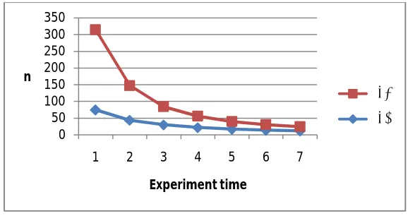
The effect of the change in the shape parameter β with reference to the minimum sample size and the

experiment time when the confidence level is at 0.95 for log-logistic distribution for the selected Skip-lot sampling test plans are given in fig.1.

Fig .1. The sample size vs. experiment time for SKSP-2 with

c=2, f=0.50 , i=2 and P*=0.95

In the above figure x-axis and y-axis denote Experiment time and sample sizes respectively, the graph shows that when the shape parameter (β) increases, the sample size rapidly increases for shorter experimental time compared to the longer experimental time.

VI. OPERATING CHARACTERISTICS (OC) VALUES

The performance of the sampling plan according to the submitted quality of the product is represented by the operating characteristics values. The probability of the acceptance will increase if the true life increases beyond the specified life. Therefore, we need to know the operating characteristic values for the proposed plan according to the ratio m/m0 of the true median life to the specified life. Obviously, a plan will be more desirable if its OC values

increase more sharply to one.

From numerical values presented in Table (2), it is seen that the OC increases to one more rapidly to move from a lower value to a higher value of the ratio m/m0. This arises due to the increase in the sample size required at

higher shape parameter. It is also seen that

i. increase in confidence level decreases the operating characteristic values for a given ratio m/m0

ii. increase in confidence level decreases the operating characteristic values for a given a

iii. increase in the ratio m/m0 increases the operating characteristic values for any given a and at any specified

confidence level.

0 50 100 150 200 250 300 350

1 2 3 4 5 6 7

n

Experiment time

β=3

(6)

ISSN: 2319-8753

I

nternational

J

ournal of

I

nnovative

R

esearch in

S

cience,

E

ngineering and

T

echnology

VII. TABLE (2) THE OC VALUES FOR SKIP LOT SAMPLING PLAN WITH β=3 , i=2

f=0.25, c=0

m/m0

P* n a 2 4 6 8 10 12

0.75 65 0.3 0.9330 0.9929 0.9979 0.9991 0.9995 0.9997

15 0.5 0.9280 0.9924 0.9978 0.9990 0.9995 0.9997

5 0.8 0.8979 0.9896 0.9970 0.9987 0.9993 0.9996

4 0.9 0.8818 0.9881 0.9965 0.9985 0.9992 0.9995

0.90 94 0.3 0.8952 0.9896 0.9970 0.9987 0.9993 0.9996

22 0.5 0.8851 0.9888 0.9967 0.9986 0.9993 0.9996

7 0.8 0.8440 0.9852 0.9957 0.9982 0.9991 0.9994

5 0.9 0.8432 0.9850 0.9957 0.9982 0.9990 0.9994

0.95 117 0.3 0.8621 0.9870 0.9962 0.9984 0.9992 0.9995

27 0.5 0.8512 0.9861 0.9960 0.9983 0.9991 0.9995

9 0.8 0.7841 0.9807 0.9945 0.9977 0.9988 0.9993

7 0.9 0.7575 0.9785 0.9939 0.9974 0.9987 0.9992

0.99 174 0.3 0.7700 0.9802 0.9944 0.9976 0.9988 0.9993

40 0.5 0.7525 0.9789 0.9940 0.9975 0.9987 0.9992

12 0.8 0.6869 0.9737 0.9926 0.9969 0.9984 0.9991

9 0.9 0.6651 0.9718 0.9921 0.9967 0.9983 0.9990

f=0.333 c=1

0.75 50 0.4 0.9783 0.9996 0.9999 0.9999 1 1

17 0.6 0.9734 0.9995 0.9999 0.9999 1 1

11 0.7 0.9733 0.9994 0.9999 0.9999 1 1

0.90 67 0.4 0.9621 0.9992 0.9999 0.9999 1 1

22 0.6 0.9561 0.9991 0.9999 0.9999 1 1

15 0.7 0.9558 0.9990 0.9999 0.9999 1 1

0.95 79 0.4 0.9481 0.9990 0.9999 0.9999 1 1

26 0.6 0.9393 0.9988 0.9998 0.9999 0.9999 1

17 0.7 0.9371 0.9987 0.9998 0.9999 0.9999 1

0.99 108 0.4 0.9057 0.9982 0.9998 0.9999 0.9999 1

35 0.6 0.8921 0.9979 0.9998 0.9999 0.9999 1

24 0.7 0.8765 0.9975 0.9997 0.9999 0.9999 1

The OC values as a function of the ratio m/m0, P*, a and β are presented in Table (2) when P* (= 0.75, 0.90,

0.95, 0.99), β = 3 ,i=2 , c=(0,1), f=(0.25. 0.333) and a=(0.3, 0.4, 0.5, 0.6, 0.7, 0.8, 0.9) , m/m0=(2,4,6,8,10,) for the

(7)

ISSN: 2319-8753

I

nternational

J

ournal of

I

nnovative

R

esearch in

S

cience,

E

ngineering and

T

echnology

VIII. MINIMUM MEDIAN RATIOS

The producer may be interested to know what will be the minimum product quality level to be maintained in

order to keep the producer’s risk at the specified level. At the specified producer’s risk of α the minimum ratio m/m0

can be obtained by solving

Pa≥ 1−α where Pa is given in (4). (10)

Numerical values in thesetables reveal that

i. increase in shape parameter β decreases the minimum median ratios at the specified consumer’s confidence

level, producer’s risk and a.

ii. increase in consumer’s confidence level increases the minimum median ratios at the specified a and producer’s risk and

iii. increase in a increases the minimum median ratios at the specified consumer’s confidence level, producer’s

risk and β.

IX.TABLE (3) MINIMUM MEDIAN RATIOS TO THE SPECIFIED LIFE AT α= 0.05 ,β=2 ,i=2

a

f c P* 0.3 0.4 0.5 0.6 0.7 0.8 0.9

0.25 0 0.75 3.324 3.345 3.408 3.536 3.760 3.835 4.315

0.90 3.975 3.986 4.181 4.340 4.460 4.714 4.834

0.95 4.416 4.432 4.519 4.802 5.064 5.097 5.303

0.99 5.337 5.475 5.540 5.799 5.854 6.103 6.134

1 _0.75 _2.182 _2.195 _2.245 _2.280 _2.383 _2.550 _2.659

0.90 2.484 2.532 2.611 2.495 2.660 2.723 2.868

0.95 2.706 2.748 2.808 2.877 2.910 3.040 3.064

0.99 3.144 3.207 3.276 3.369 3.458 3.590 3.742

0.333 0 0.75 3.644 3.759 3.831 3.976 4.229 4.316 4.855

0.90 4.390 4.501 4.698 4.878 5.363 5.730 5.963

0.95 4.892 4.978 5.077 5.397 5.363 5.730 5.963

0.99 5.993 6.149 6.223 6.515 6.578 6.858 6.895

1

0.75 0.90 0.95 0.99

2.272 2.351 2.405 2.445 2.557 2.737 2.856

2.631 2.664 2.723 2.782 2.852 2.922 3.079

2.871 2.943 3.008 3.083 3.120 3.260 3.287

3.365 3.434 3.508 3.609 3.706 3.709 3.843

(8)

ISSN: 2319-8753

I

nternational

J

ournal of

I

nnovative

R

esearch in

S

cience,

E

ngineering and

T

echnology

X. SELECTION OF LIFE TEST PLANS

Example . Suppose also that the producer would like to know whether the median lifetime of the product is longer than or equal to 1000 hours at the consumer’s confidence level of 0.95. The experimenter wants to stop an experiment at 500 hours the Skip-lot sampling plan in order to reduce the cost. This leads to the experiment termination multiplier as a=0.5, β=2, f=0.25 ,c=0 ,i=2. Table (1) gives the minimum sample size to be used is n=14.This sampling plan is interpreted as follows.

Select a sample of size n=14 and put on test for 500 hours and the lot will be accepted if no failure occurs during the experiment otherwise the lot is rejected .

The probability of acceptance increases as the quality improves. The producer wants to minimize the producer’s risk when the quality improves. Therefore, the producer is interested in knowing what quality level will lead to the producer’s risk of less than 0.05. The quality in terms of the median ratio from Table (3) for α = 0.05 is 4.519.

So, the true median required of the product of lots should be at least 4519 hours.

XI.CONCLUSION

A Skip lot sampling plan for truncated life test is proposed in order to make a decision on the submitted lot under the assumption that the lifetime of the products follows a log-logistic distribution, which is useful in system reliability analysis because its pattern of failure rate is quite versatile

.

REFERENCES

[1] Dodge,H.F. and Perry,R.L.(1971) A system of Skip-Lot plans for Lot by Lot inspection, Annual Technical Conference Transaction , American Society for quality control , pp.469-477.

[2] Duncan, A.J. (1986) Quality Control and Industrial Statistics, 5th ed., Richard D. Irwin, Homewood, Illinois. [3] Epstein, B. (1954) Truncated life tests in the exponential case, Ann. Math. Statist. 25, pp. 555-564.

[4] Goode, H.P. and Kao, J.H.K. (1961) Sampling plans based on the Weibull distribution, In Proceeding of the Seventh National Symposium on

Reliability and Quality Control, Philadelphia, pp. 24-40.

[5] Gupta, S.S. (1962) Life test sampling plans for normal and lognormal distributions, Technometrics 4, pp. 151-175.

[6] Gupta, S.S. and Groll, P.A. (1961) Gamma distribution in acceptance sampling based on life tests, J.Am. Statist. Assoc. 56, pp. 942-970. [7] Kandam, R.R.L., Rosaiah, K. and Srinivasa Rao, G. (2001) Acceptance sampling based on life tests: log-logistic model, Journal of Applied

Statistics, 28(1), pp. 121-128.