ABSTRACT
SHIH, ROBERT. Stochastic Target Problem With Jump Diffusion. (Under the direction of Negash Medhin.)
This dissertation deals with Stochastic Target Problem. The target problem is a new class of stochastic control problem. In finance, it is closely related to option pricing and hedging problem in a high-frequency trading market. We study the minimal initial capital needed in order to super-replicate a given contingent claim at a specified maturity time.
A Levy process is introduced to describe the dynamics of the state process and two different ways to solve the target problem are given in this work. In the first method we use dynamic programming to derive an integro-differential equation to characterize the solution. In the second method, we make perturbations on the optimal control to get a maximum principle which consists of a system of forward-backward stochastic differential equations.
A classical way to model the stock price process is using a linear stochastic differential equation with an assumption that the investor is ”small”, which means his/her trading strategy and financial status cannot affect the stock price. Therefore, in a classical model of stock price process, the coefficient of the process is independent of the wealth process and the trading strategy of the investor. However, in recent years, some people have started discussing the behavior of ”large investor” models in which the stock price can be affected by the investor’s financial status and trading strategy. Furthermore, the dynamics of stock prices becomes non-linear.
Stochastic Target Problem With Jump Diffusion
by Robert Shih
A dissertation submitted to the Graduate Faculty of North Carolina State University
in partial fulfillment of the requirements for the Degree of
Doctor of Philosophy
Operations Research
Raleigh, North Carolina 2012
APPROVED BY:
Thom J. Hodgson Tao Pang
Min Kang Negash Medhin
DEDICATION
BIOGRAPHY
ACKNOWLEDGEMENTS
TABLE OF CONTENTS
List of Figures . . . vii
Chapter 1 Deterministic control . . . 1
1.1 Introduction . . . 1
1.2 Deterministic control problem . . . 1
1.3 Necessary conditions for deterministic problem . . . 2
1.4 Conclusion . . . 12
Chapter 2 Stochastic control . . . 13
2.1 Introduction . . . 13
2.2 Stochastic control problem . . . 13
2.3 Necessary conditions for stochastic problem . . . 14
2.4 Conclusion . . . 31
Chapter 3 Stochastic control with jump diffusion. . . 32
3.1 Introduction . . . 32
3.2 Jump diffusion in high-frequency trading market . . . 32
3.3 Stochastic control problem with jump diffusion . . . 40
3.4 Necessary conditions for jump diffusion problem . . . 42
3.5 Relation to dynamic programming . . . 64
3.6 Sufficient condition for jump diffusion problem . . . 73
3.7 Conclusion . . . 76
Chapter 4 Target problem . . . 77
4.1 Introduction . . . 77
4.2 An example: superreplication problem in finance . . . 78
4.3 1-dimensional stochastic target problem with jump diffusion . . . 82
4.4 When the optimal trajectory hits the boundary of the target at maturity time T 84 4.5 When the optimal trajectory does not hit the boundary of the target at maturity timeT . . . 93
4.6 n-dimensional stochastic target problem with jump diffusion . . . 96
4.7 Conclusion . . . 98
Chapter 5 Application in finance . . . 99
5.1 Introduction . . . 99
5.2 Stock price process . . . 100
5.3 The model . . . 106
5.4 Model parameter estimation . . . 109
Chapter 6 Numerical methods and results . . . .116
6.1 Introduction . . . 116
6.2 Function approximation . . . 119
6.3 Dynamic programming without jump . . . 122
6.4 Dynamic programming with jump . . . 130
6.5 Numerical result . . . 137
6.6 Conclusion . . . 140
LIST OF FIGURES
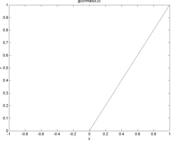
Figure 4.1 The penalty function g . . . 84
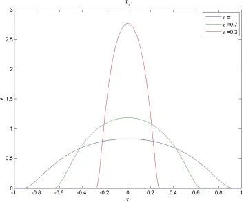
Figure 4.2 The graph of function φ . . . 86
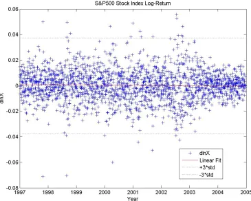
Figure 5.1 S&P stock index log-return . . . 110
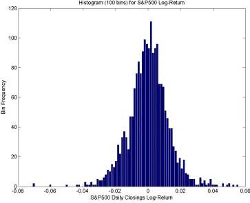
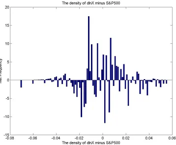
Figure 5.2 Sample histogram of S&P500 log-return . . . 111
Figure 5.3 Theoretical histogram of S&P500 log-return . . . 114
Figure 5.4 Error plot . . . 115
Figure 6.1 Cubic Spline Basic functions . . . 121
Figure 6.2 Linear Spline Basic functions . . . 122
Figure 6.3 Value function Φ(t, y) of (P2) by cubic spline family . . . 138
Figure 6.4 Optimal control by cubic spline family . . . 139
Figure 6.5 Value function Φ(t, y) of (P2) by linear spline family . . . 140
Chapter 1
Deterministic control
1.1
Introduction
In this chapter, we use perturbation method to derive maximum principle for a deterministic continuous-time control problem. Maximum principle is a set of necessary conditions character-izing optimal control and trajectory. We follow Bensoussan [5] in deriving maximum principle.
1.2
Deterministic control problem
We suppose that
f(t, x, u) : [0, T]×Rn×Rk→R
b(t, x, u) : [0, T]×Rn×Rk→Rn
g(x) : Rn→R
are continuous differentiable functions, and satisfy the usual conditions that we need to guar-antee the existence of solution of the following deterministic control problem.
minimize J(u(.)) = Z T
0
The system of differential equation in (P1) is called the state equation. The vector x which belongs to Rn is called the state variable, and the functionx(t) inH1(0, T,Rn) which satisfies the state equation will be called the trajectory corresponding tou(t), andx0is a given vector in
Rn. On the other hand, the vectoru is called the control variable, and the non-empty, closed, convex setKis the control constraint. We suppose that the state equation has one and only one solution when u(t) is given. Denote the optimal control-solution pair for (P1) is (u∗(t), x∗(t)).
A pair of functions (x(t), u(t)) is called an admissible pair if u(t) is an admissible control corresponding to trajectoryx(t). We suppose the optimal solution of problem(1) always exists, and denote the optimal solution pair by (x∗(t), u∗(t)). That is, we can always find (x∗(t), u∗(t)), such that
J(u∗(.))≤J(u(.))
for all admissible pairs (x(t),u(t)). Our objective is to look for a set of necessary conditions to characterize u∗(t) and x∗(t) in the following sections.
1.3
Necessary conditions for deterministic problem
For simplicity, we will sometimes ignore the arguments and use x∗ orxto denote the function x∗(t) or x(t). We will also use u∗ or uto denote the functionu∗(t) or u(t).
We begin with the necessary conditions. First of all, we make perturbations on the optimal controlu∗. Let
uθ =u∗+θv
where v = v(t) is an admissible control. According to our assumptions in Section 2, we can find one and only onexθ which is the trajectory corresponding touθ. That is
dxθ = b(t, xθ(t), uθ(t))dt
xθ(0) = x0
xθ(t)−x∗(t) = x0+
Z t
0
b(s, xθ(s), uθ(s))ds
−x0−
Z t
0
b(s, x∗(s), u∗(s))ds =
Z t
0
b(s, xθ, uθ)−b(s, x∗, u∗)ds
= Z t
0
Z 1
0
{bx(s, x∗+λ(xθ−x∗), u∗+λ(uθ−u∗))(xθ−x∗)
+bu(s, x∗+λ(xθ−x∗), u∗+λ(uθ−u∗))(uθ−u∗)}dλ ds
Then, we have
xθ(t)−x∗(t)
θ =
Z t
0
Z 1
0
{bx(s, x∗+λ(xθ−x∗), u∗+λ(uθ−u∗))
xθ−x∗
θ +bu(s, x∗+λ(xθ−x∗), u∗+λ(uθ−u∗))v}dλ ds
wherebx and bu denote the partial derivative ofb with respect tox and u, etc..
The following Lemma is used to determine the limit of xθ(t)−x
∗(t)
θ as θtends to zero.
Lemma 1.3.1. We define a functionZ(t)inH1(0, T,Rn) by the system of differential equation
dZ = {bx(t, x∗(t), u∗(t))Z(t) +bu(t, x∗(t), u∗(t))v(t)}dt
Z(0) = 0
Then, xθ(t)−x
∗(t)
θ −→ Z(t) in L
Consider the following functions
Lemma 1.3.2.
xθ(t) = x0+
Z t
0
b(s, xθ(s), uθ(s))ds
x∗(t) = x0+
Z t
0
b(s, x∗(s), u∗(s))ds Z(t) =
Z t
0
{bx(s, x∗(s), u∗(s))Z(s) +bu(s, x∗(s), u∗(s))v(s)}ds
and letyθ =
xθ−x∗
θ −Z
Then, we have
yθ =
Z t
0
b(s, xθ, uθ)−b(s, x∗, u∗)
θ
−bx(s, x∗, u∗)Z−bu(s, x∗, u∗)v ds
= Z t
0
Z 1
0
{bx(s, x∗+λ(xθ−x∗), u∗+λ(uθ−u∗))yθ
+[bx(s, x∗+λ(xθ−x∗), u∗+λ(uθ−u∗))−bx(s, x∗, u∗)]Z
+[bu(s, x∗+λ(xθ−x∗), u∗+λ(uθ−u∗))−bu(s, x∗, u∗)]v}dλ ds
Since the functions Z and v belong to L2, we can take sufficiently large number M, such that both of their 2-norms are less than or equal to M. Also assume that |bx| ≤ M. By Holder’s
|yθ|2 ≤ (
Z t
0
Z 1
0
{|bx(s, x∗+λ(xθ−x∗), u∗+λ(uθ−u∗))| |yθ|
+|bx(s, x∗+λ(xθ−x∗), u∗+λ(uθ−u∗))−bx(s, x∗, u∗)| |Z|
+|bu(s, x∗+λ(xθ−x∗), u∗+λ(uθ−u∗))−bu(s, x∗, u∗)| |v|}dλ ds)2
≤ 2( Z t
0
Z 1
0
|bx(s, x∗+λ(xθ−x∗), u∗+λ(uθ−u∗))| |yθ|dλ ds)2
+2( Z t
0
Z 1
0
|bx(s, x∗+λ(xθ−x∗), u∗+λ(uθ−u∗))−bx(s, x∗, u∗)| |Z|dλ ds)2
+2( Z t
0
Z 1
0
|bu(s, x∗+λ(xθ−x∗), u∗+λ(uθ−u∗))−bu(s, x∗, u∗)| |v|dλ ds)2
≤ 2M2 T2 Z t
0
|yθ|2 ds
+2M2 Z t
0
Z 1
0
|bx(s, x∗+λ(xθ−x∗), u∗+λ(uθ−u∗))−bx(s, x∗, u∗)|2 dλ ds
+2M2 Z t
0
Z 1
0
|bu(s, x∗+λ(xθ−x∗), u∗+λ(uθ−u∗))−bu(s, x∗, u∗)|2dλ ds
≤ 2M2 T2 Z T
0
|yθ|2ds+ 2M2ϑ(θ)
where ϑ(θ) = Z T 0 Z 1 0
|bx(s, x∗+λ(xθ−x∗), u∗+λ(uθ−u∗))−bx(s, x∗, u∗)|2 dλ ds
+ Z T
0
Z 1
0
|bu(s, x∗+λ(xθ−x∗), u∗+λ(uθ−u∗))−bu(s, x∗, u∗)|2dλ ds
and clearlyϑ(θ) tends to zero when θ tends to zero. By Gronwall’s inequality, we have
|yθ|2 ≤2M2ϑ(θ)e2M
2T2t
∀t∈[0, T]
Therefore
Z T
0
|yθ|2dt≤
Z T
0
the right hand side tends to zero when θtends to zero. So, yθ tends to zero inL2. That is,
xθ−x∗
θ −→Z in L
2
The proof is done.
Now, we are ready to consider the change in J as a result of the perturbation in the optimal controlu∗.
J(uθ)−J(u∗)
=g(xθ(T))−g(x∗(T))
+ Z T
0
f(t, xθ(t), uθ(t))−f(t, x∗(t), u∗(t))dt
= Z 1
0
gx(x∗(T) +λ(xθ(T)−x∗(T)))·(xθ(T)−x∗(T))dλ
+ Z T
0
Z 1
0
fx(t, x∗+λ(xθ−x∗), u∗+λ(uθ−u∗))·(xθ−x∗)dλ dt
+ Z T
0
Z 1
0
fu(t, x∗+λ(xθ−x∗), u∗+λ(uθ−u∗))·(uθ−u∗)dλ dt
Then we divide both sides byθ
J(uθ)−J(u∗)
θ
= Z 1
0
gx(x∗(T) +λ(xθ(T)−x∗(T)))·
xθ(T)−x∗(T)
θ dλ
+ Z T
0
Z 1
0
fx(t, x∗+λ(xθ−x∗), u∗+λ(uθ−u∗))·
xθ(t)−x∗(t)
θ dλ dt
+ Z T
0
Z 1
0
fu(t, x∗+λ(xθ−x∗), u∗+λ(uθ−u∗))·v(t)dλ dt
v.
Proposition 1.3.3. The Gateaux derivative of J along the direction v is
dJ(u∗;v) =gx(x∗(T))·Z(T) +
Z T
0
fx·Z+fu·v dt
Our next step is to define dual variables for the costate problem. Consider the equation
dζ(t) = {bx(t, x∗(t), u∗(t))ζ(t) + Φ(t)}dt
ζ(0) = 0
where Φ is a function in L2(0, T;Rn). And we suppose that for each Φ, we can find one and only one ζ inH2(0, T;Rn). Then, for each Φ, we can consider the quantity
Z T
0
fx·ζ dt+gx(x∗(T))·ζ(T)
This map is linear and bounded. By Riesz representation theorem, we can find one and only one function p(t) in L2(0, T;Rn), such that for all Φ in L2(0, T;Rn), we have
Z T
0
p(t)·Φ(t)dt= Z T
0
fx(t)·ζ(t)dt+gx(x∗(T))·ζ(T)
The p(t) will be called the dual variable or adjoint variable. On the other hand, we define the Hamiltonian
H(t, x, u, p) =f(t, x, u) +b(t, x, u)·p
Using the notation of Hamiltonian with Φ =buv and ζ =Z, we conclude
dJ(u∗;v) = Z T
0
Proposition 1.3.4. For (P1), we have the maximum principle
Hu(t, x∗(t), u∗(t), p(t))·(v−u∗(t))≥0
for all v∈K and almost everywhere t in [0,T].
Proof:
Since (u∗, x∗) is the optimal pair of problem(1), we know the Gateaux derivative of J(u(.)) at u∗(.) along the direction v(.)−u∗(.) is non-negative. That is,
Z T
0
Hu(t, x∗(t), u∗(t), p(t))·(v(t)−u∗(t))dt = dJ(u∗(.);v(.)−u∗(.))≥0
Let v be any fixed vector in K , t be a Lebesgue point in (0, T), and ε > 0 , such that (t, t+ε)∈[0, T]. Then, we consider the function
v(s) = (
v, s∈(t, t+ε) u∗(s), otherwise
Clearly the function always belongs to K. On the other hand, sinceu∗ belongs to L2, we have
Z T
0
|v·v|dt =
Z t+ε
t
|v·v|dt+ Z
[0,T]\(t,t+ε)
|u∗·u∗|dt
≤ |v·v|ε+|u∗|2 <∞
So,v(.) belongs toL2 and it is an admissible control. Then, we have Z t+ε
t
Hu(t, x∗(t), u∗(t), p(t))·(v−u∗(t))dt=
Z T
0
Hu(t, x∗(t), u∗(t), p(t))·(v(t)−u∗(t))dt≥0
Lettingε tends to 0 1
ε Z t+ε
t
Hu(t, x∗(t), u∗(t), p(t))·(v−u∗(t))dt−→Hu(t, x∗(t), u∗(t), p(t))·(v−u∗(t)) a.e.
So, we conclude that
for a.e t∈[0, T], and allv∈K The proof is done.
The next Proposition is another way to characterize the adjoint variable.
Proposition 1.3.5. p(t) is the adjoint variable we defined by Riesz representation theorem, if and only if it satisfies the costate equation
dp = −Hx(t, x∗, u∗, p)dt=−{fx(t, x∗, u∗) +bx(t, x∗, u∗)∗p}dt
p(T) = gx(x∗(T))
Where b∗x is the transpose of bx.
Proof:
Firstly, we suppose p(t) is the solution of the costate equation and proof that it satisfies the Riesz representation theorem. According to Integration by Parts, we have
d(p(t)·ζ(t)) = ζ(t)·dp(t) +p(t)·dζ(t)
= ζ(t)· {−fx(t, x∗, u∗)dt+bx(t, x∗, u∗)∗p(t)dt}
+p(t)· {bx(t, x∗, u∗)ζ(t)dt+ Φ(t)dt}
= −fx(t, x∗, u∗)·ζ(t)dt+p(t)·Φ(t)dt
Since ζ(0) = 0 andp(T) =gx(x∗(T)), we have
gx(x∗(T))·ζ(T) = p(T)·ζ(T)
= p(0)·ζ(0) + Z T
0
−fx(t, x∗, u∗)·ζ(t) +p(t)·Φ(t)dt
Z T
Then,
Z T
0
p(t)·Φ(t)dt= Z T
0
fx(t, x∗, u∗)·ζ(t)dt+gx(x∗(T))·ζ(T)
Therefore p(t) is the adjoint variable we defined by Riesz representation theorem.
Secondly, let’s suppose p(t) is given by the Riesz representation theorem, and prove that it must satisfies the costate equation. Consider the matrix equation
dΨ(t) = bx(t, x∗, u∗)Ψ(t)dt
Ψ(0) = I
where I is the identity matrix. Then Ψ(t) is the fundamental solution of the equation corre-sponding ζ(t). It can be shown that the fundamental equation has exactly one solution, that is, the Ψ(t) exists and unique [4][5]. Sinceζ(0) = 0 we have
ζ(t) = Ψ(t)ζ(0) + Ψ(t) Z t
0
Ψ−1(s)Φ(s)ds = Ψ(t)
Z t
0
Ψ−1(s)Φ(s)ds
NOTATION: Here and Chapter 2 and 3, we use −∗ as a notation of putting inverse and transpose operations on a matrix. More precisely, we define
According to integration by parts, we have Z T
0
p(t)·Φ(t)dt = Z T
0
fx(t, x∗, u∗)·ζ(t)dt+gx(x∗(T))·ζ(T)
= Z T
0
fx(t, x∗, u∗)· {Ψ(t)
Z t
0
Ψ−1(s)Φ(s)ds}dt +gx(x∗(T))· {Ψ(T)
Z T
0
Ψ−1(s)Φ(s)ds}
= Z T
0
Z t
0
fx(t, x∗, u∗)· {Ψ(t)Ψ−1(s)Φ(s)}ds+gx(x∗(T))· {Ψ(T)Ψ−1(t)Φ(t)}dt
= Z T
0
Z T
t
fx(s, x∗, u∗)· {Ψ(s)Ψ−1(t)Φ(t)}ds+gx(x∗(T))· {Ψ(T)Ψ−1(t)Φ(t)}dt
= Z T
0
Φ(t)·Ψ−∗(t){
Z T t
Ψ(s)∗fx(s, x∗, u∗)ds+ Ψ(T)∗gx(x∗(T))}dt
= Z T
0
Φ(t)·Ψ−∗(t){−
Z t
0
Ψ(s)∗gx(s, x∗, u∗)ds
+ Z T
0
Ψ(s)∗fx(s, x∗, u∗)ds+ Ψ(T)∗gx(x∗(T))}dt
for all Φ(t)∈L2. Then,
p(t) = Ψ−∗(t){−
Z t
0
Ψ(s)∗fx(s, x∗, u∗)ds+
Z T
0
Ψ(s)∗fx(s, x∗, u∗)ds+ Ψ(T)∗gx(x∗(T))}
By letting t=T, we obtain the boundary condition
p(T) = Ψ−∗(T){−
Z T
0
Ψ(s)∗gx(s, x∗, u∗)ds+
Z T
0
Ψ(s)∗gx(s, x∗, u∗)ds+ Ψ(T)∗gx(x∗(T))}
= gx(x∗(T))
Since dΨ(t)
dt =bxΨ, we have
dΨ(t)∗ dt = Ψ
∗b∗
x. From above,
Ψ(t)∗p(t) =−
Z t
Ψ(s)∗fx(s, x∗, u∗)ds+
Z T
Therefore
dΨ(t)∗
dt p(t) + Ψ(t)
∗dp(t)
dt =−Ψ(t)
∗f
x(t, x∗, u∗)
dp(t)
dt =−fx(t, x
∗, u∗)−b
x(t, x∗, u∗)∗p=−Hx(t, x∗, u∗, p)
The proof is done.
Proposition 1.3.6. Necessary Conditions for (P1)
Let (u∗,x∗) be the optimal pair for (P1), then we can find corresponding p(t) belongs toL2(0, T;Rn),
such that
dx∗ = Hp(t, x∗, u∗, p)dt=b(t, x∗, u∗)
x(0) = x0
dp = −Hx(t, x∗, u∗, p)dt=−{fx(t, x∗, u∗) +bx(t, x∗, u∗)∗p}dt
p(T) = gx(x∗(T))
Hu(t, x∗(t), u∗(t), p(t))·(v−u∗(t))≥0 ∀v∈K
1.4
Conclusion
Chapter 2
Stochastic control
2.1
Introduction
In this chapter, we use perturbation method to derive maximum principle of a stochastic control problem. Maximum principle is a set of necessary conditions characterizing optimal control and trajectory. We follow Bensoussan [5] in deriving maximum principle.
2.2
Stochastic control problem
We suppose that
f(t, x, u) : [0, T]×Rn×Rk →R
b(t, x, u) : [0, T]×Rn×Rk →Rn
σ(t, x, u) : [0, T]×Rn×
Rk →Rn×n g(x) : Rn→R
minimize J(u(.)) = E[ Z T
0
f(t, x(t), u(t))dt+g(x(T))] (P1) subject to dx = b(t, x(t), u(t))dt+σ(t, x(t), u(t))dBt
x(0) = x0
The stochastic differential equation is defined on the probability space (Ω, F, P). Bt is an n
dimensional Brownian motion and the filtration Ft which generated by Bt satisfies the usual
conditions. x(t) =xt=x(t, ω) and u(t) = ut =u(t, ω), forω ∈Ω. The stochastic differential
equation in (P1) will be called the state equation. The vector x which belongs to Rn will be called the state variable, and the function x(t) which satisfies the state equation will be called the trajectory corresponding to u(t), and x0 is a given vector in Rn. On the other hand, the vector u is called the control variable, and the non-empty, closed, convex set K is the control constraint. We suppose that the state equation has one and only one solution when u(t) is given. All the state variable and controls in this thesis are predictable process, and it can be shown that their perturbations will be also predictable[4]. Denote the optimal control-solution pair for (P1) by (u∗(t), x∗(t)). The state equation can also be written as the form
dx = b(t, x(t), u(t))dt+
n
X
j=1
σj(t, x(t), u(t))dBj
x(0) = x0
whereσj is the jth column ofσ and Bj is the jth element ofBt.
2.3
Necessary conditions for stochastic problem
For simplicity, we will sometimes ignore the arguments and use x∗ orxto denote the function x∗(t) or x(t). We will also use u∗ or uto denote the functionu∗(t) or u(t).
We begin with the necessary conditions. First of all, we make perturbations on the optimal controlu∗. Let
where v = v(t) is an admissible control. According to our assumptions in Section 2, we can find one and only onexθ which is the trajectory corresponding touθ. That is
dxθ = b(t, xθ(t), uθ(t))dt+σ(t, xθ(t), uθ(t))dBt
xθ(0) = x0
In order to discuss the change inJ corresponding to the perturbation in u∗, we need to discuss the change in the dynamics first. By mean value theorem, we have the following
xθ(t)−x∗(t) = x0+
Z t
0
b(s, xθ(s), uθ(s))ds+
Z t
0
σ(s, xθ(s), uθ(s))dBs
−x0−
Z t
0
b(s, x∗(s), u∗(s))ds+ Z t
0
σ(s, x∗(s), u∗(s))dBs
= Z t
0
b(s, xθ(s), uθ(s))−b(s, x∗(s), u∗(s))ds
+ Z t
0
σ(s, xθ(s), uθ(s))−σ(s, x∗(s), u∗(s))dBs
= Z t
0
Z 1
0
{bx(s, x∗+λ(xθ−x∗), u∗+λ(uθ−u∗))(xθ−x∗)
+bu(s, x∗+λ(xθ−x∗), u∗+λ(uθ−u∗))(uθ−u∗)}dλ ds
+
n
X
j=1
Z t
0
Z 1
0
{σjx(s, x∗+λ(xθ−x∗), u∗+λ(uθ−u∗))(xθ−x∗)
+σju(s, x∗+λ(xθ−x∗), u∗+λ(uθ−u∗))(uθ−u∗)}dλ dBj
xθ(t)−x∗(t)
θ =
Z t
0
Z 1
0
{bx(s, x∗+λ(xθ−x∗), u∗+λ(uθ−u∗))
xθ−x∗
θ +bu(s, x∗+λ(xθ−x∗), u∗+λ(uθ−u∗))v}dλ ds
+
n
X
j=1
Z t
0
Z 1
0
{σxj(s, x∗+λ(xθ−x∗), u∗+λ(uθ−u∗))
xθ−x∗
θ
+σju(s, x∗+λ(xθ−x∗), u∗+λ(uθ−u∗))v}dλ dBj
wherebx,bu,σx, andσurepresent the partial derivative ofbandσwith respect toxandu, etc..
The following Lemma is used to determine the limit of xθ(t)−x
∗(t)
θ as θtends to zero.
Lemma 2.3.1. We define a function Z(t) = Z(t, ω) by the following stochastic differential equation
dZ = {bx(t, x∗(t), u∗(t))Z(t) +bu(t, x∗(t), u∗(t))v(t)}dt
+
n
X
j=1
{σjx(t, x∗(t), u∗(t))Z(t) +σuj(t, x∗(t), u∗(t))v(t)}dBj
Z(0) = 0
Then, xθ(t)−x
∗(t)
θ −→ Z(t) in L
2
Proof:
xθ(t) = x0+
Z t
0
b(s, xθ(s), uθ(s))ds+ n
X
j=1
Z t
0
σj(s, xθ(s), uθ(s))dBj
x∗(t) = x0+
Z t
0
b(s, x∗(s), u∗(s))ds+
n
X
j=1
Z t
0
σj(s, x∗(s), u∗(s))dBj
Z(t) = Z t
0
{bx(s, x∗(s), u∗(s))Z(s) +bu(s, x∗(s), u∗(s))v(s)}ds
+ n X j=1 Z t 0
{σjx(s, x∗(s), u∗(s))Z(s) +σju(s, x∗(s), u∗(s))v(s)}dBj
and letyθ =
xθ−x∗
θ −Z
Then, we have
yθ =
Z t
0
{b(s, xθ(s), uθ(s))−b(s, x
∗(s), u∗(s))
θ
−bx(s, x∗(s), u∗(s))Z(s)−bu(s, x∗(s), u∗(s))v(s)}ds
+ n X j=1 Z t 0 {σ
j(s, x
θ(s), uθ(s))−σj(s, x∗(s), u∗(s))
θ
−σxj(s, x∗(s), u∗(s))Z(s)−σuj(s, x∗(s), u∗(s))v(s)}dBj
= Z t
0
b(s, xθ, uθ)−b(s, x∗, u∗)
θ
−bx(s, x∗, u∗)Z−bu(s, x∗, u∗)v ds
= Z t
0
Z 1
0
{bx(s, x∗+λ(xθ−x∗), u∗+λ(uθ−u∗))yθ
+[bx(s, x∗+λ(xθ−x∗), u∗+λ(uθ−u∗))−bx(s, x∗, u∗)]Z
+[bu(s, x∗+λ(xθ−x∗), u∗+λ(uθ−u∗))−bu(s, x∗, u∗)]v}dλ ds
+ n X j=1 Z t 0 Z 1 0
{σjx(s, x∗+λ(xθ−x∗), u∗+λ(uθ−u∗))yθ
+[σxj(s, x∗+λ(xθ−x∗), u∗+λ(uθ−u∗))−σxj(s, x ∗
, u∗)]Z +[σuj(s, x∗+λ(xθ−x∗), u∗+λ(uθ−u∗))−σuj(s, x
∗
By Holder’s inequality, we have
E[|yθ|2] ≤ E[(
Z t
0
Z 1
0
{|bx(s, x∗+λ(xθ−x∗), u∗+λ(uθ−u∗))| |yθ|
+|bx(s, x∗+λ(xθ−x∗), u∗+λ(uθ−u∗))−bx(s, x∗, u∗)| |Z|
+|bu(s, x∗+λ(xθ−x∗), u∗+λ(uθ−u∗))−bu(s, x∗, u∗)| |v|}dλ ds
+ n X j=1 Z t 0 Z 1 0
{|σjx(s, x∗+λ(xθ−x∗), u∗+λ(uθ−u∗))| |yθ|
+|σjx(s, x∗+λ(xθ−x∗), u∗+λ(uθ−u∗))−σxj(s, x∗, u∗)| |Z|
+|σju(s, x∗+λ(xθ−x∗), u∗+λ(uθ−u∗))−σuj(s, x∗, u∗)| |v|}dλ dBj )2]
≤ 2E[( Z t
0
Z 1
0
|bx(s, x∗+λ(xθ−x∗), u∗+λ(uθ−u∗))| |yθ|dλ ds)2]
+2E[( Z t
0
Z 1
0
|bx(s, x∗+λ(xθ−x∗), u∗+λ(uθ−u∗))−bx(s, x∗, u∗)| |Z|dλ ds)2]
+2E[( Z t
0
Z 1
0
|bu(s, x∗+λ(xθ−x∗), u∗+λ(uθ−u∗))−bu(s, x∗, u∗)| |v|dλ ds)2]
+2 n X j=1 E[( Z t 0 Z 1 0
|σxj(s, x∗+λ(xθ−x∗), u∗+λ(uθ−u∗))| |yθ|dλ dBj)2]
+2 n X j=1 E[( Z t 0 Z 1 0
|σxj(s, x∗+λ(xθ−x∗), u∗+λ(uθ−u∗))
−σxj(s, x∗, u∗)| |Z|dλ dBj )2]
+2 n X j=1 E[( Z t 0 Z 1 0
|σuj(s, x∗+λ(xθ−x∗), u∗+λ(uθ−u∗))
−σuj(s, x∗, u∗)| |v|dλ dBj )2]
≤ (2M2T2+ 2n M2) Z T
0
|yθ|2ds+ 2M2ϑ(θ)
ϑ(θ) = Z T
0
Z 1
0
E[|bx(s, x∗+λ(xθ−x∗), u∗+λ(uθ−u∗))−bx(s, x∗, u∗)|2]dλ ds
+ Z T
0
Z 1
0
E[|bu(s, x∗+λ(xθ−x∗), u∗+λ(uθ−u∗))−bu(s, x∗, u∗)|2]dλ ds
+
n
X
j=1
Z T
0
Z 1
0
E[|σjx(s, x∗+λ(xθ−x∗), u∗+λ(uθ−u∗))−σxj(s, x ∗
, u∗)|2]dλ ds
+
n
X
j=1
Z T
0
Z 1
0
E[|σju(s, x∗+λ(xθ−x∗), u∗+λ(uθ−u∗))−σuj(s, x ∗
, u∗)|2]dλ ds
and clearlyϑ(θ) tends to zero when θ tends to zero. By Gronwall’s inequality, we have
|yθ|2≤2M2ϑ(θ)e(2M
2T2+2n M2)t
∀t∈[0, T]
Therefore
Z T
0
|yθ|2dt≤
Z T
0
2M2ϑ(θ)e(2M2T2+2n M2)tdt
the right hand side tends to zero when θtends to zero. So, yθ tends to zero inL2. That is,
xθ−x∗
θ −→Z in L
2
The proof is done.
J(uθ)−J(u∗)
=E[g(xθ(T))−g(x∗(T))
+ Z T
0
f(t, xθ(t), uθ(t))−f(t, x∗(t), u∗(t))dt]
=E[ Z 1
0
gx(x∗(T) +λ(xθ(T)−x∗(T)))·(xθ(T)−x∗(T))dλ
+ Z T
0
Z 1
0
fx(t, x∗+λ(xθ−x∗), u∗+λ(uθ−u∗))·(xθ−x∗)dλ dt
+ Z T
0
Z 1
0
fu(t, x∗+λ(xθ−x∗), u∗+λ(uθ−u∗))·(uθ−u∗)dλ dt]
Then we divide both sides byθ
J(uθ)−J(u∗)
θ
=E[ Z 1
0
gx(x∗(T) +λ(xθ(T)−x∗(T)))·
xθ(T)−x∗(T)
θ dλ
+ Z T
0
Z 1
0
fx(t, x∗+λ(xθ−x∗), u∗+λ(uθ−u∗))·
xθ(t)−x∗(t)
θ dλ dt
+ Z T
0
Z 1
0
fu(t, x∗+λ(xθ−x∗), u∗+λ(uθ−u∗))·v(t)dλ dt]
Lettingθ tend to 0, we obtain the Gateaux derivative of J along the directionv.
Proposition 2.3.2. The Gateaux derivative of J along the direction v is
dJ(u∗;v) =E[gx(x∗(T))·Z(T) +
Z T
0
fx·Z+fu·v dt]
dζ(t) = {bx(t, x∗(t), u∗(t))ζ(t) + Φ(t)}dt+ n
X
j=1
{σjx(t, x∗(t), u∗(t))ζ(t) + Ψj(t)}dBj,
ζ(0) = 0
where Φ and Ψj are functions in L2F(0, T;Rn), for all j. And we suppose that for fixed Φ and Ψj, we can find one and only oneζ satisfying the above stochastic differential equation. Then, for fixed Φ and Ψj, we can consider the quantity
E[ Z T
0
fx·ζ dt+gx(x∗(T))·ζ(T)]
This map is linear and bounded. By Riesz representation theorem, we can find functions p(t) and qj(t) inL2F(0, T;Rn), such that for all Φ and Ψj inL2F(0, T;Rn), we have
E[ Z T
0
p(t)·Φ(t)dt+
n
X
j=1
Z T
0
qj(t)·Ψj(t)dt] =E[ Z T
0
fx(t)·ζ(t)dt+gx(x∗(T))·ζ(T)]
Thep(t) andqj(t) will be called the dual variables or adjoint variables. On the other hand, we define the Hamiltonian
H(t, x, u, p, q) =f(t, x, u) +b(t, x, u)·p+
n
X
j=1
σj(t, x, u)·qj
whereq = [q1, q2, q3, ..., qn]. We conclude
dJ(u∗;v) =E[ Z T
0
Hu(t, x∗(t), u∗(t), p(t), q(t))·v(t)dt]
Proposition 2.3.3. For (P1), we have
Proof:
Since (u∗, x∗) is the optimal pair for (P1), we know the Gateaux derivative ofJ(u(.)) atu∗(.) along the directionv(.)−u∗(.) is non-negative. That is,
E[ Z T
0
Hu(t, x∗(t), u∗(t), p(t), q(t))·(v(t)−u∗(t))dt] = dJ(u∗(.);v(.)−u∗(.))≥0
Letting v be any fixed vector in K and the set A = {(t, ω)|Hu(t, x∗(t), u∗(t), p(t), q(t))·(v−
u∗(t))<0}. We want to show that the measure of set A is zero. That is, m(A)=0. Define the function
v(t, ω) = (
v, (t, ω)∈A u∗(t, ω), otherwise
Fixed a Lebesgue pointtin (0,T) and letAt={w∈Ω|Hu(t, x∗(t), u∗(t), p(t), q(t))·(v−u∗(t))<
0}. Then the function becomes
v(t, ω) = (
v, w∈At
u∗(t, ω), otherwise
We can see v(t, ω) is measurable with respect to Ft in above, and we know that At is in Ft.
Moreover, since
A= [
t∈[0,T]
At
We know the functionv(t, ω) is adapted with respect to the filtration{Ft}. On the other hand,
sinceu∗ belongs to L2, we have
|v| ≤ |v·v|T +|u|<∞
E[ Z T
0
Hu(t, x∗(t), u∗(t), p(t), q(t))·(v−u∗(t))dt]
= Z
Ω
Z
A
Hu(t, x∗(t), u∗(t), p(t), q(t))·(v(t)−u∗(t))dt dP ≥0
and
Hu(t, x∗(t), u∗(t), p(t), q(t))·(v(t)−u∗(t))<0 on A
So, we conclude that m(A)=0. That is,
Hu(t, x∗(t), u∗(t), p(t), q(t))·(v−u∗(t))≥0
for a.e t∈[0, T] and ω ∈Ω, and allv∈K.
The proof is done.
The next Proposition is another way to characterize the adjoint variables.
Proposition 2.3.4. p(t) andqj(t) are the adjoint variables we defined by Riesz representation theorem, if and only if they satisfy the costate equation
dp = −Hx(t, x∗, u∗, p, q)dt+q dBt
= −{fx(t, x∗, u∗) +bx(t, x∗, u∗)∗p+ n
X
j=1
σxj(t, x∗, u∗)∗ qj}dt+
n
X
j=1
qjdBj
p(T) = gx(x∗(T))
Proof:
satisfy the Riesz representation theorem. According to integration by parts, we have
d(p(t)·ζ(t)) = ζ(t)·dp(t) +p(t)·dζ(t) +
n
X
j=1
qj(t)· {σjx(t, x∗, u∗)ζ(t) + Ψj(t)}dt
= ζ· {−[fx(t, x∗, u∗) +bx(t, x∗, u∗)∗ p+ n
X
j=1
σjx(t, x∗, u∗)∗qj]dt+
n
X
j=1
qjdBj}
+p· {[bx(t, x∗, u∗)ζ+ Φ]dt+ n
X
j=1
[σjx(t, x∗, u∗)ζ+ Ψj]dBj}
+
n
X
j=1
qj·[σxj(t, x∗, u∗)ζ+ Ψj]dt
= {p·Φ−ζ·fx(t, x∗, u∗) + n
X
j=1
qj·Ψj}dt+
n
X
j=1
{ζ·qj+p·(σxjζ+ Ψj)}dBj
Then,
E[p(T)·ζ(T)] = p(0)·ζ(0) +E[ Z T
0
p·Φdt−
Z T
0
ζ·fx(t, x∗, u∗)dt
+
n
X
j=1
Z T
0
qj·Ψjdt]
Since ζ(0) = 0 andp(T) =gx(x∗(T)), we have
E[ Z T
0
p(t)·Φ(t)dt+
n
X
j=1
Z T
0
qj(t)·Ψj(t)dt] =E[ Z T
0
ζ(t)·fx(t)dt+gx(x∗(T))·ζ(T)]
which is the Riesz representation.
that they must satisfy the costate equation. Consider the matrix equation
dM(t) = bx(t, x∗, u∗)M(t)dt+ n
X
j=1
σxj(t, x∗, u∗)M(t)dBj
M(0) = I
where I is the identity matrix. Then M(t) is the fundamental solution of the equation corre-sponding ζ(t). It can be shown that the fundamental equation has exactly one solution, that is, theM(t) exists and unique [1][4][5].
In order to construct the inverse of M, we consider another matrix equation
dW(t) = α(t, ω)dt+
n
X
j=1
βj(t, ω)dBj
W(0) = I
We need to find appropriate α(t, ω) and βj(t, ω) such that M(t)W(t)=I, for all t in [0,T]. By Ito’s formula
d(W(t)M(t)) = dW(t)M(t) +W(t)dM(t) +
n
X
j=1
βj(t, ω)σjx(t, x∗, u∗)M(t)dt
= α(t, ω)M(t)dt+
n
X
j=1
βj(t, ω)M(t)dBj +W(t)bx(t, x∗, u∗)M(t)dt
+
n
X
j=1
W(t)σxj(t, x∗, u∗)M(t)dBj+ n
X
j=1
βj(t, ω)σjx(t, x∗, u∗)M(t)dt
= {α(t, ω)M(t) +W(t)bx(t, x∗, u∗)M(t) + n
X
j=1
βj(t, ω)σjx(t, x∗, u∗)M(t)}dt
+
n
X
j=1
We choose
α(t, ω) = −W(t)bx(t, x∗, u∗) + n
X
j=1
W(t)σxj(t, x∗, u∗)σxj(t, x∗, u∗) βj(t, ω) = −W(t)σxj(t, x∗, u∗)
Then,
d(W(t)M(t)) = 0
So we have M(t)W(t)=I, for all t in [0, T]. Since both M(t) and W(t) are square matrices, it is also sufficient to say W(t)M(t)=I, for all t in [0, T]. Let Ψj = 0 in the equation of ζ(t). We
have
dζ(t) ={bx(t, x∗(t), u∗(t))ζ(t) + Φ(t)}dt+ n
X
j=1
σxj(t, x∗(t), u∗(t))ζ(t)dBj
Then,
d(W(t)ζ(t)) = W(t)dζ(t) +dW(t)ζ(t)−
n
X
j=1
W(t)σjx(t, x∗, u∗)σxj(t, x∗, u∗)ζ(t)dt
= W{(bxζ+ Φ)dt+ n
X
j=1
σjxζdBj}+{(−W bx+ n
X
j=1
W σxjσxj)dt−
n
X
j=1
W σxjdBj}ζ
−
n
X
j=1
W σjxσxjζdt
= W(t)Φ(t)dt
which implies
W(t)ζ(t) = Z t
0
W(s)Φ(s)ds and
ζ(t) =M(t) Z t
0
According to Ito’s formula, we have
E[ Z T
0
p(t)·Φ(t)dt] = E[ Z T
0
fx(t, x∗, u∗)·ζ(t)dt+gx(x∗(T))·ζ(T)]
= E[ Z T
0
fx(t, x∗, u∗)· {M(t)
Z t
0
W(s)Φ(s)ds}dt +gx(x∗(T))· {M(T)
Z T
0
W(s)Φ(s)ds}]
= E[ Z T
0
Z t
0
fx(t, x∗, u∗)· {M(t)W(s)Φ(s)}ds
+gx(x∗(T))· {M(T)W(t)Φ(t)}dt]
= E[ Z T
0
Z T
t
fx(s, x∗, u∗)· {M(s)W(t)Φ(t)}ds
+gx(x∗(T))· {M(T)W(t)Φ(t)}dt]
= E[ Z T
0
Φ(t)·W(t)∗{
Z T
t
M(s)∗fx(s, x∗, u∗)ds+M(T)∗gx(x∗(T))}dt]
= E[ Z T
0
Φ(t)·W(t)∗{−
Z t
0
M(s)∗fx(s, x∗, u∗)ds
+ Z T
0
M(s)∗fx(s, x∗, u∗)ds+M(T)∗gx(x∗(T))}dt]
This is true for all Φ(t)∈ L2F. We obtain the explicit form of p(t)
p(t) = W(t)∗{−
Z t
0
M(s)∗fx(s, x∗, u∗)ds
+E[ Z T
0
M(s)∗fx(s, x∗, u∗)ds+M(T)∗gx(x∗(T))|Ft]}
By letting t=T, it gives the terminal condition
p(T) = gx(x∗(T))
martingale representation theorem, we have
E[ Z T
0
M(s)∗fx(s, x∗, u∗)ds+M(T)∗gx(x∗(T))|Ft]
= E[ Z T
0
M(s)∗fx(s, x∗, u∗)ds+M(T)∗gx(x∗(T))] + n
X
j=1
Z t
0
Gj(s, ω)dBj
whereGj ∈L2F(0, T;Rn) is uniquely defined. Then,
p(t) = W(t)∗{−
Z t
0
M(s)∗fx(s, x∗, u∗)ds+ n
X
j=1
Z t
0
Gj(s, ω)dBj
+E[ Z T
0
M(s)∗fx(s, x∗, u∗)ds+M(T)∗gx(x∗(T))]}
Now, it is time to simplify p(t) to the form we want. We have p(t) =W(t)∗η(t) where
dη(t) = −M(t)∗fx(t, x∗, u∗)dt+ n
X
j=1
Gj(t, ω)dBj
η(0) = E[ Z T
0
M(s)∗fx(s, x∗, u∗)ds+M(T)∗gx(x∗(T))]
and
dW(t)∗ = α(t, ω)∗dt+
n
X
j=1
βj(t, ω)∗dBj
α(t, ω)∗ = −bx(t, x∗, u∗)∗W(t)∗+ n
X
j=1
σxj(t, x∗, u∗)∗σxj(t, x∗, u∗)∗W(t)∗ βj(t, ω)∗ = −σjx(t, x∗, u∗)∗W(t)∗
By Ito’s formula, we have
dp(t) = d(W(t)∗η(t))
= dW(t)∗η(t) +W(t)∗dη(t)−
n
X
j=1
σxj(t, x∗, u∗)∗W(t)∗Gj(t, ω)dt
= {(−b∗xW∗+
n
X
j=1
σxj∗σxj∗W∗)dt−
n
X
j=1
σxj∗W∗dBj}η
+W∗{−M∗fxdt+ n
X
j=1
GjdBj} − n
X
j=1
σj∗x W∗Gjdt
= {−b∗x(W∗η) +
n
X
j=1
σj∗x σxj∗(W∗η)−
n
X
j=1
σxj∗W∗Gj−fx}dt
+
n
X
j=1
{−σxj∗(W∗η) +W∗Gj}dBj
= {−b∗xp+
n
X
j=1
σj∗x σxj∗p−
n
X
j=1
σj∗x W∗Gj−fx}dt
+
n
X
j=1
{−σxj∗p+W∗Gj}dBj
take
then
dp(t) = {−b∗xp−
n
X
j=1
σxj∗qj −fx}dt+ n
X
j=1
qjdBj
= −Hx(t, x∗(t), u∗(t), p(t), q(t))dt+ n
X
j=1
qj(t, ω)dBj
where
H(t, x, u, p, q) =f(t, x, u) +b(t, x, u)·p+
n
X
j=1
σj(t, x, u)·qj
The proof is done.
Proposition 2.3.5. Necessary Conditions for (P1)
Let (u∗,x∗) be the optimal pair for (P1), then we can find correspondingp(t)andqj(t)belonging to L2F(0, T;Rn), such that
dx∗ = Hp(t, x∗, u∗, p, q)dt+ n
X
j=1
σj(t, x∗, u∗)dBj
= b(t, x∗, u∗) +
n
X
j=1
σj(t, x∗, u∗)dBj
x∗(0) =x0
dp = −Hx(t, x∗, u∗, p, q)dt+ n
X
j=1
qj(t, x∗, u∗)dBj
= −{fx(t, x∗, u∗) +bx(t, x∗, u∗)∗p+ n
X
j=1
σjx(t, x∗, u∗)∗qj}dt
+
n
X
j=1
qj(t, x∗, u∗)dBj
p(T) =gx(x∗(T))
2.4
Conclusion
Chapter 3
Stochastic control with jump
diffusion
3.1
Introduction
In this chapter, we briefly introduce the Levy process and the setting of stochastic control problem with jump diffusion in Section 2 and 3, respectively. In Section 4, we use perturbation method to derive the maximum principle and a set of necessary conditions. In a functional anal-ysis approach, we introduce the costate variables by Riesz representation theorem and connect them with a system of backward stochastic differential equations which is called the costate equation. Hamilton-Jacobi-Bellman (HJB) equation is introduced and a connection with max-imum principle is made in Section 5. A sufficient condition is presented in Section 6. The ideas of chapter are based previous ones.
3.2
Jump diffusion in high-frequency trading market
Let (Ω, F, P) be a probability space with a filtration {Ft}t≥0. A stochastic process {ηt}t≥0 is
called a Levy process if it satisfies the following conditions
(1){ηt}t≥0 is adapted to{Ft}t≥0.
(2){ηt}t≥0 has stationary and independent increment.
(3) {ηt}t≥0 has cadlag (or some people use the notation RCLL) paths which means that the
Since the Levy process{ηt}t≥0 is cadlag, we can consider the jump of {ηt}t≥0 at timet, which
is defined by
Mηt=ηt−ηt−
In order to count the number of jumps occurred before or at some time t, we define N(t, U) =N(t, U, ω) = X
0<s≤t
χU(Mηs)
for each Borel set U inR, supposing 0 is not in U, the closure of U. WhereχU is the
charac-teristic function of setU, such that
χU(x) =
(
1, x∈U 0, otherwise
In other words,N(t, U) is the number of jumps of sizeMηs ∈U which occurs before or at time
t. N(t, U) is called the Poisson random measure of {ηt}t≥0, and it becomes a measure on Borel
sets if we fixed w∈Ω and time t. In particular, if we fixed t= 1, define v(U) =E[N(1, U)]
for all Borel set U. Then, v is a measure on Borel sets, and v is called the Levy measure of
{ηt}t≥0. One can proof that there is an one-to-one and onto map between Levy measure and
Levy process. People should notice that vis onlyσ-finite, not finite, which means it is possible that
Z
R0
min{1,|z|}v(dz) =∞
this is the case the trajectory of Levy Processes may have many small jumps in a short time period, a situation that high-frequency trading market happens. In contrast with Poisson processes which can only have finite number of jumps in a short time period and it is the low-frequency case. Levy processes can simulate the financial market we need today more precisely, and this is the reason we choose Levy process as our jump dynamics. If we fixed a Borel setU, then the process {N(t, U)}t≥0 is a Poisson process with intensityv(U).
We can consider the map
(a, b] × U −→N(b, U)−N(a, U)
indeed a measure. In the following context, we will use the notation N(dt, dz)
to represent the differential form of this measure. And use N(dt, dz) =N(dt, dz)−v(dz)dt to represent the compensated Poisson random measure.
Levy process is very general. Actually, Brownian motions, Poisson processes, compound Poisson processes are all special cases of Levy processes. We have the following Ito-Levy decomposition theorem. The proof can be found in [1][2][3].
Theorem 3.2.1. Let {ηt}t≥0 be a Levy process. Then, {ηt}t≥0 has the decomposition
ηt=wt+σBt+
Z
|z|<1
z N(t, dz) + Z
|z|≥1
z N(t, dz)
for some constant w and σ belongs toR.
If we assume that
E[ηt2]<∞
then we have
Z
R0
z2 v(dz)<∞
so, we can representηt by
ηt=wt+σBt+
Z
R0
z N(t, dz)
To make sense of the stochastic differential equation with jump diffusion, we must give meaning to the integral
Z T
0
Z
R\{0}
r(t, z, ω)N(dt, dz)
If a functionr(t, z, ω) such that
E[ Z T
0
Z
R\{0}
|r(t, z, ω)|2v(dz)dt]<∞
then,
Z T
0
Z
R\{0}
r(t, z, ω)N(dt, dz)
is well-defined in a similar way with Ito’s integral. We list some properties of such integral here [1][2][3]
(1) mean equals to zero
E[ Z T
0
Z
R\{0}
r(t, z, ω)N(dt, dz)] = 0
(2) isometry property
E[( Z T
0
Z
R\{0}
r(t, z, ω)N(dt, dz))2] =E[ Z T
0
Z
R\{0}
|r(t, z, ω)|2v(dz)dt]
(3)
E[ Z T
0
Z
R\{0}
r(t, z, ω)N(dt, dz)] =E[ Z T
0
Z
R\{0}
r(t, z, ω)v(dz)dt]
(4) Let
Mt=
Z t
0
Z
R\{0}
r(t, z, ω)N(dt, dz)
thenMt belongs to L2(Ω) and the process{Mt}t≥0 is a continuous martingale.
some-dXt=b(t, ω)dt+σ(t, ω)dBt+
Z
R\{0}
r(t, z, ω)N(dt, dz)
or it can be written in this form
Xt=X0+
Z t
0
b(s, ω)ds+ Z t
0
σ(s, ω)dBs+
Z t
0
Z
R\{0}
r(s, z, ω)N(ds, dz)
Xt is well-defined provided these functions b(t, ω), σ(t, ω), and r(t, z, ω) are predictable
pro-cesses such that Z t
0
[|b(s, ω)|+|σ(s, ω)|2+
Z
R\{0}
|r(s, z, ω)|2v(dz)]ds <∞
Now, we introduce without proof the famous Ito’s formula for Levy process. The complete proof can be found in [2] and [3].
Proposition 3.2.2. 1-dimensional Ito’s formula
Let Xtbe an one dimensional Ito-Levy process and g(t, x) is a function inC2, then the process
g(t, Xt) is also an Ito-Levy process with the differential form
dg(t, Xt) = gt(t, Xt)dt
+gx(t, Xt)b(t, ω)dt+gx(t, Xt)σ(t, ω)dBt+
1
2gxx(t, Xt)σ(t, ω)
2dt
+ Z
R\{0}
[g(t, Xt+r(t, z))−g(t, Xt)−gx(t, Xt)r(t, z)]v(dz)dt
+ Z
R\{0}
[g(t, Xt−+r(t, z))−g(t, Xt−)]N(dt, dz).
We can extend the above one dimensional problems to multi-dimensional problems. Consider the n-dimensional Ito-Levy process with differential form
dXt=b(t, ω)dt+ m
X
j=1
σj(t, ω)dBj+ m
X
j=1
Z
R\{0}
where Xt = X(t) = [X1(t), X2(t), ..., Xm(t)]∗, σ(t, ω) and r(t, ω) are n by m matrix with
columnsσj(t, ω) andrj(t, ω), respectively. TheB = [B1, ..., Bm]∗ is a Brownian motion inRm, which means the 1-dimensional processes {Bj} are independent, 1-dimensional Brownian
mo-tions. TheN(dt, dz) = [N1(dt, dz1), N2(dt, dz2), ..., Nm(dt, dzn)]∗ is a Poisson random measure
in Rm, which means the 1-dimensional processes Nj(dt, dzj) are independent, 1-dimensional
Poisson random measure.
Xtcan be written in this form
Xt = X0+
Z t
0
b(s, ω)ds+
m
X
j=1
Z t
0
σj(s, ω)dBj
+
m
X
j=1
Z t
0
Z
R\{0}
rj(s, z, ω)Nj(ds, dzj)
and then we extend the Ito’s formula for Levy process to multi-dimensional case with. The proof can be found in [2] and [3].
Proposition 3.2.3. multi-dimensional Ito’s formula
Let Xt be an n-dimensional Ito-Levy process and g(t, x) is a real-valued function in C2, then
the process g(t, Xt) is also an n-dimensional Ito-Levy process with the differential form
dg(t, Xt) = gt(t, Xt)dt
+
n
X
i=1
gxi(t, Xt)bi(t, ω)dt+
n
X
i=1
m
X
j=1
gxi(t, Xt)σij(t, ω)dBj
+1 2
n
X
i=1
m
X
j=1
gxixj(t, Xt)(σ(t, ω)σ(t, ω)
∗
)ijdt
+
m
X
j=1
Z
R\{0}
[g(t, Xt+rj(t, z))−g(t, Xt)− n
X
i=1
gxi(t, Xt)r(t, z)ij]vj(dzj)dt
By the Ito’s formula, we can also extend the integration by parts for Ito-Levy Process.
Proposition 3.2.4. 1-dimensional integration by parts
Suppose we have two 1-dimensional Ito-Levy processes Xt and Yt with differential forms
dXt=b(t, ω)dt+σ(t, ω)dBt+
Z
R\{0}
r(t, z, ω)N(dt, dz)
dYt=a(t, ω)dt+φ(t, ω)dBt+
Z
R\{0}
γ(t, z, ω)N(dt, dz)
then
d(XtYt) = XtdYt+YtdXt+σ(t, ω)φ(t, ω)dt
+ Z
R\{0}
r(t, z, ω)γ(t, z, ω)N(dt, dz)
Proof:
Consider the process
d "
Xt
Yt
# =
"
b(t, ω) a(t, ω)
# dt+
"
σ(t, ω) φ(t, ω)
# dBt
+ Z
R\{0}
"
r(t, z, ω) γ(t, z, ω)
#
N(dt, dz)
d(XtYt) = Yt(b dt+σ dBt) +Xt(a dt+φ dBt) +σ φ dt
+ Z
R\{0}
{(Xt+γ)(Yt+r)−XtYt−Ytr−Xtγ}v(dz)dt
+ Z
R\{0}
{(Xt−+γ)(Yt−+r)−Xt−Yt−}N(dt, dz)
= Yt(b dt+σ dBt) +Xt(a dt+φ dBt) +σ φ dt
+ Z
R\{0}
{(Xt+γ)(Yt+r)−XtYt−Ytr−Xtγ}v(dz)dt
+ Z
R\{0}
{(Xt−+γ)(Yt−+r)−Xt−Yt−−Yt−r−Xt−γ}N(dt, dz)
+ Z
R\{0}
{Yt−r+Xt−γ}N(dt, dz)
= Yt{b dt+σ dBt+
Z
R\{0}
r N(dt, dz)}
+Xt{a dt+φ dBt+
Z
R\{0}
γ N(dt, dz)}+σ φ dt +
Z
R\{0}
{(Xt+γ)(Yt+r)−XtYt−Ytr−Xtγ}v(dz)dt
+ Z
R\{0}
{(Xt−+γ)(Yt−+r)−Xt−Yt−−Yt−r−Xt−γ}N(dt, dz)
= YtdXt+XtdYt+σφdt
+ Z
R\{0}
{(Xt−+γ)(Yt−+r)−Xt−Yt−−Yt−r−Xt−γ}N(dt, dz)
= XtdYt+YtdXt+σ(t, ω)φ(t, ω)dt+
Z
R\{0}
r(t, z, ω)γ(t, z, ω)N(dt, dz)
The proof is done.
Following the same arguments with g(x, y) =x·y, we can derive the integration by parts for multi-dimensional Ito-Levy process. The complete proof can be found in [2][3].
Proposition 3.2.5. multi-dimensional integration by parts
dYt=a(t, ω)dt+φ(t, ω)dBt+
Z
R\{0}
γ(t, z, ω)N(dt, dz)
where a(t, ω) and b(t, ω) are n by 1 vector, σ(t, ω), φ(t, ω), r(t, z, ω) and γ(t, z, ω) are n by
n matrices. Bt is a Brownian motion in Rn and N(dt, dz) is a compensated Poisson random
measure inRn. Then the real-valued processXt·Yt is still an Ito-Levy process with dynamics
d(Xt·Yt) = Xt·dYt+Yt·dXt+ n
X
j=1
σj(t, ω)·φj(t, ω)dt
+
n
X
j=1
Z
R\{0}
rj(t, z, ω)·γj(t, z, ω)N(dt, dz)
One should notice that the jump term in the integration by parts formula is measured by the Poisson random measure, although it is measured by the compensated Poisson random measure in the Ito’s formula.
3.3
Stochastic control problem with jump diffusion
In this section, we are going to derive maximum principle for a control problem in a functional analysis approach. Conventionally, people like to use lower-case letters to represent functions in the field of functional analysis, so we will use the notation x(t, ω) for a stochastic process instead of using Xt(ω) only in this section.
We suppose that
f(t, x, u) : [0, T]×Rn×Rn→R
b(t, x, u) : [0, T]×Rn×
Rn→Rn σ(t, x, u) : [0, T]×Rn×Rn→Rn×n γ(t, x, u) : [0, T]×Rn×Rn→Rn×n
are continuous differentiable functions, and satisfy the usual conditions that we need to promise the existence and uniqueness of solution of the following stochastic control problem.
minimize J(u(.)) = E[ Z T
0
f(t, x(t), u(t))dt+g(x(T))] (P1) subject to dx = b(t, x(t), u(t))dt+σ(t, x(t), u(t))dBt
+ Z
(R0)n
γ(t, z, x(t−), u(t−))N(dt, dz) x(0) = x0
The set R0 means R\{0}. The stochastic differential equation is defined on the complete probability space (Ω, F, P). Bt is an n dimensional Brownian motion, N(dt, dz) is the Poisson
random measure and the filtration {Ft} which is generated by Bt and N(dt, dz) satieties the
usual conditions. Notice thatFt is the smallestσ-algebra which containsBsand N(ds, dz), for
alls≤tand allzinR0. The last integral is the Levy jump term which is often used to simulate
the high-frequency trading market and we always suppose that the Levy process belongs toL2,
that is E[ηt2] < ∞. x(t) = xt = x(t, ω) and u(t) = ut = u(t, ω), for ω ∈ Ω. The stochastic
differential equation in (P1) will be called the state equation. The vector x which belongs to Rnwill be called the state variable, and the functionx(t) which satisfies the state equation will be called the trajectory corresponding to u(t), and x0 is a given vector in Rn. On the other hand, the vector u is called the control variable, and the non-empty, closed, convex set K is the control constraint. We suppose that the state equation has one and only one solution when u(t) is given. All the state variable and controls in this thesis are predictable process, and it can be shown that their perturbations will be also predictable[4]. Denote the optimal solution pair for (P1) is (u∗(t), x∗(t)). The state equation can also be written as the form
dx = b(t, x(t), u(t))dt+
n
X
j=1
σj(t, x(t), u(t))dBj
+
n
X
j=1
Z
R0
γj(t, z, x(t−), u(t−))Nj(dt, dzj)
3.4
Necessary conditions for jump diffusion problem
For simplicity, we will sometimes ignore the arguments and use x∗ orxto denote the function x∗(t) or x(t). We will also use u∗ or uto denote the functionu∗(t) or u(t).
We begin with the necessary conditions. First of all, we make perturbations on the optimal controlu∗. Let
uθ =u∗+θv
where v = v(t) is an admissible control. According to our assumptions in Section 3, we can find one and only onexθ which is the trajectory corresponding touθ. That is
dxθ = b(t, xθ(t), uθ(t))dt+σ(t, xθ(t), uθ(t))dBt
+ Z
(R0)n
γ(t, z, xθ(t−), uθ(t−))N(dt, dz)
xθ(0) = x0
xθ(t)−x∗(t) = x0+
Z t
0
b(s, xθ(s), uθ(s))ds+
Z t
0
σ(s, xθ(s), uθ(s))dBs
+ Z t
0
Z
(R0)n
γ(s, z, xθ(s−), uθ(s−))N(ds, dz)
−x0−
Z t
0
b(s, x∗(s), u∗(s))ds−
Z t
0
σ(s, x∗(s), u∗(s))dBs
−
Z t
0
Z
(R0)n
γ(s, z, x∗(s−), u∗(s−))N(ds, dz)
= Z t
0
b(s, xθ(s), uθ(s))−b(s, x∗(s), u∗(s))ds
+ Z t
0
σ(s, xθ(s), uθ(s))−σ(s, x∗(s), u∗(s))dBs
+ Z t
0
Z
(R0)n
γ(s, z, xθ(s−), uθ(s−))−γ(s, z, x∗(s−), u∗(s−))N(ds, dz)
= Z t
0
Z 1
0
{bx(s, x∗+λ(xθ−x∗), u∗+λ(uθ−u∗))(xθ−x∗)
+bu(s, x∗+λ(xθ−x∗), u∗+λ(uθ−u∗))(uθ−u∗)}dλ ds
+ n X j=1 Z t 0 Z 1 0
{σjx(s, x∗+λ(xθ−x∗), u∗+λ(uθ−u∗))(xθ−x∗)
+σju(s, x∗+λ(xθ−x∗), u∗+λ(uθ−u∗))(uθ−u∗)}dλ dBj
+ n X j=1 Z t 0 Z R0 Z 1 0
{γxj(s, z, x∗(s−) +λ(xθ(s−)−x∗(s−)),
u∗(s−) +λ(uθ(s−)−u∗(s−)))(xθ(s−)−x∗(s−))
+γuj(s, z, x∗(s−) +λ(xθ(s−)−x∗(s−)),
u∗(s−) +λ(uθ(s−)−u∗(s−)))(uθ(s−)−u∗(s−))}dλ Nj(ds, dzj)
xθ(t)−x∗(t)
θ =
Z t
0
Z 1
0
{bx(s, x∗+λ(xθ−x∗), u∗+λ(uθ−u∗))
xθ(s)−x∗(s)
θ +bu(s, x∗+λ(xθ−x∗), u∗+λ(uθ−u∗))v}dλ ds
+
n
X
j=1
Z t
0
Z 1
0
{σjx(s, x∗+λ(xθ−x∗), u∗+λ(uθ−u∗))
xθ(s)−x∗(s)
θ
+σju(s, x∗+λ(xθ−x∗), u∗+λ(uθ−u∗))v}dλ dBj
+
n
X
j=1
Z t
0
Z
R0
Z 1
0
{γxj(s, z, x∗(s−) +λ(xθ(s−)−x∗(s−)),
u∗(s−) +λ(uθ(s−)−u∗(s−)))
xθ(s−)−x∗(s−)
θ +γuj(s, z, x∗(s−) +λ(xθ(s−)−x∗(s−)),
u∗(s−) +λ(uθ(s−)−u∗(s−)))v}dλ Nj(ds, dzj)
where bx,bu,σx,σu, γx, and γu represent the partial derivative of b,σ, andγ with respect to
x and u, etc..
The following Lemma is used to determine the limit of xθ(t)−x
∗(t)
θ as θtends to zero.
Lemma 3.4.1. We define a function Z(t) = Z(t, ω) by the following stochastic differential equation
dZ = {bx(t, x∗(t), u∗(t))Z(t) +bu(t, x∗(t), u∗(t))v(t)}dt
+
n
X
j=1
{σxj(t, x∗(t), u∗(t))Z(t) +σju(t, x∗(t), u∗(t))v(t)}dBj
+
n
X
j=1
Z
R0
{γjx(t, z, x∗(t−), u∗(t−))Z(t−) +γuj(t, z, x∗(t−), u∗(t−))v(t)}Nj(dt, dzj)
Z(0) = 0
Then, xθ(t)−x
∗(t)
θ −→ Z(t) in L
Proof:
Consider the following functions
xθ(t) = x0+
Z t
0
b(s, xθ(s), uθ(s))ds+ n
X
j=1
Z t
0
σj(s, xθ(s), uθ(s))dBj
+
n
X
j=1
Z t
0
Z
R0
γxj(s, z, xθ(s−), uθ(s−))Nj(ds, dzj)
x∗(t) = x0+
Z t
0
b(s, x∗(s), u∗(s))ds+
n
X
j=1
Z t
0
σj(s, x∗(s), u∗(s))dBj
+
n
X
j=1
Z t
0
Z
R0
γxj(s, z, x∗(s−), u∗(s−))Nj(ds, dzj)
Z(t) = Z t
0
bx(s, x∗(s), u∗(s))Z(s) +bu(s, x∗(s), u∗(s))v(s)ds
+
n
X
j=1
Z t
0
σjx(s, x∗(s), u∗(s))Z(s) +σju(s, x∗(s), u∗(s))v(s)dBj
+
n
X
j=1
Z t
0
Z
R0
{γxj(s, z, x∗(s−), u∗(s−))Z(s−) +γju(s, z, x∗(s−), u∗(t−))v(s)}Nj(ds, dzj)
and letyθ =
xθ−x∗
θ −Z
dyθ = {
b(t, xθ(t), uθ(t))−b(t, x∗(t), u∗(t))
θ
−bx(t, x∗(t), u∗(t))Z(t)−bu(t, x∗(t), u∗(t))v(t)}dt
+
n
X
j=1
{σ
j(t, x
θ(t), uθ(t))−σj(t, x∗(t), u∗(t))
θ
−σjx(t, x∗(t), u∗(t))Z(t)−σuj(t, x∗(t), u∗(t))v(t)}dBj
+
n
X
j=1
Z
R0
{γ
j(t, z, x
θ(t−), uθ(t−))−γj(t, z, x∗(t−), u∗(t−))
θ
−γxj(t, z, x∗(t−), u∗(t−))Z(t−)−γuj(t, z, x∗(t−), u∗(t−))v(t)}Nj(dt, dzj)
= {A1(t)yθ(t) +A2(t)}dt+
n
X
j=1
{A3j(t)yθ(t) +A4j(t)}dBj
+ Z
R0
n
X
j=1
{A5j(t−, z)yθ(t−) +A6j(t−, z)}Nj(dt, dzj)
where
A1(t) =
Z 1
0
bx(t, x∗(t) +λθ(Z(t) +yθ(t)), u∗(t) +λθv(t))dλ
A2(t) = {A1(t)−bx(t, x∗(t), u∗(t))}Z(t)
+ Z 1
0
{bx(t, x∗(t), u∗(t) +λθv(t))−bx(t, x∗(t), u∗(t))}v(t)dλ
A3j(t) =
Z 1
0
σxj(t, x∗(t) +λθ(Z(t) +yθ(t)), u∗(t) +λθv(t))dλ
A4j(t) = {A3(t)−σxj(t, x
∗(t), u∗(t))}Z(t)
+ Z 1
0
{σxj(t, x∗(t), u∗(t) +λθv(t))−σxj(t, x∗(t), u∗(t))}v(t)dλ A5j(t, z) =
Z 1
0
γxj(t, x∗(t) +λθ(Z(t) +yθ(t)), u∗(t) +λθv(t), z)dλ
A6j(t, z) = {A5(t)−γxj(t, x∗(t), u∗(t), z)}Z(t)
+ Z 1
0
By Ito’s formula, we have
d(yθ2(t)) = 2yθ(t)· {[A1(t)yθ(t) +A2(t)]dt+
n
X
j=1
[A3j(t)yθ(t) +A4j(t)]dBj
+ Z R0 n X j=1
[A5j(t−, z)yθ(t) +A6j(t−, z)]Nj(dt, dzj)
+
n
X
j=1
[A3j(t)yθ(t) +A4j(t)]·[A3j(t)yθ(t) +A4j(t)]dt
+ Z R0 n X j=1
[A5j(t, z)yθ(t) +A6j(t, z)]·[A5j(t, z)yθ(t) +A6j(t, z)]Nj(dt, dzj)
Therefore, we obtain
E[|yθ(t)|2] = E[
Z t
0
{2yθ(s)·(A1(s)yθ(s) +A2(s)) +
n
X
j=1
|A3j(s)yθ(s) +A4j(s)|2}ds]
+E[ Z t 0 Z R0 n X j=1
|A5j(s, z)yθ(t) +A6j(s, z)|2vj(dz)ds]
≤ E[ Z T
0
{2|yθ(t)| ·(|A1(t)||yθ(t)|+|A2(t)|) +
n
X
j=1
(|A3j(t)||yθ(t)|+|A4j(t)|)2}dt]
+E[ Z T 0 Z R0 n X j=1
(|A5j(t, z)||yθ(t)|+|A6j(t, z)|)2vj(dz)dt]
Assume that all the partial derivatives of b, σj, and γj are bounded. Then, we can find a constantM, such that
E[|yθ(t)|2] ≤ M
Z T
0
E[|yθ(t)|2]dt+o(θ)
By Gronwall’s inequality, we have yθ−→0 in L2. That is,
xθ−x∗
θ −→Z in L
2
Now, we are ready to consider the change in J as a result of the perturbation in the optimal controlu∗.
J(uθ)−J(u∗)
=E[g(xθ(T))−g(x∗(T))
+ Z T
0
f(t, xθ(t), uθ(t))−f(t, x∗(t), u∗(t))dt]
=E[ Z 1
0
gx(x∗(T) +λ(xθ(T)−x∗(T)))·(xθ(T)−x∗(T))dλ
+ Z T
0
Z 1
0
fx(t, x∗+λ(xθ−x∗), u∗+λ(uθ−u∗))·(xθ−x∗)dλ dt
+ Z T
0
Z 1
0
fu(t, x∗+λ(xθ−x∗), u∗+λ(uθ−u∗))·(uθ−u∗)dλ dt]
Then we divide both sides byθ
J(uθ)−J(u∗)
θ
=E[ Z 1
0
gx(x∗(T) +λ(xθ(T)−x∗(T)))·
xθ(T)−x∗(T)
θ dλ
+ Z T
0
Z 1
0
fx(t, x∗+λ(xθ−x∗), u∗+λ(uθ−u∗))·
xθ(t)−x∗(t)
θ dλ dt
+ Z T
0
Z 1
0
fu(t, x∗+λ(xθ−x∗), u∗+λ(uθ−u∗))·v(t)dλ dt]
Lettingθ tend to 0, we obtain the Gateaux derivative of J along the directionv.
Proposition 3.4.2. The Gateaux derivative of J along the direction v is
dJ(u∗;v) =E[gx(x∗(T))·Z(T) +
Z T
0
fx·Z+fu·v dt]
dζ(t) = {bx(t, x∗(t), u∗(t))ζ(t) + Φ(t)}dt+ n
X
j=1
{σxj(t, x∗(t), u∗(t))ζ(t) + Ψj(t)}dBj
+
n
X
j=1
Z
R0
{γxj(t, z, x∗(t−), u∗(t−))ζ(t) + Θj(z, t)}Nj(dt, dzj)
ζ(0) = 0
where Φ and Ψj are functions in L2F(0, T;Rn), and Θj are functions inL2F([0, T]×(R0)n;Rn), for all j. And we suppose that for fixed Φ, Ψj, and Θj, we can find one and only oneζ satisfies the above stochastic differential equation. Then, for fixed Φ, Ψj, and Θj we can consider the
quantity
E[ Z T
0
fx·ζ dt+gx(x∗(T))·ζ(T)]
This map is linear and bounded. By Riesz representation theorem, we can find functions p(t) and qj(t) inL2F(0, T;Rn), and rj(t, z) in L2F([0, T]×(R0)n;Rn), such that for all Φ and Ψj in L2F(0, T;Rn), and Θj inLF2([0, T]×(R0)n;Rn), we have
E[ Z T
0
p(t)·Φ(t)dt+
n
X
j=1
Z T
0
qj(t)·Ψj(t)dt+
n
X
j=1
Z T
0
Z
R0
rj(t, z)·Θj(t, z)vj(dzj)dt]
=E[ Z T
0
fx(t)·ζ(t)dt+gx(x∗(T))·ζ(T)]
The p(t), qj(t) and rj(t, z) will be called the dual variables or adjoint variables. On the other hand, we define the Hamiltonian
H(t, x, u, p, q, r) = f(t, x, u) +b(t, x, u)·p+
n
X
j=1
σj(t, x, u)·qj
+
n
X
j=1
Z
R0
or it can be written in this form
H(t, x, u, p, q, r) = f+p∗b+trace(q∗σ) +
n
X
j=1
Z
R0
γj(t, z, x, u)·rjvj(dzj)
whereq = [q1, q2, q3, ..., qn],r = [r1, r2, r3, ..., rn]. We conclude
dJ(u∗;v) = E[ Z T
0
fx·Z+gx(x∗(T))·Z(T) +fu·v dt]
= E[ Z T
0
{p·(buv) + n
X
j=1
qj·(σujv)
+
n
X
j=1
Z
R0
rj·(γujv)vj(dzj) +fu·v}dt]
= E[ Z T
0
v∗{b∗up+
n
X
j=1
σuj∗qj
+
n
X
j=1
Z
R0
γuj∗rj vj(dzj) +fu}dt]
= E[ Z T
0
v(t)∗ Hu(t, x∗(t), u∗(t), p(t), q(t), r(t, z))dt]
= E[ Z T
0
Hu(t, x∗(t), u∗(t), p(t), q(t), r(t, z))·v(t)dt]
Proposition 3.4.3. For (P1), we have the maximum principle
Hu(t, x∗(t), u∗(t), p(t), q(t), r(t, z))·(v−u∗(t))≥0
for all v∈K and almost everywhere t in [0, T]and w in Ω.
Since (u∗, x∗) is the optimal pair for (P1), we know the Gateaux derivative ofJ(u(.)) atu∗(.) along the directionv(.)−u∗(.) is non-negative. That is,
E[ Z T
0
Hu(t, x∗(t), u∗(t), p(t), q(t), r(t, z))·(v(t)−u∗(t))dt] = dJ(u∗(.);v(.)−u∗(.))≥0
Letv be any fixed vector inK and the setA={(t, ω)|Hu(t, x∗(t), u∗(t), p(t), q(t), r(t, z))·(v−
u∗(t))<0}. We want to show that the measure of set A is zero. That is, m(A)=0. Define the function
v(t, ω) = (
v, (t, ω)∈A u∗(t, ω), otherwise
Fix a Lebesgue pointtin [0, T] and letAt={w∈Ω|Hu(t, x∗(t), u∗(t), p(t), q(t))·(v−u∗(t))<0}.
Then the function becomes
v(t, ω) = (
v, w∈At
u∗(t, ω), otherwise
Clearly, we can see v(t, ω) is measurable with respect to Ft in the second form, and we know
thatAt is inFt. Moreover, since
A= [
t∈[0,T]
At
We know the functionv(t, ω) is adapted with respect to the filtration{Ft}. On the other hand,
by the definition of|v|, we have
|v|<∞
E[ Z T
0
Hu(t, x∗(t), u∗(t), p(t), q(t), r(t, z))·(v−u∗(t))dt]
= Z
Ω
Z
A
Hu(t, x∗(t), u∗(t), p(t), q(t), r(t, z))·(v(t)−u∗(t))dtdP
≥0 and
Hu(t, x∗(t), u∗(t), p(t), q(t), r(t, z))·(v(t)−u∗(t))<0 on A
So, we conclude that m(A)=0. That is,
Hu(t, x∗(t), u∗(t), p(t), q(t), r(t, z))·(v−u∗(t))≥0
for a.e t∈[0, T] and w∈Ω, and allv∈K
The proof is done.
The next Proposition is another way to characterize the adjoint variables.
Proposition 3.4.4. p(t), qj(t), and rj(t, z) are the adjoint variables we defined by Riesz rep-resentation theorem, if and only if they satisfy the costate equation
dp = −Hx(t, x∗, u∗, p, q, r)dt+q dBt+
Z
(R0)n
r N(dt, dz)
= −{fx(t, x, u) +bx(t, x, u)∗ p+ n
X
j=1
σxj(t, x, u)∗qj
+
n
X
j=1
Z
R0
γjx(t, z, x, u)∗ rjvj(dzj)}dt
+
n
X
j=1
qjdBj+ n
X
j=1
Z
R0
rjNj(dt, dzj)
Proof:
Firstly, we suppose p(t), qj(t), andrj(t, z) are the solutions of the costate equation and prove
that they satisfy the Riesz representation theorem. According to integration by parts, we have
d(p(t)·ζ(t)) = dp·ζ+p·dζ+
n
X
j=1
qj· {σjxζ+ Ψj}dt
+ n X j=1 Z R0
rj· {γxjζ+ Θj}Nj(dt, dzj)
= {−[fx+b∗x p+ n
X
j=1
σj∗x qj +
n
X
j=1
Z
R0
γxj∗ rjvj(dzj)]dt
+
n
X
j=1
qjdBj+ n
X
j=1
Z
R0
rjNj(dt, dzj)} ·ζ
+p· {[bxζ+ Φ]dt+ n
X
j=1
[σjxζ+ Ψj]dBj
+ n X j=1 Z R0
[γxjζ+ Θj]Nj(dt, dzj)}
+
n
X
j=1
qj · {σxjζ+ Ψj}dt+
n
X
j=1
Z
R0
rj· {γxjζ+ Θj}Nj(dt, dzj)
Then,
E[p(T)·ζ(T)] = p(0)·ζ(0) +E[ Z T
0
p·Φdt−
Z T
0
fx·ζdt
+ n X j=1 Z T 0
qj ·Ψjdt+
n X j=1 Z T 0 Z R0
rj·Θjvj(dzj)dt]
E[ Z T
0
p·Φdt+
n
X
j=1
Z T
0
qj·Ψj dt+
n
X
j=1
Z T
0
Z
R0
rj·Θjvj(dzj)dt]
=E[ Z T
0
fx·ζ dt+gx(x∗(T))·ζ(T)]
which is the Riesz representation.
Secondly, let’s suppose p(t), qj(t), and rj(t, z) are given by the Riesz representation theorem, and prove that they must satisfy the costate equation. Consider the matrix equation
dM(t) = bx(t, x∗, u∗)M(t)dt+ n
X
j=1
σxj(t, x∗, u∗)M(t)dBj
+
n
X
j=1
Z
R0
γxj(t, x∗, u∗)M(t)Nj(dt, dzj)
M(0) = I
where I is the identity matrix. The above equation is called the fundamental equation of the equation correspondingζ(t) andM(t) is called the fundamental solution. It can be shown that the fundamental equation has exactly one solution, that is, theM(t) exists and unique [1][4][5].
In order to construct the inverse of M, we consider another matrix equation
dW(t) = α(t, ω)dt+
n
X
j=1
βj(t, ω)dBj+ n
X
j=1
Z
R0
φj(t, z, ω)Nj(dt, dzj)
W(0) = I