ABSTRACT
GRANTHAM, NEAL STEVEN. Statistical Methods for High-Dimensional, Spatially-Distributed Microbiome Data from Next-Generation Sequencing. (Under the direction of Brian J. Reich.)
Recent advances in bioinformatics have made high-throughput microbiome data widely available, and new statistical tools are required to maximize the information gained from these data. In this dissertation, we present a collection of models for the analysis of high-dimensional, spatially-distributed microbiome data in the context of two growing research areas within the microbiome domain. First, we contribute to the developing field of designed experiments for microbiome data where the primary goal is to detect treatment effects on microbial taxa while accounting for heterogeneous sources of variability. Second, we investigate the potential for microbiome data to guide forensic inquiry, finding that the microbial profile of a sample of ambient dust can be used to geolocate the spatial source of that dust with high precision.
Initially, we explore the use of a hierarchical Bayesian latent factor model to capture com-plex relationships among variables of interest. In particular, we develop a model in Chapter 2 which induces dependence between the value of a partially-observed spatial covariate and its missingness status. The model is motivated by a spatial pollution dataset which, while not microbiome-related, presents similar modeling challenges due to high-dimensionality in the spatial covariate. Satellite-measured aerosol optical depth (AOD) is a low-cost surrogate with excellent spatiotemporal coverage and spatial regression models have established that including AOD as a covariate improves spatial interpolation of fine particulate matter (PM2.5). However, AOD is often missing, and our analysis reveals that the conditions that lead to missing AOD are also conducive to high AOD. Therefore, naïve interpolation that ignores informative missing-ness may lead to bias. Our joint model for PM2.5 and AOD accounts for informatively missing AOD and an analysis of daily PM2.5 in the Southeastern United States reveals statistically-significant informative missingness and relationships between PM2.5and AOD in many seasons after accounting for meteorological and land-use variables.
and identification of latent ecological subcommunities in the microbiome. MIMIX is tailored to large microbiome experiments using a combination of Bayesian factor analysis to efficiently represent dependence between taxa and Bayesian variable selection methods to achieve sparsity. We demonstrate the model using a simulation experiment and on a 2x2 factorial experiment of the effects of nutrient supplement and herbivore exclusion on the foliar fungal microbiome of Andropogon gerardii, a perennial bunchgrass, as part of the global Nutrient Network research initiative.
There is a long history of archaeologists and forensic scientists using pollen found in a dust sample to identify its geographic origin or history. Such palynological approaches have important limitations as they require time-consuming identification of pollen grains, a priori knowledge of plant species distributions, and a sufficient diversity of pollen types to permit spatial or temporal identification. In Chapter 4, we demonstrate an alternative approach based on DNA sequencing analyses of the fungal diversity found in dust samples. Using nearly 1,000 dust samples collected from across the continental U.S., our analyses identify up to 40,000 fungal taxa from these samples, many of which exhibit a high degree of geographic endemism. We develop a Bayesian discriminant analysis (BDA) model that exploits this geographic endemicity in the fungal diversity to correctly identify samples to within a few hundred kilometers of their geographic origin with high probability. In addition, our statistical approach provides a measure of certainty for each prediction, in contrast with current palynology methods that are almost always based on expert opinion and devoid of statistical inference. Fungal taxa found in dust samples can therefore be used to identify the origin of that dust and, more importantly, we can quantify our degree of certainty that a sample originated in a particular place. This work opens up a new approach to forensic biology that could be used by scientists to identify the origin of dust or soil samples found on objects, clothing, or archaeological artifacts.
© Copyright 2017 by Neal Steven Grantham
Statistical Methods for High-Dimensional, Spatially-Distributed Microbiome Data from Next-Generation Sequencing
by
Neal Steven Grantham
A dissertation submitted to the Graduate Faculty of North Carolina State University
in partial fulfillment of the requirements for the Degree of
Doctor of Philosophy
Statistics
Raleigh, North Carolina
2017
APPROVED BY:
Eric B. Laber Kevin Gross
Krishna Pacifici Brian J. Reich
DEDICATION
BIOGRAPHY
ACKNOWLEDGEMENTS
First and foremost, I would like to thank my advisor, Dr. Brian Reich, for his mentorship, and for believing in me when I did not believe in myself. I would also like to thank my committee members, Drs. Eric Laber, Kevin Gross, and Krishna Pacifici, whose guidance and feedback have been invaluable.
TABLE OF CONTENTS
LIST OF TABLES . . . vii
LIST OF FIGURES . . . .viii
Chapter 1 Introduction . . . 1
1.1 Microbiome Data from Designed Experiments . . . 2
1.2 Forensic Geolocation using Microbiome Data . . . 3
Chapter 2 Spatial Regression with an Informatively-Missing Covariate . . . 6
2.1 Introduction . . . 6
2.2 Data description and exploratory analysis . . . 8
2.3 Statistical model . . . 9
2.4 Computational details . . . 10
2.5 Simulation study . . . 11
2.6 Data analysis . . . 14
2.6.1 Cross-validation . . . 15
2.6.2 Inference and predictions . . . 17
2.7 Discussion . . . 20
Chapter 3 Bayesian Mixed-Effects Model for Designed Experiments . . . 22
3.1 Introduction . . . 22
3.2 Motivating Data . . . 24
3.3 Methods . . . 26
3.4 Simulation Study . . . 29
3.5 Analysis of the NutNet Experiment . . . 32
3.6 Discussion . . . 38
Chapter 4 Forensic Geolocation with Bayesian Discriminant Analysis . . . 40
4.1 Introduction . . . 40
4.2 Data . . . 42
4.2.1 Sample collection . . . 42
4.2.2 Molecular analysis . . . 42
4.3 Bayesian Discriminant Analysis . . . 44
4.3.1 Computation . . . 46
4.4 Analysis . . . 46
4.5 Discussion . . . 52
Chapter 5 Forensic Geolocation with Deep Neural Networks . . . 55
5.1 Introduction . . . 55
5.2 Data . . . 56
5.2.1 Continental U.S. data . . . 56
5.2.2 Global data . . . 57
5.3.1 Geolocation algorithm . . . 58
5.3.2 Deep neural network classifier . . . 60
5.3.3 Tuning . . . 61
5.3.4 Computation . . . 64
5.4 Analysis . . . 64
5.4.1 National . . . 65
5.4.2 Local . . . 70
5.4.3 Global . . . 71
5.5 Discussion . . . 73
BIBLIOGRAPHY . . . 75
APPENDICES . . . 83
Appendix A MCMC Sampling Scheme of Chapter 2 . . . 84
LIST OF TABLES
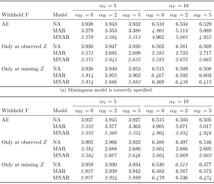
Table 2.1 Simulation study results of the three model variants analyzed on 50 generated datasets at 9 factor combinations. Results forαY = 0are not included because all models achieved the approximately the same RMSE, as expected. . . 15 Table 2.2 Root mean squared error (RMSE) of predictions vs. test set PM2.5measurements
(about 20% withheld from total observations). The lowest RMSE between all three models is italicized in each setting. . . 16
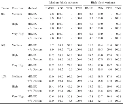
Table 3.1 Local test and estimation performance for MIMIX and MIMIX w/o Factors under a variety of simulation conditions as measured by root mean squared error (RMSE), coverage of 95% credible intervals (C95), true positive rate (TPR), and true negative rate (TNR). All values are multiplied by 100. . . 32
Table 4.1 Numerical summary of predictions overall and across several covariates by prediction error (km) and percent of prediction region coverage. . . 50
Table 5.1 Geolocation predictions within the continental United States using ambient dust-associated fungal microbiome data. . . 66 Table 5.2 Geolocation predictions within the Triangle region of North Carolina using
LIST OF FIGURES
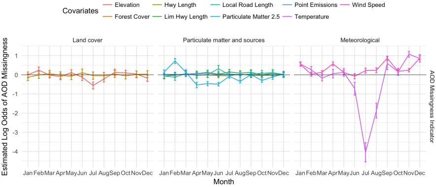
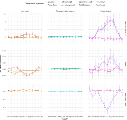
Figure 2.1 Per-month estimates of log odds of AOD missingness and 95% confidence intervals from the logistic regression of AOD missingness onto PM2.5and land cover, meteorological, and PM2.5 source covariates. Positive values suggest that as the value of the variable rises, so too does the probability that AOD is missing, while negative values suggest the reverse: as the variable rises, the probability that AOD is missing falls. . . 9 Figure 2.2 Fully observed values as generated in the simulation study at a single time
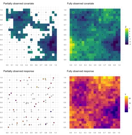
point with a moderate relationship betweenY and Z (αY = 5) and a mod-erate amount of informative missingness (αW = 2). The model is fit to the partially observed data, which aims to predict the response at locations where it is missing, while also accounting for missingness in the covariate. At a sin-gle time point, the response is only observed at a subset of the available monitoring stations (circles) in the region. Moreover, the spatial processes are modeled at a sparse collection ofL= 49knots (crosses) spread over the region. . . 13 Figure 2.3 Coefficient estimates for fully observed covariates at each month over 2003,
2004, and 2005. . . 18 Figure 2.4 Coefficient estimates for AOD and informative missingness at each month
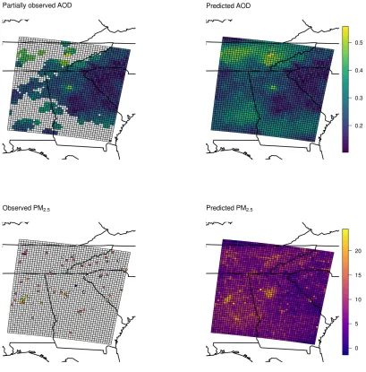
over 2003, 2004, and 2005. . . 19 Figure 2.5 PM2.5 and AOD observations on July 5, 2004 and predictions made by
MNAR model. . . 20
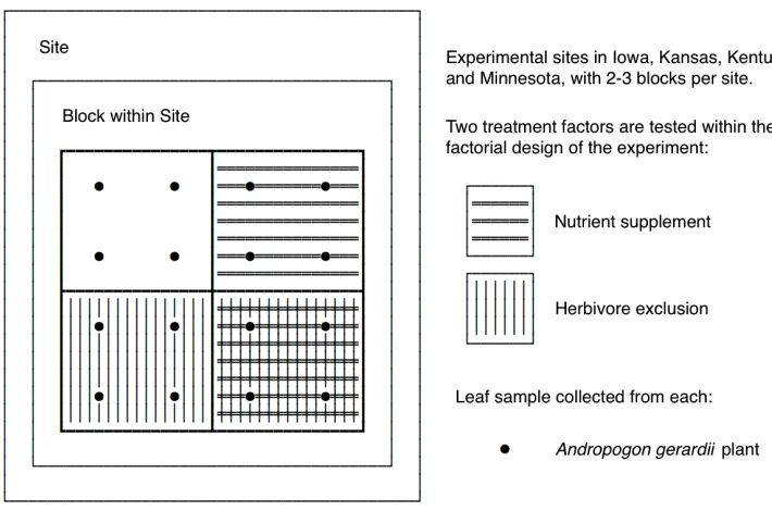
Figure 3.1 A schematic representation of the Nutrient Network experimental design. This experiment replicates a 2x2 RCB design across several sites. Four plants are sampled from each plot and a microbial sample is collected from each plant late in the growing season (August). . . 25 Figure 3.2 Results of a global test for treatment effect by MIMIX, MIMIX w/o Factors,
and PERMANOVA, under a variety of simulation conditions. When β =0
(0% Dense) the line gives the test’s type I error, where a dashed line at 0.05 is provided for reference. Forβ̸=0 (>0% Dense), the line values depict the statistical power of each test. . . 31 Figure 3.3 Posterior predictive checks on sparsity for MIMIX applied to the NutNet
Figure 3.4 Posterior 95% credible intervals for the effect of nutrient supplement on each OTU. Across all OTUs (a), most are not significantly affected by the treat-ment (gray lines), but MIMIX identifies 84 of 2,662 OTUs (3.2%) that show a significant response (black lines). Among these affected OTUs (b), the tax-onomy of each fungal OTU is given up to species, if known, or at a higher taxonomic rank, such as genus or order, with trailing numbers identifying distinct strains. The OTUs are ordered along the y-axis according to com-plete linkage hierarchical clustering of the estimated factor correlation matrix from MIMIX. . . 35 Figure 3.5 The proportion of variance for each OTU that is explained by the
contribu-tion of site and block vs. unexplained residual variacontribu-tion. Black dots corre-spond to OTUs identified by MIMIX as being significantly affected by nutri-ent supplemnutri-ent in Figure 3.4b, though only a subset of names are displayed to avoid overlapping labels. . . 36 Figure 3.6 Estimated factor correlation matrix among OTUs, with OTUs ordered by
hierarchical clustering. Clusters of strongly correlated OTUs, represented by purple triangles along the diagonal, indicate small collections of taxa that respond similarly to the fixed and random effects of the designed experiment. The OTUs highlighted along the diagonal are those identified by MIMIX as being significantly affected by nutrient supplement in Figure 3.4b, though only a subset of names are displayed to avoid overlapping labels. . . 37
Figure 4.1 A map of estimated occurrence probabilities of Eutypa lata, just one of our nearly 40,000 fungal taxa, communicates quite a bit about its spatial spread and prevalence. Each◦marks the location of a dust sample identifying signif-icant traces of Eutypa lata while an ×indicates sample locations where the species was absent. Kernel smoothing produces estimated occurrence proba-bilities ofEutypa lata, where areas with darker purple shading are more likely to produce samples containing traces ofEutypa lata. In our 928 samples, Eu-typa lata was found exclusively in the west near the grapevines on which it depends. This species has a 40-50% chance of appearing in a sample taken in the regions in which is it found. . . 47 Figure 4.2 The biogeography of Teratosphaeria microspora is much different than that
ofEutypa lata(Figure 4.1). The darker and more prevalent shading suggests Teratosphaeria microsporais a fairly common and widespread fungal taxon. However, it occurs with highest frequency among samples collected from the West Coast and throughout Midwestern regions bordering the Great Lakes. . 48 Figure 4.3 A sample taken in central Michigan is predicted to have originated from
northern Indiana, a prediction error of 229.3 km. This distance marks the median prediction error of our method’s 928 total predictions. . . 49 Figure 4.4 Histogram of prediction error for n = 928 predictions over five-fold cross
validation. . . 49 Figure 4.5 All 928 predictions produced by the model over five-fold cross-validation.
Figure 4.6 Summary of the spatial source prediction method. Given a database of se-quenced dust samples from known origins s1, . . . ,sn, kernel smoothing pro-duces taxon-specific “hot spot” maps like Figures 4.1 & 4.2. Using Bayes’ rule, our method combines these estimated occurrence probabilities with the sequenced taxa data observed in a new dust sample of unknown origin s0 to identify the sample’s most likely origin sˆ (red point). The enveloping prediction regions suggest broader areas where the sample is likely to have originated beyond a single “pin-in-a-map” point estimate. . . 53
Figure 5.1 Pointwise and regional predictions for a single sample made by Coarse DS at increasing numbers of classifier-partition pairs. . . 62 Figure 5.2 Voronoi partitions generated over the continental United States. Sample
points are labeled according to the cell they lie within and a supervised classifier is trained on these labeled data. Empty cells are ignored by the classifier. . . 63 Figure 5.3 State classification between Coarse DS and State DNN. Each plot depicts the
frequency of samples predicted to originate from a particular state (x-axis) against their true state of origin (y-axis). Because Coarse DS is designed to detect regional patterns, it appears to more often make predictions closer to the true state of origin (as evidenced by tighter clustering along the diagonal) compared with the State DNNs. . . 67 Figure 5.4 Prediction errors made by Coarse Spatial RF over ten-fold cross-validation.
Each arrow points in the direction to which a prediction is likely to be made, and the arrow’s color indicates how far that prediction is likely to be from the true origin, on average. . . 68 Figure 5.5 Prediction errors made by Coarse DS over ten-fold cross-validation. Each
arrow points in the direction to which a prediction is likely to be made, and the arrow’s color indicates how far that prediction is likely to be from the true origin, on average. . . 69 Figure 5.6 Prediction errors made by Coarse DS and County DNN over ten-fold
cross-validation. Each arrow points in the direction to which a prediction is likely to be made, and the arrow’s color indicates how far that prediction is likely to be from the true origin, on average. . . 71 Figure 5.7 Country classification between Mixed DS and Country DNN. Each plot
Chapter 1
Introduction
A microbiome is a community of microorganisms and their genomes that belong to a partic-ular ecological niche such as the human gut, soil, plants, or ambient dust. Samples collected from these habitats invariably contain thousands of archaea, bacteria, and fungi which may be identified through their DNA with next-generation sequencing technologies (Metzker, 2010). Understanding how these microbial communities interact with their environment holds signifi-cant implications for the fields of human health (Wu and Lewis, 2013), climate change (Bond-Lamberty et al., 2016), forensics (Giampaoli et al., 2014), and more. However, the tools available for characterizing microbiomes are, at present, largely limited to descriptive studies and must evolve to meet the advanced needs of the microbiome research community. To this end, the interdisciplinary Unified Microbiome Initiative (Alivisatos et al., 2015) aims to achieve “predic-tive understanding that allows evidence-based, model-informed microbiome management and design” by encouraging collaborative work on several promising areas of emphasis.
One such area of emphasis is the development of new statistical models for microbiome data analysis. Microbiome data are difficult to model because they are high-dimensional, sparse, over-dispersed, and possess complex dependence structure. Moreover, as a consequence of the next-generation sequencing technology, the data are compositional, meaning they convey relative rather than absolute information; a microbe’s abundance in a sample (the number of times its DNA was read by the sequencer) depends on the sequencing depth (the total number of reads). Most standard multivariate statistical methods are designed for the analysis of absolute information and will yield spurious correlations among variables when applied indiscriminately to compositional data (Pearson, 1896).
the geographic coordinates where each sample was collected which allows for the characteriza-tion of “biogeographies,” or microbial occurrence patterns as they relate to geographic regions (e.g., Barberán et al., 2015).
In this dissertation, we present a collection of models for the analysis of high-dimensional, spatially-distributed microbiome data in the context of two growing research areas within the microbiome domain. First, we contribute to the developing field of designed experiments for microbiome data where the primary goal is to detect treatment effects on microbial taxa while accounting for heterogeneous sources of variability. Second, we investigate the potential for microbiome data to guide forensic inquiry, finding that the microbial profile of a sample of ambient dust can be used to geolocate the spatial source of that dust with high precision.
1.1
Microbiome Data from Designed Experiments
Contemporary analysis of microbiome data often works on metrics that summarize collective properties of the entire microbiome, such as measures of taxonomic diversity. Among-sample diversity, referred to asβ-diversity, describes differences in taxonomic composition among sam-ples, and may be quantified by measures like Bray-Curtis dissimilarity (Bray and Curtis, 1957) or, if full taxonomic assignments are available, UniFrac distance (Lozupone and Knight, 2005). Permutational multivariate analysis of variance (PERMANOVA) with pairwise differences be-tween samples (McArdle and Anderson, 2001) is a popular tool to test whether environmen-tal covariates are associated with significant differences in these summary metrics. However, PERMANOVA does not yield inferences about the effects of environmental stimuli on specific microbial taxa.
Another option for the analysis of microbiome data is to model the proportions or counts of individual taxa as response variables in univariate mixed models. While potentially more effec-tive than PERMANOVA at detecting environmental effects, these methods fail to account for complex correlation patterns among microbial communities. Unlike univariate models, multi-variate models can pool information across taxa to increase power for detecting and estimating treatment effects. For example, the Dirichlet-multinomial (DM) model provides a rich frame-work for modeling the entire vector of raw abundance data in each microbiome sample and has proven useful in the areas of hypothesis testing and power calculations (La Rosa et al., 2012), sparse variable selection (Chen and Li, 2013), and inference of microbial community structure (Shafiei et al., 2015).
of unique taxa produced by next-generation sequencing technologies. To accommodate the high-dimensionality of microbiome data, we develop a hierarchical Bayesian model which relies on unobservable variables, or latent factors, to capture dependence patterns among thousands of microbial taxa.
In Chapter 2, we explore the use of a hierarchical Bayesian latent factor model to induce dependence between the value of a partially-observed spatial covariate and its missingness sta-tus. This initial analysis is motivated by atmospheric data on aerosol optical depth (AOD) and harmful particulate matter (PM2.5), and our model reveals statistically-significant informative missingness and relationships between PM2.5 and AOD in many seasons after accounting for meteorological and land-use variables. These results suggest that a latent factor model could prove useful in a more advanced setting that involves high-dimensional microbiome data.
To this end, we present a new Bayesian mixed-effects model for microbiome data analysis in Chapter 3 which we call MIMIX (MIcrobiome MIXed model). MIMIX achieves four scientific objectives: (1) global tests of whether experimental treatments affect microbiome composition; (2) local tests for treatment effects on individual taxa and estimation of such effects if present; (3) quantification of how different sources of variability contribute to the microbiome hetero-geneity; and (4) characterization of latent structure in the microbiome, which may suggest ecological subcommunities. MIMIX is a LNM mixed model that uses Bayesian factor analy-sis (Rowe, 2002) to capture complex dependence patterns among microbial taxa. Specifically, MIMIX models high-dimensional relationships among the transformed abundance probabilities of individual taxa through a set of low-dimensional unobservable variables, or latent factors. MIMIX naturally identifies clusters of microbes that respond similarly to experimental condi-tions by developing continuous shrinkage Dirichlet-Laplace priors (Bhattacharya et al., 2015) for these latent factors. We then apply Bayesian variable selection priors for the fixed effects on subpopulation abundance, reflecting the prior belief that treatments will not affect all ecological communities.
1.2
Forensic Geolocation using Microbiome Data
Forensic geolocation is the act of identifying the geographic source of an item based on its ob-servable properties. For example, forensic analysis of soil on a rug at a crime scene may provide clues to the geographic whereabouts of individuals involved. Another promising source of infor-mation for use in geolocation is ambient dust collected on buildings, objects, and individuals.
of all our movements and of all our encounters” (Locard, 1930). Realization of Locard’s vision has been slow, however. A primary reason is that dust analysis has historically relied on the identification of pollen grains (a laborious task) and knowledge of local plant geographies (often requiring specialized expert input) (Bryant and Jones, 2006). Recent work has expanded the capabilities of pollen for forensic analysis (Jones, 2012; Goodman et al., 2015), but the technique remains underutilized in practice.
In addition to pollen, dust typically harbors a myriad of other taxa, including large numbers of microbial taxa (Brodie et al., 2007) and there is some evidence that the analysis of these taxa can also be used to identify the geographic origin of dust or soil samples (Araujo et al., 2009; Giampaoli et al., 2014). Fungi represent a particularly promising taxon for geolocation and forensic analyses in general (Hawksworth and Wiltshire, 2011) for a variety of reasons. First, the global diversity of fungi is enormous with nearly 100,000 described fungal species and far more that remain undescribed (Blackwell, 2011) with individual samples of soil or dust harboring large numbers of fungal taxa (Bowers et al., 2013; McGuire et al., 2013). Second, many fungal taxa are restricted in their geographic distribution and are only found in particular locations or ecosystem types (Talbot et al., 2014). Third, since many fungal taxa produce spores that are tolerant of dessication and other environmental stresses they can persist in samples for prolonged periods of time. Despite the advantages of fungal analyses for geolocation, their utility remains more potential than realized and there are very few cases of fungi being used for forensic investigations (Hawksworth and Wiltshire, 2011). To facilitate the incorporation of fungal analyses into forensic work, we introduce statistical models that are capable of predicting the origin of a sample with high accuracy based solely on the sample’s unique collection of fungal taxa.
In Chapter 4, we develop a preliminary forensic geolocation model for fungal presence/absence data using Bayesian discriminant analysis (BDA) (Hastie et al., 2009). BDA is a two-stage clas-sification method built on Bayes’ Theorem that classifies a new observation as arising from one of many possible populations based on its measured characteristics. The analysis proceeded in two stages: using available samples, we first estimated the spatial distribution of each taxon’s oc-currence probability using Gaussian kernel smoothing, and then inverted these probabilities to predict the spatial origin of a new sample. When applied to the dust microbiomes of over 1,000 homes across the continental United States, the geolocation model makes point predictions that fall within 230 kilometers, on average, of their true origin.
Chapter 2
Spatial Regression with an
Informatively-Missing Covariate
2.1
Introduction
Fine particulate matter of<2.5µm in aerodynamic diameter (henceforth PM2.5) is a harmful air pollutant due to its ability to easily infiltrate human lungs and blood streams (EPA, 2009). Measurements of the concentration of PM2.5 in the atmosphere are sparse in both space and time; monitoring stations are predominantly located in large metropolitan areas where PM2.5 is likely higher and most impactful of human health and, due to cost considerations, stations tend only to take measurements once every few days. Statistical methods allow for predictions of PM2.5 at locations and times where it is unobserved. Such predictions have historically relied on land-use regression models which regress observed PM2.5 on corresponding land-use covariates such as elevation, forest cover, and distance to major road or highway (Ryan and LeMasters, 2007; Jerrett et al., 2005). As these covariates tend not to be temporally variable, land-use regression models successfully capture long-term PM2.5trends, but fail to account for short-term variations in daily PM2.5. Inclusion of temporally varying meteorological terms like temperature and wind speed can aid temporal predictions (Lindström et al., 2014), so too can aerosol optical depth (AOD) (Liu et al., 2005; Paciorek et al., 2008; Kloog et al., 2011; Lee et al., 2011; Chang et al., 2014). AOD derived by remote sensing can be particularly useful due to its large spatial coverage, though the extent of its utility in aiding PM2.5 prediction can vary across spatial scales, geographical regions, and satellite products.
AOD is a relatively new and useful covariate due to its fine spatio-temporal resolution; it has global imaging coverage and measurements are taken nearly two times a day. However, a down-side to AOD is that it may largely be missing at locations with high surface reflectivity (e.g. snow cover) and on days of significant cloud cover because the spectral bands used by MODIS to sense atmospheric aerosols cannot penetrate the clouds (Gupta and Christopher, 2008; Hoff and Christopher, 2009; Duncan et al., 2014).
Standard geostatistical analyses implicitly assume that sample locations and the data mod-eled at these locations arise from independent stochastic processes. There is an emerging lit-erature (Reich and Fuentes, 2012) on developing spatial methods to account for dependence between these processes. One form of dependence is preferential sampling (Diggle et al., 2010; Pati et al., 2011) where particular sample locations are observed over others because the true process is thought to be higher at these locations. For example, air pollutant monitoring sta-tions are densely located around large urban populasta-tions to ensure compliance with regulatory standards and protect public health, or mining stations are more likely located in areas of high-grade ore. Naïve modeling of air quality or ore high-grade in these respective scenarios yields biased results as data at the sampled locations are not representative of the region at-large.
Another form of dependence is informative missingness. In this case, the locations of the sample points are fixed, but some values are missing and this missingness is related to the underlying process of interest. When data are missing-at-random it is standard practice in spatial statistics to use Kriging techniques to impute the missing values. However, such an approach is not appropriate when the missingness is informative of the value unobserved at this location. For example, Reich and Bandyopadhyay (2010) show that the periodontal health of a patient is informed by both the number and locations of missing teeth by developing spatial methods for an informatively missing response.
In our application, AOD is a spatially missing covariate whose missingness status may be informative of its values and its relationship with its response, PM2.5(Yu et al., 2015). There has been some work on spatial models for missing covariates. Li et al. (2009) develop spatial linear mixed models for a covariate observed with measurement error. Huque et al. (2016) propose a semiparametric regression model which corrects for spatial covariates measured with error. With respect to AOD, Kloog et al. (2012) incorporate inverse probability weighting in their spatial model to address nonrandom missingness in AOD.
properly accounting for an informatively missingness can improve both spatial predictions and parameter estimation. Section 2.6 applies the models to the EPA monitoring and NASA satel-lite data in the Southeastern United States. Finally, we close with a discussion in Section 2.7. Full conditional distributions used in MCMC are detailed in Appendix A.
2.2
Data description and exploratory analysis
The study domain covers a portion of the Southeastern U.S. centered on Atlanta, GA and its surrounding metropolitan areas. Within the study domain, a network of 85 monitoring stations are maintained as part of the US Environmental Protection Agency (EPA) Air Quality System (AQS) which measure particulate matter concentration in the atmosphere. Twelve of the 85 stations (mostly those lying in closest proximity to urban areas) collect PM2.5 data every day, with the remaining stations taking measurements usually once every three days.
Daily satellite-derived AOD is available at up to 2,400 locations covering the spatial domain on a grid with a resolution of 12×12 km2 cells. AOD measurements are missing for 43% of observations. Additional covariate information are available at these locations. This includes land cover covariates: elevation (meters) and forest cover (proportion of grid cell covered by forested land); PM2.5 source covariates: highway length (total kilometer length of highways within grid cell), local road length (total kilometer length of local roads within grid cell), and point emissions sources; and meteorological covariates: wind speed (meters per second) and mean temperature (degrees celsius).
We conduct an exploratory analysis to investigate associations with AOD missingness by fitting a logistic regression model, temporarily ignoring spatial and temporal dependence. After assigning to each monitor the AOD value for the grid cell which contains the monitor, the logistic regression is performed with the binary response that AOD is missing or not at the monitor station regressed on an intercept, longitude and latitude (up to second order including interaction), PM2.5 concentration measurements, and the aforementioned covariates.
Figure 2.1: Per-month estimates of log odds of AOD missingness and 95% confidence intervals from the logistic regression of AOD missingness onto PM2.5 and land cover, meteorological, and PM2.5 source covariates. Positive values suggest that as the value of the variable rises, so too does the probability that AOD is missing, while negative values suggest the reverse: as the variable rises, the probability that AOD is missing falls.
wind speeds are indicative of weather patterns that may suggest cloud cover. Finally, in the presence of these other covariates, PM2.5 is associated with AOD missingness, with a positive association in the months January to March, and a negative association April to June, August, and October. Thus, these complex relationships motivate a careful analysis of the missingness pattern in AOD as part of our spatial regression model for PM2.5.
2.3
Statistical model
LetY(s)be the observed response at spatial locations. For notational convenience we describe the model for a single realization of the process; this is generalized in Appendix A to accommo-date multiple time points. We define two sets of covariates. Thep-vectorX(s)is assumed to be observed at all spatial locations, whereas Z(s), a scalar, is observed only partially. Define the missing data indicator asδ(s) = 1ifZ(s) is missing andδ(s) = 0otherwise. In our analysis, Y is PM2.5, X is a p-vector of land-use, meteorological, and human-derived covariates including an intercept and first- and second-order spatial terms, and Z is AOD.
We define the model for the response conditional on the covariate Z(s) as
whereαY is a scalar effect ofZ,θY is the spatial random effect, andϵY(s)iid∼ N(0, τY2)is random error. The spatial random effect is assumed to be a Gaussian process with mean E[θY(s)] =
X(s)TβY, variance V[θY(s)] = σ2Y, and correlation Cor[θY(s), θY(s′)] = ψ(d;ϕY), where d= ||s−s′|| and ψ is the spatial correlation function with parameters ϕY; collectively, we denote this model as θY ∼GP(βY, σY,ϕY).
Imputing the missing covariate values requires a model for Z. Accounting for informative missingness also requires a model for the missing data indicator δ(s). To facilitate a joint model, define δ(s) =I[W(s) >0], where W(s) is a latent continuous process that determines the locations of missing data. We use the joint model
Z(s) =θZ(s) +ϵZ(s) and W(s) =θW(s) +αWθZ(s) +ϵW(s), (2.2)
where θZ ∼ GP(βZ, σZ,ϕZ), θW ∼ GP(βW, σW,ϕW), ϵZ(s) iid
∼ N(0, τZ2), and ϵW(s) iid ∼ N(0, τW2 ). For identification purposes we fix V ar[W(s)] = σW2 +τW2 = 1, since only the sign and not the scale of W is identifiable. The presence of αW in (2.2) allows us to account for informative missingness by linking the values ofZ over our region of interest with their missing data status. If αW = 0 then the missing data indicator is independent of Y and Z, and can thus be ignored; ifαW >0 (αW <0) then observations with large values of θZ are more (less) likely to be missing, thus inducing dependence between the missing data indicator and the true value of the covariate.
2.4
Computational details
In our application, the monitoring data Y is available only at a small number of spatial loca-tions S˜={˜s1,˜s2, . . . ,˜sm}. LetY = [Y(˜s1), . . . , Y(˜sm)]′ and θY = [θY(˜s1), . . . , θY(˜sn)]′. The partially observed covariate Z and missing data process W are defined over a fine grid of n spatial locations (centroids of the grid cells)S ={s1,s2, . . . ,sn}. LetZ= [Z(s1), . . . , Z(sn)]′, W = [W(s1), . . . , W(sn)]
′
,θZ = [θZ(s1), ..., θZ(sn)]
′
, and θW = [θW(s1), ..., θW(sn)]
′
.
The joint likelihoods of θZ and θW involve cumbersome n×n matrix operations which present computational challenges. Low-rank models are a means of alleviating this computa-tional burden (Cressie and Johannesson, 2008; Fuentes, 2002). We employ the Gaussian predic-tive process (GPP) approach developed in Banerjee et al. (2008). For the spatial processes Z, we can reduce the dimension of the problem by constructing a smaller set ofLknotsv1, . . . ,vL. The spatial model is then defined over the knots asθ∗Z(v)∼GP(0, σZ,ψZ), and related to the original process as
where θ∗Z = [θ∗Z(v1), . . . , θ∗Z(vL)]T ∼ N(0,RZ), HZ = CZRZ−1, and CZ is the n×L matrix with (i, l) element ψ(||si−vl||,ϕZ). Placing L=n knots at then observation locations gives the initial full-rank model for the parent process Z, and taking L << n results in a low-rank and computationally-efficient approximation. However, we sacrifice some degree of predictive performance as the predictive processes are smoother than their parent processes (Finley et al., 2009). A similar approach is taken for the latent processW.
Parameter estimation and prediction of variables where and when they are unobserved rely on Markov chain Monte Carlo (MCMC) posterior sampling over 30,000 iterations with the first 10,000 removed for burn-in. The steps of the algorithm are given in Appendix A, where the variables are further indexed by t = 1, . . . , T to accommodate multiple time points. Many of the parameters in this hierarchical Bayesian model are conditionally conjugate with the proper choice of prior distribution. The variance parametersτY2,τZ2, σY2, and σ2Z, follow independent, uninformative inverse-gamma(0.1,0.1) priors, and σ2W is updated with a Metropolis-within-Gibbs step. The regression coefficientsβY,βZ, and βW have independentN(0,1000Ip)priors, and αY and αW have independent N(0,1000) priors. Furthermore, the spatial rangesϕY, ϕZ, and ϕW have non-conjugate posteriors and are given independent discrete uniform priors to ease computation. The support of each spatial range prior depends on the application: in the simulation study, which is performed over the unit square, the supports of ϕY, ϕZ, and ϕW begin at 0.2 and end at 5 in twenty equidistant increments. In the data analysis, the supports ofϕY andϕZ begin at 100 and end at 3000 in increments of 100, and the support ofϕW, which must be reduced due to the fixed variance ofW, begins at 10 and ends at 300 in increments of 10.
Computational analyses were performed in Julia (julialang.org) (Bezanson et al., 2017) and graphics were produced in R (R Core Team, 2013). Reproducible code is available at http://github.com/nsgrantham/spatial-covariate-informative-missingness.
2.5
Simulation study
We conduct a Monte Carlo simulation study to investigate the performance of our proposed method under different degrees of informative missingness, and to explore effects of model misspecification. The covariate process Zt and response process Yt are generated over a 21× 21 grid of cells (n = 441 total) with equidistant grid cell centers located at (−1.0,−1.0), (−0.9,−1.0), . . ., (0,0), . . ., (1.0,1.0) over independent time points t = 1, . . . ,10 . No other covariates are considered, so p= 1 and Xt(s) = 1 for alls andt.
captured by αY. αW is varied over 0, 2, and 5, and αY is varied over 0, 5, and 10. Other parameter values are fixed at βY = 10, σY2 = 16,τY2 = 4, ϕY = 0.5,βZ = 0, σZ2 = 2,τZ2 = 0.1, ϕZ= 0.5,βW = 0,σ2W = 0.9,τW2 = 1−σW2 = 0.1, andϕW = 3over the course of the simulation. In the first set of simulation studies, data are generated from the model described in Section 2.3 in the following way:
1. Spatial random effects are generated θZt ∼GP(0, σZ, ϕZ) and θWt ∼GP(0, σW, ϕW).
2. Conditional onθZt, eachZt(s)is independent overS and drawn fromN
[
µZt(s), τ
2 Z ]
with µZt(s) =Xt(s)βZ+θZt(s).
3. Conditional on both θWt and θZt, the latent factor Wt(s) is drawn independently from
N[µWt(s), τ
2 W
]
withµWt(s) =Xt(s)βW +µZ(s)αW +θWt(s).
4. Conditional onZtand spatial processθYt ∼GP(0, σY, ϕY), the responseYt(s)is
indepen-dent over S and drawn fromN[µYt(s), τ
2 Y ]
withµYt(s) =Xt(s)βY +Zt(s)αY +θYt(s).
5. These true values are not observed in their entirety, however. When active, the missing data status defined by δt(s) =I(Wt(s)>0)restricts direct observation ofZt(s).
6. Finally, to mimic the spatial sparsity in AQS monitoring stations in our motivating dataset, m = 50 monitors are placed at random over the domain, not necessarily at grid cell centroids, and at each time point tsome 50% of monitor values are observed to comprise responseYt.
Figure 2.2 depicts one time point of a dataset constructed in this way with αW = 2 and αY = 5. Low informative missingness means that the high values of the covariateZare not likely to be observed. Moreover, the response Y is weakly influenced by Z, but such a relationship may be difficult to infer from the sparse selection of Y observed over the grid.
It is important to study effects of misspecification of this aspect of the model because in practice verifying the form of this relationship will be difficult. Thus, in the second set of simulations, data are generated from a deviation from the model described in Section 2.3. The data-generating process follows the same steps as the first setting except that we alter the mean of the missing data mechanism in item 3 to be
µWt(s) =Xt(s)βW +g[θZt(s)]αW +θWt(s) (2.4)
for a non-linear functiong. Specifically, we consider the functiong[θZt(s)] =aI(θZt(s)>0) +b,
wherea,bare fixed so that Eg[θZt(s)] =Xt(s)βZ and V g[θZt(s)] =σ
2 Z.
1. Missing Not at Random (MNAR): The latent factor model as presented in 2.3 which allows for an informatively missing covariate.
2. Missing at Random (MAR): Missing values in the covariate are assumed to have arisen at-random and are filled in with Kriging. This is equivalent to fixingαW = 0in the latent factor model.
3. Not Available (NA): No missingness model is given and the covariate is not included in the analysis. This is equivalent to fixing αY = 0 in the latent factor model.
Methods are compared via root mean squared error (RMSE) for predicting the response
Y at the locations in the 21×21 grid for which Y is not observed, further broken down into locations where Zwas observed or missing. An unobserved Y(s) is predicted by the posterior predictive mean of Yats.
Table 2.1a summarizes the results from the first simulation setting. A moderate relationship betweenY and Z (αY = 5) limits the predictive performance of NA versus MAR and MNAR. The latter two models perform similarly when Z is missing-at-random (αW = 0) but diverge when Z is informatively missing (αW > 0). For αW > 0, MNAR achieves lower RMSE than MAR at locations where Z was observed, as well as where Z was missing, although in this latter case the two models collectively produce higher RMSE on average. Table 2.1b summarizes the results from the second simulation setting where the models are misspecified. The RMSE achieved by MNAR in this setting is similar to the first setting, though slightly higher, suggesting the model is relatively robust to misspecification.
2.6
Data analysis
Table 2.1: Simulation study results of the three model variants analyzed on 50 generated datasets at 9 factor combinations. Results for αY = 0 are not included because all models achieved the approximately the same RMSE, as expected.
αY = 5 αY = 10
WithheldY Model αW = 0 αW = 2 αW = 5 αW = 0 αW = 2 αW = 5
All NA 3.938 3.943 3.932 6.510 6.534 6.529
MAR 3.279 3.353 3.380 4.901 5.113 5.089
MNAR 3.278 3.294 3.313 4.902 5.001 4.955
Only at observed Z NA 3.930 3.947 3.920 6.502 6.581 6.569
MAR 2.571 2.695 2.699 2.585 2.723 2.717
MNAR 2.571 2.641 2.635 2.585 2.675 2.665
Only at missing Z NA 3.938 3.949 3.953 6.515 6.509 6.508
MAR 3.914 3.955 3.962 6.467 6.592 6.603
MNAR 3.914 3.886 3.883 6.469 6.438 6.415
(a) Missingness model is correctly specified.
αY = 5 αY = 10
WithheldY Model αW = 0 αW = 2 αW = 5 αW = 0 αW = 2 αW = 5
All NA 3.937 3.945 3.927 6.515 6.503 6.505
MAR 3.332 3.377 3.363 4.905 5.071 5.017
MNAR 3.332 3.360 3.324 4.904 5.034 4.946
Only at observed Z NA 3.905 3.966 3.932 6.488 6.497 6.546
MAR 2.584 2.688 2.686 2.604 2.686 2.695
MNAR 2.584 2.667 2.646 2.604 2.669 2.662
Only at missing Z NA 3.959 3.930 3.934 6.530 6.513 6.477
MAR 3.937 3.939 3.942 6.482 6.587 6.573
MNAR 3.937 3.924 3.899 6.479 6.536 6.474
(b) Missingness model is misspecified.
2.6.1 Cross-validation
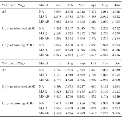
We validate model performance by withholding a subset of PM2.5monitor readings (20%) span-ning each monthly period over three years and comparing each model’s predictions against the actual PM2.5 values observed at these monitors. Specifically, we further examine the predictions by those made where AOD was or was not observed, as we anticipate MNAR may show better PM2.5 predictions at locations where AOD was missing.
Table 2.2: Root mean squared error (RMSE) of predictions vs. test set PM2.5 measurements (about 20% withheld from total observations). The lowest RMSE between all three models is italicized in each setting.
Withheld PM2.5 Model Jan Feb Mar Apr May Jun
All NA 3.695 3.606 3.642 3.477 4.081 4.056
MAR 3.678 3.588 3.624 3.488 4.046 4.123 MNAR 3.682 3.608 3.602 3.461 4.050 4.025
Only at observed AOD NA 4.297 3.107 3.345 3.780 4.299 4.552 MAR 4.281 3.073 3.312 3.792 4.223 4.558 MNAR 4.292 3.144 3.309 3.774 4.249 4.475
Only at missing AOD NA 2.847 3.890 4.091 2.888 3.823 3.373 MAR 2.826 3.879 4.095 2.897 3.839 3.536 MNAR 2.817 3.874 4.047 2.848 3.816 3.415
Withheld PM2.5 Model Jul Aug Sep Oct Nov Dec
All NA 4.189 4.863 4.843 4.350 3.067 3.839
MAR 4.179 4.919 4.862 4.221 3.048 3.792 MNAR 4.175 4.870 4.865 4.227 3.036 3.809
Only at observed AOD NA 3.794 4.653 5.227 4.680 3.163 4.164 MAR 3.828 4.793 5.175 4.530 3.140 4.124 MNAR 3.826 4.740 5.193 4.552 3.134 4.129
Only at missing AOD NA 4.611 5.110 4.126 3.765 2.902 3.286 MAR 4.558 5.069 4.290 3.674 2.889 3.224 MNAR 4.552 5.026 4.263 3.648 2.867 3.265
2.6.2 Inference and predictions
We further compare the coefficient estimates of the three models to draw inference on the relationship between the covariates and PM2.5and, where possible, AOD and AOD missingness. Of particular interest is the relationship between PM2.5 and AOD for the MAR and MNAR models which include AOD as a covariate, as well as the degree of informative missingness present estimated by MNAR.
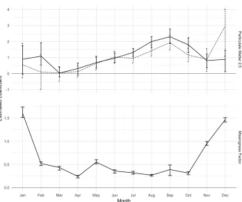
Figure 2.3 depicts the posterior mean and 95% posterior credible interval bounds for βY (first row), βZ (second), andβW (third) broken down by land-use, human-derived, and mete-orological covariates. Of the fully observed spatial covariates considered here, temperature is the strongest predictor of PM2.5 (Y), especially in the spring and summer months. Two other covariates show occasional significance in predicting PM2.5: elevation is slightly positively as-sociated May through September, and wind speed is slightly negatively asas-sociated for several months throughout the year. Human-derived covariates do not appear helpful in predicting PM2.5. Coefficient estimates largely agree between all three covariate missingness models.
AOD (Z) is also strongly predicted by temperature, though the wide credible intervals show this relationship is not quite so well-determined. MNAR and MAR both identify a marginally significant relationship between wind speed and AOD, with negative association in April and June, and a positive association in October. MNAR further identifies a strong negative asso-ciation in July. Land-use covariates appear to be good predictors of AOD, though MAR does not appear to estimate their utility quite so strongly as does MNAR. Elevation shows, at times, a weak positive association in the winter and spring months, and a relatively strong negative association in the summer and fall months. Forest cover is predominately negative in its rela-tionship with AOD, with its strongest estimates in February, March, and April. Human-derived covariates once again do not appear to be helpful predictors.
Finally, some spatial covariates are predictive of the AOD missingness factor (W) as esti-mated by MNAR. The coefficient estimates mimic those obtained by the exploratory logistic regression in Figure 2.1, suggesting the latent factor portion of the MNAR is indeed capturing the nature of missingness observed in the data. Temperature is the most notable predictor of missingness in all months but April and November. Wind speed and elevation show very small positive associations with missingness in a handful of months over the year, while forest cover along with the human-derived covariates show no association.
iden-tifying a significant relationship in February where MAR does not, and MNAR estimating a much weaker relationship in December than MAR. The reason for this latter disagreement may be explained by the large degree of informative missingness estimated by MNAR in Decem-ber, though it also produces high estimates in November and January which do not appear to cause a discrepancy in the estimation of αY between the models during these months. MNAR
Figure 2.4: Coefficient estimates for AOD and informative missingness at each month over 2003, 2004, and 2005.
estimates a consistent, positive relationship between AOD and its missingness status, suggest-ing that AOD is an informatively misssuggest-ing covariate and models which incorporate AOD as a predictor of PM2.5ought to account for this.
Figure 2.5: PM2.5 and AOD observations on July 5, 2004 and predictions made by MNAR model.
2.7
Discussion
informa-tively missing relationship between AOD and PM2.5 which appears to improve PM2.5 prediction at locations where AOD is missing, though this does not reliably translate to an improvement in PM2.5 prediction at all locations.
There are a couple explanations as to why improvements made by our model in the esti-mation of AOD where it is unobserved do not improve PM2.5 prediction. Most notably, after accounting for land-use and meteorological effects on PM2.5 , the effect of AOD on PM2.5 is simply not great enough to improve prediction where and when PM2.5 is unobserved. It may also be the case that a stronger link between AOD missingness and PM2.5levels is necessary for our latent factor model to improve upon the prediction performance of models which assume the covariate is missing-at-random or do not include the covariate at all.
Funding
Chapter 3
Bayesian Mixed-Effects Model for
Designed Experiments
3.1
Introduction
Contemporary analysis of microbiome data often works on metrics that summarize collective properties of the entire microbiome, such as measures of taxonomic diversity. For example, in ecology, within-sample diversity is most simply measured as the mean number of unique taxa observed in a sample, referred to asα-diversity. Among-sample diversity, referred to asβ -diversity, describes differences in taxonomic composition among samples, and may be quantified by measures like Bray-Curtis dissimilarity (Bray and Curtis, 1957) or, if full taxonomic assign-ments are available, UniFrac distance (Lozupone and Knight, 2005). Permutational multivariate analysis of variance (PERMANOVA) with pairwise differences between samples (McArdle and Anderson, 2001) is a popular tool to test whether environmental covariates are associated with significant differences in these summary metrics. However, PERMANOVA does not yield infer-ences about how the environment affects individual microbes. Additionally, implicit assump-tions made by such distance-based multivariate methods may be inappropriate for ecological count data altogether (Warton et al., 2012).
gamma-Poisson, are quite robust for this purpose and possess added flexibility for overdispersed data (Zhang et al., 2017).
An alternative to these univariate approaches is to model taxa within the microbiome jointly rather than individually. Unlike univariate models, multivariate models can pool information across taxa to increase power for detecting and estimating treatment effects. Towards this end, the Dirichlet-multinomial (DM) model — the multivariate extension of beta-binomial — provides a rich framework for modeling the entire vector of raw abundance data in each microbiome sample. For example, the DM has proven useful for microbiome analysis in the areas of hypothesis testing and power calculations (La Rosa et al., 2012), sparse variable selection (Chen and Li, 2013), and inference of microbial community structure (Shafiei et al., 2015). Despite their utility, Dirichlet variates have the undesirable property that they must negatively co-vary, making them ill-suited for modeling microbial taxa that often have positive associations, perhaps because they share similar habitat niches or because they interact symbiotically.
A more flexible dependence structure among microbial taxa is provided by Xia et al. (2013), who use a logistic normal multinomial (LNM) model that links the multinomial probability vector to a multivariate normal random variable, resulting in unconstrained occurrence prob-abilities on the linked scale. The covariance structure specified by Xia et al. (2013) captures both positive and negative associations among taxa, unlike the DM covariance. However, while suitable for small collections of taxa, their method for estimating this dependence structure is infeasible for high numbers of unique taxa produced by next-generation sequencing technologies. Further, they employ a penalized regression approach to test for environmental effects, which is not conducive to uncertainty quantification. Mixed-model versions of the DM and LNM needed to analyze experiments following split-block designs have yet to be developed for microbiome data, owing to the difficulty of introducing random effects into the model hierarchy.
priors for the fixed effects on subpopulation abundance, reflecting the prior belief that treat-ments will not affect all ecological communities. These objectives and features of MIMIX are motivated by a multi-location randomized complete block design (RCBD) experiment that seeks to identify the influence of nutrient supplement and herbivory on the foliar fungal microbiome of a common perennial prairie bunchgrass.
Section 3.2 introduces the data that motivate our development of MIMIX in Section 3.3. Section 3.4 demonstrates our method on simulated data in comparison with competing micro-biome data analysis methods. Finally, we apply MIMIX to RCBD experiment data in Section 3.5 and close with a discussion in Section 3.6. Details of posterior sampling schemes are left to Appendix B, and open-source code to reproduce the statistical analyses in this paper is available online athttps://www.github.com/nsgrantham/mimix.
3.2
Motivating Data
The Nutrient Network (NutNet,www.nutnet.org) is a global research cooperative hosted at the University of Minnesota that uses a standardized experimental protocol to study the impact of human activity at over 100 grassland sites spanning 6 continents (Borer et al., 2014). This article is motivated by data collected at 4 of these sites, all in the central US (Iowa, Kansas, Kentucky, and Minnesota). Each of these 4 sites features a 2 × 2 factorial experiment that crosses a nutrient-supplement treatment (i.e., fertilization) with an herbivore-exclusion treatment in a randomized complete block design (RCBD) (Figure 3.1). Here, we consider the effect of the two experimental treatments on the foliar fungal microbiome of Andropogon gerardii, a perennial bunchgrass found at each site, and native to prairie ecosystems of central North America.
NutNet scientists collected and prepared these data as follows. In August 2014, leaf samples were collected from fourA. gerardiiindividuals in each treatment plot. Samples were collected from plots in three replicated blocks, except in Iowa whereA. gerardii was present in only two blocks. Ten samples were later removed from the study due to errors during sequencing, leaving a total of 166 samples. Once collected, leaves were stored at 4 ◦C until surface sterilization. All leaves were surface sterilized within 24 hours after collection by exposing them to 1 minute each of 5% sodium hypochloride (bleach), 75% ethanol, and sterile distilled water. Leaves were then stored at -80 ◦C until DNA extraction.
The microbiome from each sample was characterized using a standard metagenomics ap-proach. Each surface-sterilized leaf was ground in liquid nitrogen, after which total genomic DNA was extracted using the Qiagen Plant Mini Extraction Kit (Qiagen). Genomic DNA was standardized to 20 ng/µL. The Roche FastStart High Fidelity Taq (Roche, Indianopolis, IN, USA), described in Nguyen et al. (2016), was used to generate fungal genomic libraries.
sequenced. Unique 7-bp sequences derived from NextGen Sequencing were used to barcode samples, as described in Smith and Peay (2014) and Nguyen et al. (2016). Triplicate PCR reactions were done with annealing temperatures of 51, 53 and 55◦C, and amplicons were pooled for each sample, purified using the QIAQuick Purification Kit, and quantified using a Qubit fluorometer and Quant-iT® dsDNA HS Assay kit (Thermo Fisher). Equimolar concentrations of purified libraries (25ng) were pooled and sequenced in Illumina MiSeq at the University of Minnesota Genomics Center (UMGC).
Operational taxonomic units (OTUs) were identified by clustering sequences with 97% similarity. All samples were simultaneously analyzed using a metagenomic pipeline adapted from Nguyen et al. (2016). Distal priming/adapter sites were removed with cutadapt v1.7.1 (Martin, 2011), and reads were trimmed using Trimmomatic v0.32 (Bolger et al., 2014). All short sequences or those with ambiguous bases were removed using the screen.seqs method of Mothur v.1.34.4 (Schloss et al., 2009). All remaining sequences were binned into oper-ational taxonomic units (OTUs) with 97% similarity using a pipeline adapted from Song (https://github.com/ZeweiSong/FAST).
Preliminary OTU assignments were performed using the UNITE fungal database v7.0 with BLAST v2.2.28+ (Camacho et al., 2009). Poor BLAST alignments (hit length <80% of the
alignment length, or percent identity <80%) were removed. OTUs assigned to Incertae sedis at the class level were reassigned based on taxonomic information at other levels; those that could not be reassigned were categorized as “unidentified.” We emphasize that these OTU assignments are preliminary and are subject to revision as reference libraries are updated, and as fungal phylogeny is more deeply understood. Accordingly, specific ecological findings presented in this article are also preliminary, and the definitive ecological analyses of these data will be provided in forthcoming work. Nevertheless, these data are suitable for fueling the methodological advances that we describe here. Overall, 2,662 fungal OTUs were identified across the 166 leaf samples. Samples harbored an average of 200 unique OTUs, and many OTUs were rare, as 85% of OTUs were identified in<10% of samples.
Given the preliminary OTU assignments, we wish to investigate each of the following using these data. First, we seek to characterize how the experimental treatments affect microbiome communities. We perform this analysis in stages: first at a global level where the response is the composition of the microbiome community as a whole, and then (if the global test identifies a significant treatment effect) at a local level that characterizes the effects on the relative abundance of individual OTUs. Second, we wish to characterize how the residual variation in the microbiome composition varies among blocks within sites and across sites, as quantifying these sources of variation may suggest insight into the ecological processes controlling these microbial communities. Finally, we wish to characterize the dependence structure among OTUs, and identify clusters of OTUs that may suggest underlying ecological subcommunities.
3.3
Methods
LetYik denote the count for samplei= 1, . . . , nand taxonk= 1, ..., K, and letmi= ∑K
k=1Yik be the total counts for samplei. The value of mi is an artifact of the sequencing depth of the high-throughput sequencing process and thus analyses are performed conditional on its value. For observationi, let xi be ap-vector of covariates and let zi∈ {1, . . . , q}record the source of the random effects from one of q blocking factors. This latter notation may be generalized to accommodate arbitrarily complex blocking designs, but for notational simplicity we assume a single blocking factor in this initial development.
A multinomial likelihood is natural for multivariate count data, so we takeYi= (Yi1, ..., YiK)′ ∼ Multinomial(mi,ϕi) where ϕi = (ϕi1, ..., ϕiK)′ is the vector of expected proportions with ϕi ∈ SK = {(ϕ1, . . . , ϕK)′ : ϕk ≥ 0, k = 1, . . . , K,
∑K
1986)
ϕik=ϕk(θi) =
exp(θik) K
∑
l=1
exp(θil)
for k= 1, . . . , K. (3.1)
There is a loss of dimension in transforming from RK to SK due to the latter’s unit-sum constraint, so to achieve identifiability we restrict eachθik to have prior mean zero.
In the spirit of Billheimer et al. (2001), we associate fixed and random effects with the microbiome composition through the mean of θi. The mixed effects decomposition is given by θi=µ+βxi+γzi+ϵi, whereµ= (µ1, . . . , µK)
′ is the overall population mean,β is aK×p
matrix of unknown fixed effect coefficients, γr is a K-vector of random effects from block r, and ϵi
iid
∼NK(0,Ω) is sample-specific random variation.
The number of taxa,K, is often very large in microbiome compositions. To address compli-cations due to high dimensionality and to account for relationships among taxa, we use Bayesian factor analysis (Rowe, 2002) to model the fixed and random effects within a lower dimensional representation. For a number of factors L, let Λ = (λ1, . . . ,λL) be the K ×L latent factor loading matrix, unknown and to be estimated. SupposeΛ is common to all fixed and random components of the model, a rather strong assumption, but one that allows each latent factorλl, l= 1, . . . , L, to capture sets of taxa correlated in their response to the model’s covariates and other sources of variability. Letβ=Λb,γr=Λgr,r = 1, . . . , q, andϵi =Λei+δi,i= 1, . . . , n. Thus, we may represent θi = µ+Λfi+δi where fi = bxi +gzi +ei is the low-dimensional
factor score vector for sample i.
A prior on Λ should ensure that the factor loading matrix captures common, cross-species covariance that lends itself to post-hoc inference of collective taxa responses. For instance, setting entire columns of Λ to zero is a means of selecting the number of active factors and setting individual elements within Λ to zero allows the factors to represent subsets of taxa (Carvalho et al., 2008). To achieve both forms of sparsity, we place continuous shrinkage priors on the high-dimensional factor loadingsλl, l = 1, . . . , Lcomprising Λ. In particular, we select a Dirichlet-Laplace prior (Bhattacharya et al., 2015) for its ability to detect sparse signals in high-dimensional linear regression, which we modify here for factor analysis. For factorsl= 1, . . . , L, let λl∼DLal represented by