ABSTRACT
WEATHERFORD, SHAWN A. Student Use of Physics to Make Sense of Incomplete but Functional VPython Programs in a Lab Setting. (Under the direction of Ruth Chabay.)
Computational activities in Matter & Interactions, an introductory calculus-based physics course, have the instructional goal of providing students with the experience of applying the same set of a small number of fundamental principles to model a wide range of physical systems. However there are significant instructional challenges for students to build computer programs under limited time constraints, especially for students who are unfamiliar with programming languages and concepts. Prior attempts at designing effective computational activities were successful at having students ultimately build working VPython programs under the tutelage of experienced teaching assistants in a studio lab setting. A pilot study revealed that students who completed these computational activities had significant difficultly repeating the exact same tasks and further, had difficulty predicting the animation that would be produced by the example program after interpreting the program code.
While working in groups over the course of a semester, study participants were recorded while they completed three activities using these incomplete programs. Analysis of the video data showed that study participants had little difficulty interpreting physics quantities, gen-erating a prediction, or determining how to modify the incomplete program. Participants did not base their prediction solely from the information from the incomplete program. When participants tried to predict the motion of the objects in the simulation, many turned to their knowledge of how the system would evolve if it represented an analogous real-world physical system. For example, participants attributed the real-world behavior of springs to helix ob-jects even though the program did not include calculations for the spring to exert a force when stretched. Participants rarely interpreted lines of code in the computational loop during the first computational activity, but this changed during latter computational activities with most participants using their physics knowledge to interpret the computational loop.
c
Copyright 2011 by Shawn A. Weatherford
Student Use of Physics to Make Sense of Incomplete but Functional VPython Programs in a Lab Setting
by
Shawn A. Weatherford
A dissertation submitted to the Graduate Faculty of North Carolina State University
in partial fulfillment of the requirements for the Degree of
Doctor of Philosophy
Physics
Raleigh, North Carolina 2011
APPROVED BY:
Robert Beichner David McConnell
John Risley Ruth Chabay
DEDICATION
This body of work is dedicated in loving memory and honor of
Christopher Price Weatherford
BIOGRAPHY
Shawn Weatherford was born in Norfolk, Virginia to Randy and Pam Weatherford on September 18, 1979. After moving to Corapeake, North Carolina, a small rural farm town at age 4, Shawn completed his entire grade school education in the Gates County Public School system. After graduating with a high school diploma, Shawn enrolled into a bachelor’s degree program at Elon College in Elon College, North Carolina to focus study in secondary science education and physics. As a North Carolina Teaching Fellow at Elon, Shawn was privy to internship experiences in Washington, D.C. and a semester in London, England. After adapting to the culture shock in public policy towards secondary education in England, Shawn returned to the States and joined the North Carolina Section of the Association of Physics Teachers. The following semester, he began a student teaching semester at Walter M. Williams High School in Burlington, North Carolina. Shawn was offered the physics teaching job at Williams upon graduating from Elon in 2001.
enjoyed revisiting old and forgotten skills as well as learning new physics that was previously beyond his reach. After joining the Physics Education Research and Development group, he turned his research focus on the component of physics instruction that refreshed his interest in physics: computation. Under the direction of Ruth Chabay and the support of the faculty in the PERD group, Shawn picked a research focus that, to this day, remains as exciting as it did at the beginning of his training.
ACKNOWLEDGEMENTS
Although there’s only one author on the title page, there’s a massive supporting cast behind the work to whom I owe a tremendous amount of gratitude that I will attempt to acknowledge. First, I should acknowledge the Physics Education Research and Development group for their willingness to have thoughtful conversations about my research and and endless amount of support. Ruth Chabay has been such an encouraging mentor and colleague and has provided endless support for this research as well as my desire to serve as a contributing member of AAPT. Bruce Sherwood, the person who introduced me to Matter & Interactions many years ago through a NCS-AAPT presentation and later my instructor for the course, was always excited about showcasing new features of Visual or a new demo to measure the effects of surface charge on a thin strip of aluminum foil. I appreciate Bob Beichner for his support to attend the Gordon Research Conference on computational physics in the physics curriculum which has had a substantial influence on my research and greatly increased my network of researcher contacts. I also owe Dr. Beichner thanks for exposing me to SCALE-UP and allowing me to serve as his TA. Thanks to John Risley and the team at WebAssign for the experience coding questions during two summers. I should note that there’s no conflict of interest: I ended my employment at WebAssign two years before I asked Dr. Risley to serve on my committee. And thanks to David McConnell for his willingness to provide time to serve on my committee and offer substantive comments on the research as well as bring his expertise in the affective domain. The faculty and staff in the NCSU physics department has been very supportive of this research and I thank specifically David Brown, Karen Daniels, David Haase, Jenny Allen for their assistance and guidance during my graduate program.
Jon Gaffney both served as great mentors through their willingness to involve my participation in their own research projects. Mary Bridget Kustusch has always been there to listen and talk about life’s unexpected traumatic events. Jeff Polak, Brandon Lunk, and Meghan West have all been willing to help validate the coding scheme and serve as independent raters for reliability measurements.
I offer a great amount of thanks to the officers and members of the North Carolina Section of the American Association of Physics Teachers. Over the past 13 years, I have enjoyed my membership to the organization and the many section meetings I’ve attended from across the state from Pembroke to Boone. Perhaps the most difficult part of moving away from North Carolina is moving out of driving distance from these meetings. The section has time after time supported my own scholarship and professional development through lunch conversations, presentations, and workshops. The opportunity to present my research and ideas over the years has provided public speaking practice that has had an ample effect on my performance. The section has provided leadership opportunities and provided a great amount of trust to allow a graduate student to plan and run a joint section meeting with the Southeast Section of the American Physical Society. Mario Belloni, Wolfgang Christian, Tony Crider, Jose D’Aruda, Joe Heafner, John Hubisz, Martin Kamela, Tatlock Lauten, Don Smith, Gordon Sheppard, Aaron Titus, Larry Ward have all offered wonderful conversation on the teaching and learning of physics.
Finally, I’d like to offer thanks to my support network outside of academics. Peter Dittmar, my partner and the best thing that’s come out of my graduate studies, has always had time to listen and offer optimism during difficult times when I had none. My parents who have been extremely supportive of my decision to interrupt my professional career to go back to school and who always offer a warm and inviting retreat from the city. Tanner, the puppy who is always excited to see papa come home even if he’s wearing a frown has always reminded me of the joys of life and the fleeting moments we have in it.
looked up to his older brother. His encouragement pushed me to strive farther and work on setting a better example. Chris was quite amused by calling me Dr. Weatherford before his passing and he’s still pushing me to this day to make every moment of this life count.
TABLE OF CONTENTS
List of Tables . . . xi
List of Figures . . . xii
Chapter 1 Introduction . . . 1
1.1 Terminology . . . 6
Chapter 2 Literature Review . . . 9
2.1 Introduction . . . 9
2.2 Computation in Introductory Physics . . . 10
2.2.1 Computational Thinking . . . 10
2.2.2 21st Century Curriculum Re-Design . . . 11
2.2.3 Computer-Based Modeling Environments . . . 12
2.2.4 Multiple Representations . . . 32
2.3 Program Comprehension . . . 39
2.3.1 Introduction . . . 39
2.3.2 Cognition and Comprehension . . . 39
2.4 Sensemaking in Physics Education Research . . . 44
2.4.1 Sensemaking in Physics Education Research . . . 46
2.5 Where does this leave us? . . . 51
Chapter 3 Pilot Study . . . 54
3.1 Participants . . . 54
3.2 Environment . . . 55
3.3 Procedure . . . 56
3.4 Results . . . 59
3.4.1 Task 1a - Study Program . . . 59
3.4.2 Task 1b - Predict Visual Output . . . 64
3.4.3 Task 1c - Run the Program . . . 68
3.4.4 Task 2 - Change the program to produce a circular orbit . . . 71
3.5 Discussion . . . 75
3.5.1 Link to Reading Comprehension . . . 76
Chapter 4 Methodology . . . 80
4.1 Motivating a new instructional tool . . . 80
4.1.1 A Minimally Working Program . . . 83
4.1.2 Instructional tasks using the MWP . . . 87
4.1.3 Empirical observations of a Spacecraft-Earth MWP test-run . . . 88
4.2 Design of the Experimental Study . . . 90
4.2.1 Qualitative Education Research Lab Environment . . . 90
4.2.3 Participants . . . 93
4.2.4 Integrating the MWP activities into the lab calendar . . . 94
4.2.5 Texture of the Data . . . 97
4.3 Methodology for Data Analysis . . . 98
4.3.1 Line-Number Coding . . . 101
4.3.2 Sensemaking Coding Scheme . . . 102
4.3.3 Action Coding . . . 103
4.3.4 Focus Coding . . . 106
4.3.5 Reliability and Validity Testing . . . 110
Chapter 5 Results . . . .112
5.0.1 Data Plots . . . 112
5.1 Spacecraft-Earth MWP . . . 115
5.1.1 Study/Prediction Task . . . 116
5.1.2 Running the program: Interpreting the visual output and evaluating pre-dictions . . . 143
5.1.3 Defining the modification goal . . . 146
5.2 Mass-Spring MWP . . . 154
5.2.1 Study/Prediction Task . . . 157
5.2.2 Running the program: Interpreting the visual output and evaluating pre-dictions . . . 184
5.2.3 Defining the modification goal . . . 189
5.3 Rutherford Scattering MWP . . . 193
5.3.1 Study/Prediction Task . . . 195
5.3.2 Running the program: Interpreting the visual output and evaluating pre-dictions . . . 224
5.3.3 Defining the modification goal . . . 228
5.4 Comparisons across all MWPs . . . 239
5.4.1 Interpreting and Predicting a MWP . . . 239
5.4.2 Evaluating the Prediction . . . 247
5.4.3 Modification Goals . . . 249
5.4.4 Logistics of completing the tasks . . . 250
Chapter 6 Conclusions. . . .254
6.1 Using Physics Knowledge . . . 255
6.2 Real-World Expectations . . . 256
6.3 Effect of research findings on the design of instructional activities . . . 257
6.3.1 Effect of findings on the development of VPython . . . 258
6.4 Future Work . . . 259
References . . . 261
Appendices . . . .270
Pilot Script . . . 271
Spacecraft-Earth MWP pilot in Spring 2009 . . . 275
Spacecraft-Earth MWP instructional document . . . 277
Spacecraft-Earth MWP code . . . 280
Mass-Spring MWP instructional document . . . 281
Mass-Spring MWP code . . . 285
Rutherford Scattering MWP instructional document . . . 286
Rutherford Scattering MWP code . . . 288
Experimental lab section seating charts . . . 289
LIST OF TABLES
Table 2.1 Table II from Hogan and Thomas(2001). . . 21
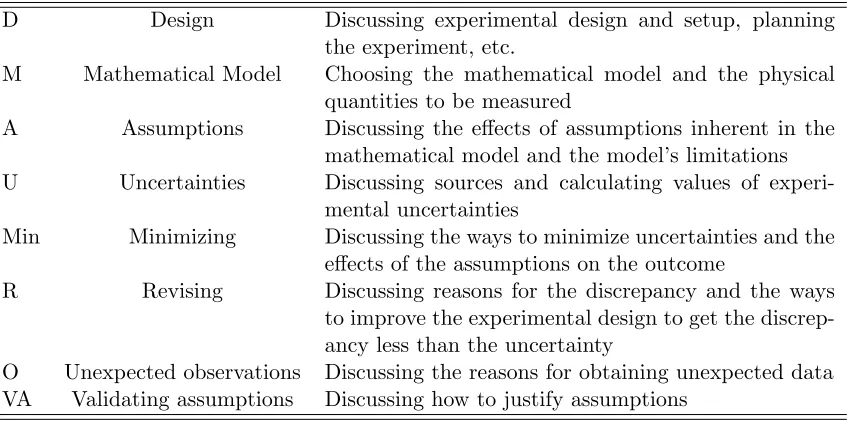
Table 2.2 Sense-making codes from Karelina&Etkina (2007). . . 51
Table 3.1 Pilot Study Tasks. . . 56
Table 3.2 Student Actions taken with each pilot study task . . . 77
Table 4.1 Comparison of the physical system to the features of the computational model which are included and omitted from the MWP. . . 84
Table 4.2 Demographics data of participant’s gender for the experimental lab sections. 94 Table 4.3 Lab activity schedule for experimental and traditional lab sections during the Fall 2009 semester. . . 95
Table 4.4 Reliability Measures for Coding Schemes . . . 111
Table 5.1 Group Membership by MWP Activity. Boldface denotes the Recorder . . 113
Table 5.2 Interpreting sections of code across all groups . . . 138
Table 5.3 Interpreting sections of code across all groups . . . 184
Table 5.4 Initial focus of groups beginning the modification task . . . 190
Table 5.5 Interpreting sections of code across all groups for the Rutherford Scatter-ing MWP . . . 223
Table 5.6 Number of groups interpreting the computational loop across all MWP activities . . . 243
Table 5.7 Interpretation strategies across all MWP activities . . . 244
Table 5.8 Source for information informing a whiteboard prediction across all MWP activities . . . 245
LIST OF FIGURES
Figure 1.1 Buffler’s model for computational activities in physics (Buffler et al, 2008,
p.432). . . 3
Figure 1.2 New model for computational activities in physics beginning with a com-prehension task. . . 4
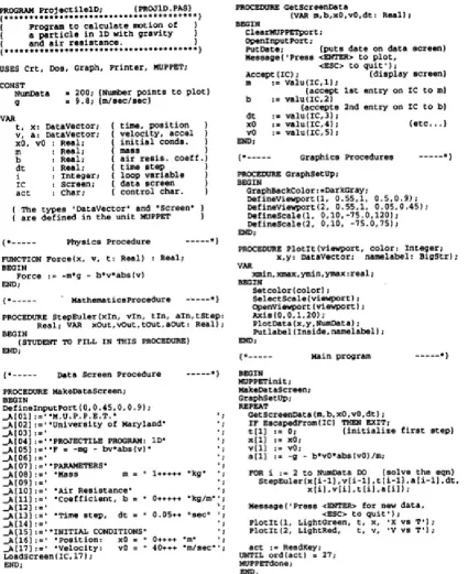
Figure 2.1 Source code for Pascal program modeling projectile motion(Redish & Wilson, 1993) . . . 14
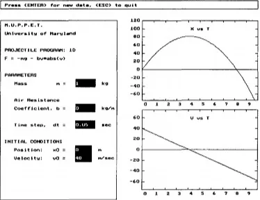
Figure 2.2 Input/Output screens from projectile motion program (Redish & Wilson, 1993) . . . 15
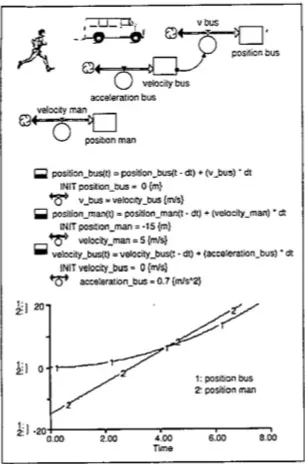
Figure 2.3 The STELLA model (top), the equations and procedures (middle), and output . . . 17
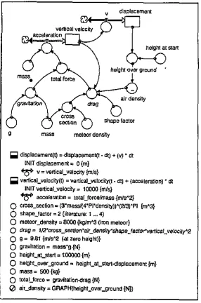
Figure 2.4 STELLA model for an asteroid moving through Earth’s atmosphere. (Schecker, 1993) . . . 20
Figure 2.5 A Boxer screen showing the current values of 3 variables, the tick algo-rithm as nested boxes, and the initialization of the three variables. . . 23
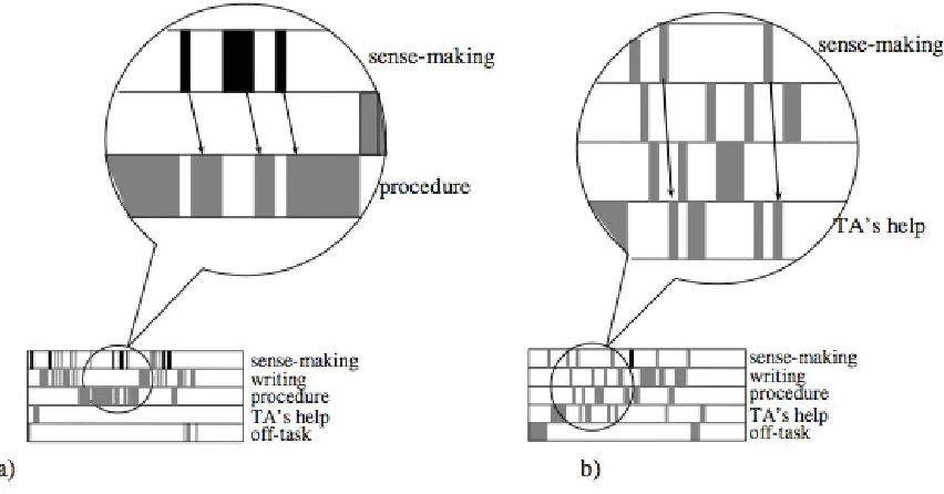
Figure 2.6 Temporal profile of sensemaking outcomes in a)ISLE labs where “a dis-cussion leads to a disdis-cussion and a conclusion” and b) non-design labs where “sensemaking leads to TA’s help with the TA answering and ex-plaining.”(Karelina et al, 2007) . . . 52
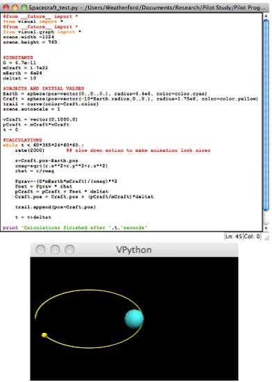
Figure 3.1 Program code and visual output for Spacecraft.py . . . 58
Figure 3.2 An excerpt of lines 3-17 of the Spacecraft.pyprogram . . . 60
Figure 3.3 Brian’s whiteboard prediction. . . 65
Figure 3.4 Alex’s whiteboard prediction. . . 67
Figure 3.5 Ana describing the effect of the force on the spacecraft with a momentum smaller than the momentum required to maintain a circular orbit. . . 72
Figure 4.1 The MWP code for the Earth-Spacecraft system. . . 81
Figure 4.2 The visual output for the Earth-Spacecraft MWP . . . 82
Figure 4.3 The program code and visual output for the three MWPs developed to be included in computational activities. The pink box lists the new lines of code students need to generate and add to the program such that the MWP predicts an appropriate behavior of the corresponding physical system. . . 85
Figure 4.4 Instructional tasks listed in sequence using a MWP. . . 87
Figure 4.5 Computer model of the QERL lab environment. The lab furniture in-cludes four tables, each accommodating three participants per table, a workstation and a whiteboard. . . 91
Figure 4.7 Screenshot of two frames from the same video file for a group working on the Spacecraft-Earth MWP activity. The webcam video feed is inlayed into an alternating feed between the over-the-head video and the recording of the monitor output. . . 98 Figure 4.8 On the left, the Spacecraft-Earth MWP program provided to the
par-ticipants. On the right, the same program with all blank lines of code removed and each line of code assigned a line number. . . 101 Figure 5.1 A Line-Number plot for Group G1 as the participants work on the
Spacecraft-Earth MWP activity. . . 114 Figure 5.2 Line Number plot for Eugene, Selma, and Beatriz as they study and
predict the MWP . . . 117 Figure 5.3 Line Number Plot for Roslyn, Estelle, and Roslyn as they study and
predict the MWP . . . 121 Figure 5.4 Yolanda’s whiteboard prediction. . . 122 Figure 5.5 Line Number Plot for Xavier, Howard, and Tina as they study and
pre-dict the MWP . . . 124 Figure 5.6 Line Number Plot for Dora, Lidia, and Norma as they study and predict
the MWP . . . 126 Figure 5.7 Line Number Plot for Ramon, Otis, Greg, and Fernanda as they study
and predict the MWP . . . 131 Figure 5.8 Line Number Plot for Paine, Zeke, and Frank as they study and predict
the MWP . . . 134 Figure 5.9 Paine’s position for the spacecraft relative to Earth. . . 136 Figure 5.10 Final prediction for the motion of the spacecraft traveling around the
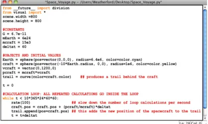
Earth. . . 138 Figure 5.11 Screen shots of the visual output running the Space Voyage MWP code
(a)when the visual output first becomes visible, (b) as the camera begins to zoom out to keep the objects in the field-of-view, and (c) some time later. . . 144 Figure 5.12 The Mass-Spring MWP code with line numbers added and blank lines
removed. . . 155 Figure 5.13 Visual output for the Mass-Spring MWP program before the mouse-click
(left picture) and after the mouse-click (right picture). . . 156 Figure 5.14 Line Number plot for Celia and Madeline as they study the program
code and draw a “prediction” on the whiteboard. . . 158 Figure 5.15 Madeline’s whiteboard prediction before running the program for a
sec-ond time. . . 160 Figure 5.16 Line Number plot for Isis, Estelle, and Frank as they study the program
code and draw a whiteboard prediction . . . 162 Figure 5.17 Isis drew predictions for the location of the ball (left), a larger prediction
Figure 5.18 Line Number plot for Ramon, Selma, and Dora as they study the program code and draw a whiteboard prediction. . . 166 Figure 5.19 Ramon’s prediction for the locations of the ceiling, ball, and spring. The
writing off to the right of the helix is “.26” . . . 167 Figure 5.20 Line Number plot for Lidia, Beatriz, and Otis as they study the program
code and draw a whiteboard prediction. . . 169 Figure 5.21 Whiteboard prediction for Lidia, Beatriz, and Otis. The text above the
line representing the ceiling is “h0,0,0i”, and the text besides the helix is “h0,−.3,0i” . . . 171 Figure 5.22 Line Number plot for Norma and Fernanda as they study the program
code and draw a whiteboard prediction. . . 173 Figure 5.23 Line Number plot for Yolanda, Xavier, and Zeke as they study the
pro-gram code and draw a whiteboard prediction. . . 176 Figure 5.24 Line Number plot for Max and Eugene as they study the program code
and draw a whiteboard prediction. . . 179 Figure 5.25 Rutherford Scattering MWP code provided for participants with line
numbers added and blank lines of code removed. . . 195 Figure 5.26 Visual output for the Rutherford Scattering MWP program at the
begin-ning of the simulation (left picture), as the alpha particle approached the gold nucleus traveling at a constant speed (middle), and after the alpha particle passes through the gold nucleus(right). . . 196 Figure 5.27 Line Number plot for Zeke, Isis, and Roslyn as they study the program
code and draw a whiteboard prediction. . . 197 Figure 5.28 Screenshot of Zeke drawing the path of the alpha particle moving towards
the gold particle(left), picks up marker and continues tip through the gold (middle), and returns to the trail to add an arrow at the location of the gold (right). . . 199 Figure 5.29 Line Number plot for Frank, Madeline, and Estelle as they study the
program code and draw a whiteboard prediction. . . 201 Figure 5.30 Line Number plot for Howard, Tina, and Xavier as they study the
pro-gram code and draw a whiteboard prediction. . . 204 Figure 5.31 Line Number plot for Celia, Paine, and Yolanda as they study the
pro-gram code and draw a whiteboard prediction. . . 208 Figure 5.32 Line Number plot for Otis, Selma, and Greg as they study the program
code and draw a whiteboard prediction. . . 212 Figure 5.33 Line Number plot for Eugene and Dora as they study the program code
and draw a whiteboard prediction. . . 216 Figure 5.34 Line Number plot for Max, Beatriz, and Lidia as they study the program
code and draw a whiteboard prediction. . . 218 Figure 5.35 Line Number plot for Ramon and Norma as they study the program code
and draw a whiteboard prediction. . . 221 Figure 6.1 Revised model for computational activities using a MWP as a result of
Chapter 1
Introduction
Computation offers physics education the possibility of examining complex, unidealized sys-tems which are out of reach of traditional analytical methods. By applying an algorithm consisting of the iterative application of physics principles, students can explore and predict the time-evolution behavior of two- and three-body systems interacting through gravitational or electrostatic forces and the dissipative effects of friction on falling or sliding objects such as springs. Both of these systems are commonly discussed in varying levels of detail in the in-troductory physics course, and a computational approach offers an open-ended time-evolution analysis of these more complex systems. Recognizing the usefulness of computation to offload the heavy iterative workload of an algorithmic approach to open-ended solutions, introductory and intermediate physics courses are integrating computation into their curriculums. There are two approaches to using computation in the introductory calculus-based physics curriculum: 1) provide students with simulations that model complex systems and the freedom to explore the effects of varying initial conditions on a system of interest, or 2) provide students with a programming environment in which they may build or alter a computational model to examine a complex system.
quan-tities and 2) provide a medium through which the open-ended application of physics principles are used to evolve a system’s dynamics. As such, students are asked to complete activities where they are tasked with building computational models. The hope is that by building computa-tional models which involve the application of fundamental physics principles, students gain a greater conceptual understanding of how a few fundamental principles can apply to a wide variety of systems.(Chabay & Sherwood, 2008) Prior research provides some evidence in sup-port of this endeavor in pictorial programming environments such as STELLA (e.g. Costanza, 1987) or spatial programming environments such as Boxer (e.g. diSessa & Abelson, 1986). This research is examined in greater detail in Chapter 2 of this dissertation.
It is an open question as to how students use their knowledge to interpret and apply physics principles across different programming environments. In Matter & Interactions, students use the VPython programming environment to build computational models. VPython is a 3D graphics module that provides Python programmers with access to a navigable 3D display and create animations with ease. VPython provides the option of importing graphics libraries to draw 3D objects within a virtual 3D window, or visual scene. Students have the freedom to control the visual attributes of these 3D objects by changing their default attributes in a text editing environment. Combined with the iterative application of physics principles, students can create time-evolving models of the positions of these 3D objects to produce simulations corresponding to analogous real-world behavior of interacting systems. Computational activities were developed to guide students through building a computational model and have been used in studio-style lab settings where students, working in collaborative groups of three, complete scaffolded tasks to achieve a valid and working program. These computational activities are based on research investigating the difficulties students have in creating a computational model from scratch, providing extra information to aid in the completion of the programming task when students most often need help (M.Kohlmyer, 2005).
Figure 1.1: Buffler’s model for computational activities in physics (Buffler et al, 2008, p.432).
Buffler et al.(2008) in Figure 1.1. Buffler shows the process to produce a computational model of the mathematical model which eventually runs to generate a visualization of the numerical output in the form of an animation. First, you start with a mathematical model for the system. From the mathematical model, one translates initial state variables and system of equations into programming syntax which iteratively calculates and updates the values of these state variables to produce a numerical output. With VPython, 3D objects are used to visualize these quantities to produce an animation of the numerical output at runtime. In Buffler’s computational activities, he asked his students to predict features of the dynamics of the system based on the mathematical model. Then, after the students translated the mathematical model into a computational model, he asked students to compare the prediction of the mathematical model to the visual output.
visual scene and an animation without receiving any error messages from the compiler. The intended goal of the computational activity was to provide students with experience generating a computational model based on the iterative use of fundamental physics principles and explore the model by changing initial values and observing the effects of these changes to the simulation in the navigable 3D visual output. That is, students focus on the programming task and not how the model generates a prediction for the evolution of a system of interest.
A pilot study was conducted to investigate further the difficulties students have completing tasks which focus on building the computational model in VPython. Students were recruited who completed the first semester of the Matter & Interactions course and therefore the com-putational activities included in the first semester. One major finding of the study, which is discussed further in Chapter 3, is that students who were capable of interpreting the individual lines of code in an example program had a difficult time thinking through how the program’s execution could display the events which unfolded in the visual scene. Student predictions of the visual output were mostly correct, including the effects of interactions between 3D objects and how the object’s motion would evolve in the simulation. However, it’s not clear that the predictions were a reflection of an interpretation of the program code or, alternatively, an ex-pectation of system behavior unrelated to thinking about how the program code evolves the
dynamics of the system. Investigating this question further provides an opportunity to add to the physics education literature on how students create an informed comprehension of system dynamics using evidence contained in an accessible computational model juxtaposed with their own conceptual understanding of physics quantities and principles. This led to the generation of a new type of computational activity which initially focuses on comprehension of program-ming code rather than generating programprogram-ming code. As a result, the instructional model for the computational activities is a modified version of Buffler’s Model (2008), and is presented in Figure 1.2. Before asking students to create program code, the activity begins with students interpreting a program that is incomplete, but still functional. The program is incomplete with regards to the computational model not including all the necessary physics calculations to generate an accurate prediction of the system. The program is functional in the sense that the program will produce a navigable 3D visual scene and an animation of the numerical so-lution generated by the computational model in its incomplete form. While students interpret the program, they are asked to generate a drawing to represent their prediction of what they might see happen in the visual scene or animation before they are allowed to run the program for the first time. Chapter 4 elaborates further on this new activity as well as the motivation behind asking students to interpret a program that isn’t finished. This dissertation explores the primary question underlying the interpretation of this new type of program:
How do students use their physics knowledge to make sense of
incom-plete, but functioning VPython programs?
Chapter 4 defines the characteristics of an incomplete, but functional program and provides three example activities, each incorporating a different program. Recordings of participants in a research laboratory environment are used to serve as the data to answer the research question. Chapter 4 continues to report the details the experimental study and its design goals as well as the techniques used in analysis of the data generated during the study. Chapter 5 presents the results from the analysis of the data, comparing student groups to one another as they work on the instructional tasks. Chapter 6 concludes the study with a discussion of what was learned, what new knowledge is now part of the research literature, further implications for instructional design of computational activities, and the avenues for future research to examine how to use computation to enhance the conceptual understanding of physics.
But first, this chapter will detail the terminology used in this dissertation when referring to the fundamental physics principles or programming concepts.
1.1
Terminology
Matter & Interactions emphasizes the use of a small set of fundamental principles which are valid for all systems. The Momentum Principle is particularly useful in building computational models due to the vector nature of the physics quantities which, combined with the Position Update formula, provides enough information to evolve the spatial attributes of 3D objects in a 3D visual scene. Eqn (1.1) shows the algebraic representation of the Momentum Principle in its update form. The update form of the Momentum Principle is useful as an interpretation of how the new value of the momentum of the system equals the previous value at the beginning of an interval plus a quantity that quantifies the nature of the interaction between it and its surroundings.
~
pcraft=pcraft+Fnet*deltat (1.2)
The computational analog, or Eqn (1.2) shows how this algebraic equation might appear in a computational model. The interpretation of Eqn (1.2) is somewhat different from its algebraic interpretation.(Sherin, 1996) Each of these variable names represents stored values that were initially given some value. If these variables represent vector quantities for the momentum and net force on a spacecraft, and thedeltatrepresents the interval of time during which the force is approximated as a constant value, then this line of code represents the algebraic form of the Momentum Principle with the function of updating a value store in system memory which represents the value for the momentum of the spacecraft.
The position update formula computes the new position of a system of interest due to the average velocity over a time interval. Eqn (1.3) shows the algebraic representation of the Position Update formula. The computational analog to this formula is shown in Eqn (1.4) and updates the attributes of the 3D object named craft based on the current value for the momentum of the craft, the mass of the craft, and the interval over which the momentum is approximated as a constant value. Using the updated value of the momentum instead of the average of the old and updated values produces an algorithm which is stable.(Timberlake & Hasbun, 2008)
~rfinal=~rinitial+
~ pavg
m ∆t (1.3)
craft.pos=craft.pos+pcraft/mcraft*deltat (1.4)
defined on a 3D space.
Esys,final=Esys,initial+ ∆Esurroundings (1.5)
Chapter 2
Literature Review
2.1
Introduction
This literature review is segmented into three sections, each discussing a relevant sector of literature relating to this research project:
2.2 Computation in Introductory Physics
2.3 Program Comprehension & Reading Comprehension
2.4 Sensemaking in Physics Education Research
Section 2.3 analyzes the research by cognitive psychologists to develop a model of the mind using a computational metaphor by studying how programmers complete programming tasks. For this dissertation, the comprehension of computer programs is of particular interest. The section analyzes the program comprehension models for similarities to the primary functions of reading comprehension, as identified by Palinscar & Brown (1984).
Section 2.4 examines the physics education research literature on sensemaking. Recently, researchers have focused their interest on how students work towards identifying goals and complete tasks during an instructional activity. This section reports how these researchers identify sensemaking and distinguish sensemaking from other forms of student activity, and how this identification is a useful measure of student engagement.
2.2
Computation in Introductory Physics
This section begins by exploring a fundamental shift in instructional goals by computer scien-tists.
2.2.1 Computational Thinking
Abelson & Sussman (1984), in the preface of their procedural textbook pointed to the computer revolution as a “revolution in the way we think and express what we think.” They referred to this metacognitive analysis as a procedural epistemology, “the study of the structure of knowledge from an imperative point of view.” Meaning, just as mathematics provides a framework for “what is”, computation provides a framework for “how to” (Abelson & Sussman, 1984).
algorithmic thinking involves the ability to analyze problems from an algorithmic point of view, apply existing algorithms for their solution, develop new algorithms for unique problem situ-ations, implement the solution and finally run and test the solution on a computer (Syslo & Kwiatkowska, 2008).
Jeanette Wing’s (2006) essay argues that computational thinking is a fundamental skill, useful in applications outside of computer science. With the introduction of object-oriented languages, Wing elevates the role of creating abstractions and layers of abstractions with the knowledge of appropriate algorithms to deploy as a way to think like computer scientists. Wing argues that computational thinking in analytical sciences extends the domain of creative problem solving. By providing opportunities to ask questions otherwise unimaginable, compu-tational methods extends the reach of analytical sciences to produce simulations which evolve analytical models.
Qualities of computational thinking includes: 1) thinking at multiple levels of abstraction, 2) having the freedom to construct virtual worlds and engineer systems beyond the physi-cal world, 3) using imagination to tackle inconceivable problems through reduction and task analysis, 4) using computational concepts to solve everyday problems and manage daily lives (Wing, 2006). Note that computational thinking is more than knowledge about different types of algorithms. Computational thinking includes initiating a range of mental tools and con-cepts (abstraction, induction, heuristics) applied to a specific problem to develop a process to efficiently and approximately makes the problem tractable in order to compute a solution.
2.2.2 21st Century Curriculum Re-Design
the education research literature has explored the roles computation can play in a formal ed-ucation setting to display abstract concepts and provide the opportunity for students to build computational models. Physics education researchers have explored the use of computation as a tool to enhance qualitative conceptual learning through interactive simulations (e.g. Perkins et al., 2006; Linn, Lee, Tinker, Husic, & Chiu, 2006; deJong, 2006; Christian & Belloni, 2000; Singh, Belloni, & Christian, 2006). Others use programming languages as a representational language in introductory physics courses to enhance the conceptual learning goals of the cur-riculum (e.g. E. Redish & Wilson, 1993; Chabay & Sherwood, 2004, 2008; Buffler et al., 2008). Finally, others explicitly teach computational methods in parallel with introductory and upper level physics courses for majors (e.g. Landau, 2006; McIntyre, Tate, & Manogue, 2008; Roos, 2006; Taylor & King, 2006). Since the focus of this dissertation is on how students use physics to understand computational models, this section will restrict its breadth to how researchers have studied and used computer modeling environments in educational settings.
2.2.3 Computer-Based Modeling Environments
This section explores the different types of microworld environments researchers have used to explore how students apply physics to such environments.
M.U.P.P.E.T.
Pascal on Macintoshes, or Turbo Pascal on PC). The curriculum augmented the traditional physics sequence to include more realistic problems and situations beyond the limitations of students’ formal mathematical training. The focus of the project was to expose students to a class of physics problems designed to analyze real systems using a discrete form of fundamental principles. Through discrete representations of physical laws combined with the added power of computation, the introduction of physically important ideas may occur at an earlier stage than otherwise possible. An early introduction to these ideas promotes a hierarchical ordering of material to help students decide on “the relative strengths of the various concepts, principles, and techniques presented in the curriculum.” (MacDonald, Redish, & Wilson, 1988)
The M.U.P.P.E.T. project followed three guiding principles of design: 1) rethink the cur-riculum entirely assuming the availability of the computer (what can we teach that we couldn’t teach before?), 2) the computer should not replace the teacher, textbook, or the laboratory, and 3) the student should run the computer, rather than the other way around. (MacDonald et al., 1988)
Redish(1993) reported on the capabilities of the M.U.P.P.E.T. environment to provide op-portunities for students to complete research projects of interest, somewhat connected to the topics contained in the introductory physics course. The goal of these projects was to provide an open-ended investigation fashioning itself on the methods and techniques of doing science. Prior to M.U.P.P.E.T., Redish reported that student work lacked the desired characteristics of scientific research. Using M.U.P.P.E.T., two-thirds of the students produced projects Redish considers “valuable and interesting.”
range of physics problems, and 3)will the computational course shift attitudes towards physics. The computational activities took the form of additional work to the normal curriculum on quantum mechanics for research trials 1 and 2. After the first and second trials, the authors concluded 1) “students do not need to be able to program before handling these materials” and 2) “the students’ understanding of a number of traditional subjects was significantly improved by adding computer modeling problems as shown in a comparison of the students in the test and traditional groups on traditional tests.” Johnson & McPhedran attributed this performance gain to student exposure to additional physical situations beyond the limitations of analytical cases.
STELLA
STELLA (Structural Thinking Experimental Learning Laboratory with Animation)1 provides programmers a method to represent state variables and their relationships as a collection of iconic structures in a concept-map-like environment. STELLA was designed to minimize the demands on any programming and mathematical skills. (Costanza, 1987) Figure 2.3 provides an example of how this representation describes the quantitative relationships between accel-eration, velocity, and position. (Schecker, 1993) After defining initial conditions and form of graphical representation to display, STELLA extracts the differential equations from the map and evolves the system. STELLA provides a collection of visual icons for creating structural relationships, which define the dynamics of a system.
The design of STELLA allows students to focus on the qualitative relationships between quantities and how these quantities change values through time. It is argued to serve as an advantageous environment to deal with conceptual relations over mathematical formalism. Ad-ditionally, Chi (1981) shows, from her expert-novice research, that experts often tend to first use a qualitative approach when solving problems.
1
One drawback of STELLA is the limited set of objects and relations that can be expressed in the environment. This limits the conceptual tools available to students in building models to the following: 1)stocks, or representations of things that build up over time, 2)flows, allows the control of stocks, 3) converters to generate outside influences and graphical relationships, and 4) connectors, to show the direction of proposed relationships. In order to use STELLA, students must conceptualize systems using these productions. Students who have alternative models of relationships may have trouble constructing a complete and coherent model with the provided tools. (Penner, 2000) Further, any evaluation of the STELLA model from graphical outputs may not reflect the student’s conceptual thinking.
Schecker (1993) developed an empirical study to investigate how students use STELLA to study motion. His goal was to help students realize that the same qualitative model may be used to explore a wide range of dynamical systems. That is, students can model a different phenomena by changing the forces involved for each system, without altering the top-level process. Figure 2.4 shows the STELLA model for a meteor falling in the atmosphere. After completing an experimental semi-quantitative activity to determine the effects of velocity, air density, and cross-sectional area on friction acting on paper cones, students took 20 minutes to create a STELLA model of a parachutists. Finally, students modified this program to extend the model to an asteroid falling through the atmosphere. Schecker claims “by working on complex examples for which standard calculations fail, students realize that it is essential to have a qualitative understanding of physical structures - these can be applied universally, special equations cannot.”
Table 2.1: Table II from Hogan and Thomas(2001).
Phases of modeling More productive approaches Less productive approaches Model construction Thinking about system behavior
and the burden of interpreting model output while specifying model parts and relationship
Tending to focus on representing real system ingredients without an-ticipating system behavior when constructing model parts and rela-tionships
Model quantification Taking a budget view of all in-puts and outputs, and think-ing about continuous relationships, when choosing values and building equations for model parts
Considering only one variable or set of equations at a time, instead of thinking about the dynamic inter-action of all model quantities over time, and using constant to repre-sent varying quantities
Model interpretation Using output to explore the rela-tionship between how a model func-tions and how it is structured and specified
Failing to investigate carefully why a model yielded particular output
Model revision Using output to guide a range of types of revisions, including model parts, relationships, and quantities
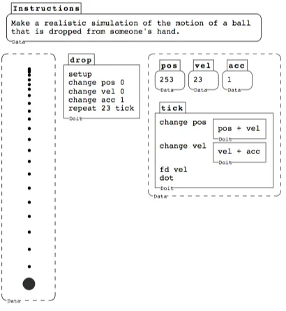
Boxer
Boxer2 takes its name from its design, where all computational objects within the program
are represented by boxes containing text. (diSessa & Abelson, 1986) The environment takes advantage of the computer monitor as a valid representational tool and uses it as an opportunity to create a 2D expressive environment. This environment was designed with two principles in mind - spatial metaphor and naive realism. Spatial metaphor refers to the relative location of programming objects. For example, smaller boxes can be nested into larger boxes, representing hierarchical structures. While a cursor is inside of a box, information pertaining to the box is accessed and can be treated as a separate environment. Figure 2.5 details the nested nature of boxes to create a hierarchical loop structure for repetitive calculations, the current values for the variables representing position, velocity, and acceleration, and a display of the printed position of the object after each repetition of the tick procedure. Naive realism refers to the belief by the programmer of immersion into the microworld. The monitor displays all the information pertaining to the environment. For example, creating a variable box will display the current value of the variable. Altering the value in the box will alter the variable value in the compiler. If the program alters the value in response to computing an algorithm, the text box displaying the variable’s value also changes. The action of creating a variable also provides a spatial location for the state of the variable at any time.
Boxer is an offshoot of Logo, a programming language designed to challenge students’ think-ing about a wide range of phenomena.(Papert, 1980) The design of Logo mimics how people conversationally describe movement and thinking about the world. By using commands such as forward andbackward, Papert hoped students would use their prior knowledge about movement to create a program to control the actions of an icon called a “turtle.” (1980)
Although Logo was developed explicitly for educational purposes in the late 1960s, it
pre-2
ceded any pragmatic usefulness by 15 years. The cost of a computer to run Logo at the time of its development was well over a million dollars, and through the 1970s as the cost of computers came down, researchers refined the Logo language and ran extensive pilot studies with teachers and students. (diSessa, Abelson, & Ploger, 1991) Since the early 1980s educators have taken to the environment with research into its effectiveness as an introductory programming environ-ment being investigated in over 300 instances since 19813. Logo has recently been reincarnated (Mindstorms) as a language for robotics education in the LEGO community and has been used in summer camps to promote scientific inquiry skills and the development of conceptual physics knowledge through robotics.(Williams, Ma, Prejean, Ford, & Lai, 2008)
Penner (2000) notes in a review of research investigating the use of programmable media in education, that the focus of research involving students using Logo has mainly been within the domain of mathematics. Researchers have been interested in how students create procedures using operators to instruct the turtle to draw geometric shapes. And during the 80s, over 90% of the research focused on “how the use of Logo affected the development of general problem-solving skills, critical thinking, collaborative learning, or metacognitive awareness” (Penner, 2000) and not on modeling physical phenomena. Kynigos (1995) investigated a phenomena first observed by diSessa where 12 year-old students who have had experience drawing geometric shapes in Logo have a very difficult time transitioning to programming a turtle that is responsive to Newtonian physics. Kynigos attributes the difficulties to conceptions of processes of change of time, which is not relevant when drawing two adjacent sides of a square, but is relevant when programming a turtle to turn 90 degrees.
DiSessa(1982) reports in a study of elementary school students (11- 12 years old) and an undergraduate student (Jane) of uniform and consistent strategies to kick a moving Logo turtle in a direction towards the target, with the expectation that the turtle will move in the direction of the push. While using commands R, L to turn the direction a turtle faces by 30 degrees,
3A cursory search for “Logo” in ERIC for published papers specifically investigating the use of Logo in
and K to give a turtle some kick/velocity along the direction of the facing turtle, students were asked to answer the question: “What kick (vector) should I provide to turn a corner.” The program provided an initial position of the turtle and the target such that the turtle could not face the target. The turtle’s initial velocity was zero. DiSessa provides the full 24-game results for Jane, an undergraduate student taking physics. Her Aristotelian strategy was only effective when she decided to provide an anti-kick to the turtle to bring it to rest followed by a rotation of the turtle and subsequent kick to reach the target. DiSessa notes this as a strategy related to that is commonly used in sports (soccer, hockey). Jane’s strategies were remarkably similar to strategies used by elementary school students. Further, diSessa notes that Jane “did not, indeed for a time could not, relate the task to all the classroom physics she had had.” (1982, p.59) DiSessa speculated that Jane has two types of representational schemes – one which is quite formal for deploying her physics knowledge (which she demonstrated having no fault in using vectors) and one intuitive, loosely organized schema motivated by a situational cue.
The Boxer Group at Berkeley investigated the use of Boxer in a high school physics course taught in 1991. (Sherin, diSessa, & Hammer, 1993) The 15 week long class was split into two parts: the first five weeks were devoted to Boxer programming and the remaining 10 were devoted to introductory physics. Activities during the Boxer portion of the class introduced students to the fundamentals of Boxer. The following 10 week physics course was designed around the creation of five core programs by student design: 1) A dropped ball from rest, 2) a ball dropped from a moving platform, 3) a puck sliding on frictionless surface, 4) a ball thrown in an arc, and 5) a chair pushed at constant speed across a floor. The design activity was facilitated by a teacher-led discussion including all eight students in the class. The teacher wrote syntax and asked follow-up questions of the students clarifying which elements were needed in the program for the turtle to complete a specific task.
specifically on an episode where students discussed how to write a modified procedure for the turtle graphic to turn right. The students discussion provided evidence of a pattern the researchers noticed as occurring often in these lab sessions: “students modified the program procedure, and then ran the program in their heads to see how it worked.” (Sherin et al., 1993) Sherin attributed this behavior as a method for students within the group to clarify how Boxer commands were interpreted by the program, and if they match the actions required by the design task.
After analyzing the teacher-led design activities, Sherin explains how the structure of the tasks lead to a deeper understanding of physical phenomena without asking the students to analyze anything. Sherin argues that the task to analyze a physical phenomena by novice physics students is an ill-defined task, as it requires “a knowledge of particular reasoning strategies, appropriate approximations, and idealizations, as well as a knowledge of fruitful areas of focus.” Rather, Sherin uses these programming episodes to justify a task modeled on how students learn as children – by actions that follow the design, implement, and modify sequence.(Sherin et al., 1993)
Sherin argues the design activity supported a necessary level of abstraction, which was nat-urally initiated by the students. For example, the students did not worry about air resistance when modeling a moving cart. The teacher had to press students on air resistance when chal-lenging the accuracy of their working program. Sherin notes that idealizations such as ignoring air resistance is disingenuous when attempting to understand the real world; however such sim-plifications are adequate and perhaps necessary when trying to portray the real world.(Sherin et al., 1993)
com-mand, and finally comparing this action to the desired goal. The execution of a command must be explicit and free of errors. Boxer contains a limited set of objects which serves to constrain the available set of programming options. Sherin argues that this limitation helps constrain student inquiry to how to use the available features in a physically meaningful way. Students benefit by focusing on the physics concepts rather than how different Boxer objects manipulate the turtle. (Sherin et al., 1993)
One feature of Boxer’s box structure that lends itself to investigations of how students perceive discrete motion is how Boxer represents processes with the tick model. The tick box repeats all lines of code for one unit of change in time (∆t). Boxer allows students to move within the tick procedure to view the effects of each line of code on the turtle and the values inside the variable boxes (Figure 2.5). All of the programs created by students in Sherin’s thesis work used this tick box, which provided Sherin the opportunity to observe carefully how students interpret the tick procedure. He noted an exchange between two students who tried to determine if the order of the equations within the tick box mattered, with one student interpreting the tick box as evaluating each line separately occurring through time rather than a series of actions that occur once for each ∆t. (Sherin, 2001)
There exists no evidence from literature or a public presence on the web of further devel-opment of Boxer4. The latest version of Boxer has not kept up with the popular operating systems and hardware of today’s modern personal computers.
VPython
The development of a 3D graphics library for Python by the VPython development team5
pro-vided support for scientific visualization (Scherer, Dubois, & Sherwood, 2000) with a computer language that had already been argued as a suitable language for inexperienced programmers. (Conway, 1997) Ruth Chabay and Bruce Sherwood reported on their experiences introducing VPython to introductory calculus-based physics course at Carnegie Mellon University, offering an anecdote where 75% of students in a second-semester physics course were able to recall how to program a proton to move due to its interaction with an ambient electric field in approxi-mately 15 minutes or less.(Chabay & Sherwood, 2000) Further development on computational activities continued and reported as a full-fledged component of the Modern Mechanics (Chabay & Sherwood, 2004) and Electric & Magnetic Interactions (Chabay & Sherwood, 2006) and
fur-4
http://dewey.soe.berkeley.edu/boxer/papers.html
ther justified as a valid component of the introductory calculus-based physics course (Chabay & Sherwood, 2008).
The VPython programming environment is used to support the central goal of the Matter & Interactions curriculum: to develop a conceptual understanding of fundamental principles. One observable benchmark indicator of progress towards this central goal is for students to spontaneously use fundamental principles to analyze non-trivial systems. Research in physics problem solving reveals that novice students have difficulty thinking about physics in this fashion. A study by Chi et al.(1981) reveals differences between expert and novices during a sorting task for a collection of physics problem statements. Experts sort physics problems according to major fundamental principles that would be used in their solutions while novices sort physics problems according to the features of the system and the problem statement.
principles. Further, empirical anecdotes from TAs indicate the state of students’ epistemolog-ical focus is characterized by the intensive goal of generating a working program and not on building a greater conceptual understanding.
Buffler et. al.(2008) provide similar accounts of honors physics students’ epistemological goals during computational activities. Buffler et al.(2008) detailed a model for designing com-putational tasks which closely models the methods used by comcom-putational physicists to build computational models of physical systems. The sequence of the activity begins with formulating a mathematical model using fundamental physics principles that constrains the time-evolution for a system, making predictions of the motion of objects based on the mathematical model, translating the mathematical model into a computational model, and reflecting on the numeri-cal solution by comparing the visualization to the initial predictions of the mathematinumeri-cal model. This sequence, and the relationship between each component Buffler et al’s(2008) conceptual model is shown in Figure 1.1. The model explicitly brings together all representations of a physical system. The activities assume students understand these representations serving as coherent and valid abstractions of the physical system and is cognizant of these limitations when applying to real-world phenomena. Further, Buffler’s model does not include any reflection on relating the conceptual models, realized through the computational medium, to the real-world phenomena.
information, however were told to expect the problems to be difficult.
None of the students from the traditional physics sections resorted to writing a computer program, or considered the use of a computer as a valid means to a solution. Kohlmyer re-sponded by noting that this finding is expected, as traditional students are not taught iteration or use a programming tool during their formal instruction. Several traditional students at-tempted to develop integrals, recognizing the challenge of analytically solving equations of motion involving a time-dependent acceleration.
Only two of five M&I students chose to use the computer and generate programs to model the problem. Kohlmyer suggests the interaction of an unfamiliar, novel task may explain the actions of students rather than the ability of students to complete an iterative calculation. According to Kohlmyer, student apprehension of computer programing may be alleviated by the introduction of similar types of tasks in the M&I course. Providing an opportunity for students to make a decision on whether to complete a problem by analytical methods or computational modeling may improve student success on this sort of task.
Kohlmyer’s second experiment investigated the difficulties students have with generating VPython programs and the effects of a tutorial-style intervention on these difficulties. Results reported student difficulties with physics concepts rather than with programming syntax. Fur-ther, the transcriptions detail how difficult the problem-solving task of generating a computer program for a simplistic two-body system can be for novice students. Kohlmyer adapted instruc-tion to account for these difficulties by minimizing the amount of new informainstruc-tion presented to students in any single computational activity, and reduce the number of complex tasks by providing some of the missing information, such as initial conditions.
Coding the major interventions by its conceptual purpose reveals the frequency with which these concepts impede completion of the programming task. Since some of these difficulties were not intended to be stumbling blocks in the activity, instruction was redesigned to provide additional help in completing the programming tasks. The modified instructional sequence includes an additional computational activity where students are guided through a sequence of calculations for the gravitational force of a static object at several locations in space. The next activity is designed to allow students to use the gravitational force calculations to model a moving and interacting spacecraft with the Earth. Due to the difficulties students were having choosing an appropriate initial velocity of the spacecraft to produce a circular orbit in Kohlmyer’s second experiment, the modified instructional sequence provides the initial velocity and position of the spacecraft which will produce an elliptical orbit. The student task is to decide which of the gravitational force calculations are to go inside the loop structure, code these calculations into understandable computer syntax, and include calculations to update the momentum and position of the spacecraft. The influence of the spacecraft on the Earth is approximated as insignificant in this program.
2.2.4 Multiple Representations
Using VPython provides the opportunity to connect different types of representations as coherent and valid depictions of a computational model. Specifically, the visualization of ab-stract physics quantities using 3D objects in pseudo-time should help build an understanding of the fundamental principles of physics. In trying to understand how to make sense of each student’s success in reaching the goals of the curriculum through activities designed to promote and evaluate these goals, researchers have found it helpful to think about how representations differ along cognitive dimensions.
Animations
Animations serving in a multiple representational regime is merely a collection of diagrams given a temporal sequence. Since the temporal nature of any two diagrams in the sequence is added information, one might hypothesize that this added information may be more useful to learners as it both increases “processability” as well as limits the need for the abstract transformations of elements in a static display. In a review of previous research investigating the perceived advantages of animated diagrams over multiple static diagrams Tversky (2002) criticizes conclusions that animations have a cognitive advantage over diagrams, due to hidden non-temporal features that make the animations superior. That is, the animations used in comparisons either contained extra information (e.g, Park & Gittelmann, 1992; Rieber, 1990), or different procedures such as added interactivity (Kieras, 1992), that were not included in the static diagrams. Further Byrne, Catrambone, and Stasko (1999) found no advantage of animations over providing static diagrams and asking for student predictions, in understanding of computer algorithms. And, conditions that compare the effects of both animation and prediction to conditions without either show no significant benefits of either treatment.(Hegarty, Quilici, Narayanan, Holmquist, & Moreno, 1999)
saxo-phone) by explaining and segmenting the event into units, making decisions when “one unit ends and one unit begins.” Analysis reveals that the population simultaneously keep track of physical changes, goals and plans, causes and effects, and actions and objects. Segmenting includes a hierarchical structure of recursive activities (when valid) and verbal explanations of segments reflect the physical changes of objects towards the goal-state. This study is relevant to how one perceives animations, particularly for animations showing processes that can be de-scribed such as in circuits, pulley systems, or traveling across town. Zacks et. al. (2001) points to this research and others in claiming that even when motion is continuous, people conceive of it in discrete steps, similar to the key frames that would be present in multiple static diagrams of the event.
An open question is how animations that lack a goal-oriented focus are perceived into discrete events, the amount of abstraction inherent in these discrete events, and if these discrete events contain references to mechanism or merely descriptive of the motion characteristics of the animated objects.
Different functions of multiple representations
In earlier work, Ainsworth(1999) synthesizes research in multiple representations to build a taxonomy of how multiple representations are used to “maximize learning outcomes.” The tax-onomy segments all uses of multiple representations into three separate functions: 1) to support complementary cognitive processes, 2) to constrain interpretations across multiple representa-tions (where one representation acts to constrain the interpretation of another), and 3) to aid in constructing a deeper understanding.
Constructing multiple representations
Cox(1999) reviews the research literature investigating how constructing multiple representa-tions may aid in problem solving. Cox characterizes the task of constructing a representation as a process that involves students “examining their own ideas, re-order information, trans-late information from one modality to another (re-represent), and keep track of their progress through the problem.”(1999) Further, externalizing information into a representation may act to flesh out specific mental models used to visualize a particular problem, useful where problem solving is too difficult to complete internally. The underlying mechanism is the role of exter-nalization serving as a go-between in the transfer and storage of information among cognitive sub-systems as described by dual-coding theory. Wilkin (1997) reports in a study on the links between students creating a diagram and their self-explanations, that diagrams contribute to inaccurate self-explanations and concludes that the self-explanation effect may only apply to strong students. However, in Wilkin’s study, low performing students were encouraged to use a diagram system that they did not understand or find helpful in the same way the diagram was created and used during the self-explanations of high performing students.(Cox, 1999)
In his own work, Cox investigated any differences in the models of reasoning used by stu-dents who select, construct, evaluate one’s own representations or use pre-fabricated represen-tations from a textbook. Cox specifically investigated how one externalizes the representation, including any errors made in the representation’s construction, and the interpretation of the representation.
Cox (1999) , in his summary, explores the different possible uses of constructing multiple representations as an aid in problem solving. Cox’s list is filtered through the aims of this literature review, and include ways in which constructing multiple representations may be used via:
• directing attention
• providing perceptual assistance
• the self-expanation effect
• facilitating the inference of motion (mental animation)
• refining and disambiguating mental images
Mechanistic reasoning and multiple representations
To achieve the conceptual goals of the M&I course, students must see physics as a collection of a limited set of fundamental principles, through which one builds an understanding of systems and the evolution of the dynamics through time. As characterized by Russ, (2008) this type of reasoning addresses mechanism as a basis for scientific explanations, which include causal relationships between principles and observation, rejecting descriptions of objects/processes by their function or intent (Carey, 1995), searching for an underlying relevant structure (Chin & Brown, 2000), all which is constrained by the framework of previous experiences in the real-world (diSessa, 1993).
Identifying the organization of entities (spatial relations between entities), 7) Chaining: Back-ward and forBack-ward (claims about what might have brought about the entities current state, or its state in the future).
Russ (2008) applied this coding scheme as an analysis of student discourse for first-grade students to determine the quality of students’ mechanistic reasoning engaged during the in-teractions between a teacher and her students. Russ provides episodes from a transcript and analyzes the quantity of each code, deeming episodes with prolonged statements at the top of the hierarchy as episodes with strong evidence of mechanistic reasoning. Further, Russ in-vestigates the discriminatory power of the scheme to recognize transitions within an episode, noting that high-level codes tend to cluster. Transitions to higher-levels were either instigated by students or the teacher. Russ notes that transitions to level 7 all came from levels 3,4, and 5, suggesting that these levels provide the necessary building blocks to determine new mechanisms to consider.
2.3
Program Comprehension
2.3.1 Introduction
Cognitive psychologists focused their research efforts of modeling the mind as metaphorical computer during the 1980s and well into the 90s. As such, much of the research by those who adopt this metaphor studied programmers in how they generate and comprehend computer programs. Cognitive psychologists explored the difference between expert and novice program-mers in how they plan, generate, and debug programs in order to build models of problem solving and program comprehension. The first half of this section explores these findings in terms of how expert and novice programmers comprehend novel programs. The second half of this section investigates parallels between program comprehension and reading comprehension, specifically how one designs instructional tasks to improve reading comprehension and explores possible ways in which these tasks might improve program comprehension.
2.3.2 Cognition and Comprehension
Introduction