The diffusion equation method of global optimization is a mean field approximation to simulated annealing

The Diffusion Equation Method of

Global Optimization is a Mean Field

Approximation to Simulated

Annealing

Griff L. Bilbro

Center for Communications

and

Signal Processing

Department Electrical

and

Computer Engineering

North Carolina State University

The Diffusion Equation Method of Global

Optimization is a Mean Field

Approximation to Simulated Annealing

Griff L. Bilbro

Abstract

We show that the diffusion equation methodof global minimization of Kostrowicki and Piela is equivalent to mean field annealing, a previously reported deterministic approximation to

the usual simulated annealing algorithm. We derive the mean field approximation. We show

how to apply it to real-valued problems and present the results for high dimensional image

1

Introduction

Recently in this journal, Kostrowicki and Piela[7] reported successful applications of their

diffusion equation method to global minimization of low dimensional standard test problems

in the Goldstein-Price, Hartman, Shekel, and Griewank families. In earlier work we[l, 5, 2]

introduced mean field annealing and showed it to be a powerful and simple approach to a

variety of difficult optimization problems. Mean field annealing is a simple deterministic

approximation to simulated annealing.

In this paper we show that the algorithm of Kostrowicki and Piela is equivalent to mean

field annealing. Their "Fourier-Poisson formula" is the mean field condition for

approximat-ing real-valued systems. Their "reversapproximat-ing procedure" in time is equivalent to the gradual

reduction of temperature of simulated annealing. Kostrowicki and Piela have shown that

the approach is useful for low-dimensional problems. We will show that mean field annealing

is equally useful for high dimensional image optimization problems involving thousands of

real variables. We also show that mean field annealing applies equally well to

combinato-rial optimization

(e.g.

the traveling salesman problem), which it converts to more tractable

nonlinear optimization problems.

In Section 2 we will review the features of simulated annealing that are relevant to the

from information-theoretic considerations even though it it usually obtained with the tools

of statistical rnechanicsjl ,5, 2]. We will show in Section 4 how the mean field approximation

can be applied to both discrete-valued problems and real-valued problems. The formulation

for real-valued problems will be shown to coincide with Kostrowicki and Piela's diffusion

equation method. In Section 5 we will present results for a class of image processing problems

involving many more variables than Kostrowicki and Piela considered.

2

Simulated Annealing

In simulated annealing, minimization is reformulated as a stochastic sampling problem.

In-stead of minimizing U(

s)

with respect to 8 ESC RN, the associated Gibbs distribution

1

P[s]

=

Z

exp(

-U[s]jT)

is maximized. Here the normalization in the domairr' S

z

=

f

ds

N exp(

-U[s]jT)

(1)

(2)

depends on

T

only. The variable

T

is artificially introduced to create a family of distributions

that emphasize maxima at lowT. Since the exponential function is monotonically increasing,

finding the mode of P at any T is logically identical to finding the minimum of U.

3When the domain 5 is discrete, the integral is replaced by a sum, but in this article we are concerned

The two formulations differ practically, however, because the sampling formulation admits

the powerful Metropolis sampling procedure[9] which can efficiently produce instances of 8

that are statistically distributed according to Equation 1. At low enough

T,

every sample

s is practically the global minimizer. This approach feasibly efficient only

if

the sampling

is begun at a high

T

and continued as the temperature is gradually reduced, a procedure

called Simulated Annealing by Kirkpatrick, et al., who introduced it[6].

3

Mean Field Approximation

In earlier work we[l, 5, 2] showed that simulated annealing could be accelerated with the

mean field approximation. In this approach the important structure of

P

is approximated

with a more convenient distribution

Po

for a sequence of falling values of

T.

In this section

we provide an information-theoretic procedure for studying a given difficult P using an

es-sentially arbitrary easy

Po

by minimizing the entropy of

Po

relative to P, or equivalently, the

cross-entropy or Kullback-Leibler[8] distance between

Po

and P. This information-theoretic

procedure leads to our previously successful approach based on the theoretical tools of

sta-tistical physics.

Assume we have another positive but otherwise arbitrary distribution

Po

[s, m].

It is

some vector

rn,

We rewri te

Po

1

Pols,

m]

=

Zo

exp(

-Uo[s, ml/T),

where

Zo

==

J

ds

exp(

-Uo[s, m]/T)

which in general depends on m through

_Uo.

The entropy of

Po

relative to

P

is

J

Po[s,m]

R

=

dsPo[s,

m]

In

P[s]

,

(3)

(4)

where we have suppressed the dependence of R on the vector of adjustable parameters m.

Using Equations 1 and 3, we rewrite Equation 4 as

R

==

J

ds

exp(

-Uo/T) (-Uo/T

-In

z,

+

U/T

+

In

Z).

Zo

(5)

We define the average with respect to

Po

of a function </J[s] as (</J)

==

Jds</>exp(-Uo/T)/Zo

and obtain

1

R

==

--(Uo - U) -InZo

+

InZ.

T

We define

F

_o

== -

TIn

Zo

and

F

== -

TIn

Z

and obtain

1

R

==

-(Fo - F

+

(U - Uo) ),

T

(6)

(7)

It is known[8] that

R[m]

2:

0 with equality holding if and only if

Po

==

P.

Here

T

is also

positive so that

which is the basis of our mean field approximations to discrete, continuous, and even problems

with both discrete and continuous variables.

The mean field approximation is obtained by minimizing Equation 7 with respect to m to

find the tightest bound in Equation 8; mean field annealing involves tracking the minimum

from high to low values of

T[lO].

In the case of discrete s, as in graph coloring or binary

image restoration[

4]

it is useful to choose

(9)

but in the present context of problems with continuous s, the simplest useful choice[5, 2] is

(10)

In either case the m., are real.

4

Mean Field Annealing

Mean Field Annealing (MFA) is based on Simulated Annealing (SA) and derives its power

and generality from that popular optimization procedure. MFA differs from SA by

analyt-ically approximating the relevant Gibbs distribution rather than stochastanalyt-ically simulating

it. SA works by gradually cooling an on-going stochastic simulation of a Gibbs distribution.

can be cooled in the same way to produce a Mean Field Annealing (MFA) algorithm. Many

SA algorithms can be converted to analogous MFA algorithms that run in 1/50 the time

required by the SA version[11, 1, 5,

2].

However because it is an approximation, MFA does

not inherit any guarantee of convergence even when the analogous SA does converge.

4.1

Approximation of Systems of Discrete Variables

For combinatorial problems, the domain S

==

{O,

l}N is discrete and each solution might be

represented as a vector 81,82, ... ,8N ones and zeros. A typical objective function might be

U[

CIa] - - '"'" lu- L...J 1s. -1 '""'V"8'8'L...J 13 1 3 '

ij

For this case, Equation 9 is appropriate since the average of any particular variable

(Si)

=

:E6i=O,l

Si

exp

(misdT)

=

1

:E"i=O,1exp

(misiI T)

1

+

exp (

-milT)

(11)

(12)

asymptotically approaches either one or zero for low T. This choice of Uo is useful for

combinatorial problems such as graph partitioning or binary image restoration[I,

4].

The

vector m is chosen to minimize the right hand side of Equation 8 at each of a sequence

of decreasing

T's

The starting point of each new minimization is the terminal point of the

4.2

Approximation of Systems of Real Variables

For the optimization of real-valued variables, the choice of form for the mean field must allow

mean values of x between the extreme values as in Equation 10,

U

o ==

Li

1/2{si - mi)2 or

U_o

==

1/211s -

ml1

2 _{with real means mi. The average in Equation 8 inequality is weighted by}

the Gaussian density

ZOI

exp(

-Uo/T)

now extends over all real configurations.

Zo

involves

J:

ds,

J:

dS2 •••

J:

dS

N

but it factors so that the normalization is

Zo

=

Il.

J21rT.

The

logarithm of a product is a sum of logarithms so that

F

o == -

T

Li

In

J21rT.

The average

Uo

is a sum of second moments

(U

_o)

==

Li

T/2

==

NT/2.

For this

Ue,

both

Fo

and

(U

o)

~re

independent of m so the additive constant, F_{o -} (U_{o), in Equation 8 is independent of the}

unknown m which becomes

F ~ W == constant

+

(U)

and can be dropped. The result is that the mean field is defined by the minimum of

(J21rT)N

J

dsU(x)exp(-llx -

mW/2T)

(13)

(14)

which is Kostrowicki and Piela's Equation 12, which they call the Fourier-Poisson formula.

MFA converts an optimization problem into the limiting member of a

family

of

optimiza-tion problems. Instead of directly varying U, MFA varies a certain weighted average of U.

The width of averaging kernel depends on a scalar called the temperature T. For small T

recov-ered. For large T fine structure of the original problem is averaged away and in this limit

the objective becomes convex even if the original objective was not. MFA works when the

large-T optimum approaches the best (or at least a good) low-T optimum as T is reduced.

5

Image Optimization

Optimization can be used to estimate a true image of N real pixel values from a similar

image of noisy measurements, given certain generic information about the true scene and

the noise. Let y be a noisy obsevation of a true scene 8. If the observations are corrupted

by independent, identically distributed, additive Gaussian noise, then Yi

==

s,

+

€i, where €

is a random variable distributed according to a density proportional to

(15)

If s is further known to be e.g. piecewise constant, then a maximum a posteriori 8 can be

estimated by minimizing the negative of the logarithm of the Bayesian posterior density[3, 5]

(16)

where the second sum is restricted to adjacent pixels i and j and €i

==

Yi - s, has been used

in the first term to express the noise in terms of the measurement and the unknown 8. The

is zero elsewhere. A useful choice for images is a Gaussian,

(17)

where badjusts the strength of the prior expectation that adjacent pixels agree in value to

within about T units.

In the first term of Equation 16, all the averages in Equation 14 cancel except the one

over s., The second term involves an integral over s, and 8; of the product of three Gaussians which can be performed in succession using a table of integrals. The result is[3, 5]

(18)

to within an additive term that is independent of m. The

i

t h _{component of the gradient of}

Equation 18 with respect to m is

8

mi - Yi

2b

(

(mi -

mj

)2)

-8 (U)

=

2

+.J

~]mi

-

mj)exp - (T ) '

(19)

rn, (T 21r(T

+

T)3 i 2

+

T

where the sum on j is restricted to pixels adjacent to i.

At low

T

+

T, Equation 18 typically exhibits so many local minima that conventional

minimization techniques using Equation 19 terminate almost immediately from most starting

points. Often the starting point and the associated terminal point cannot be distinguished

by eye. However for large enough T, the second term becomes negligible so that

(U)

has

Using gradient descent to minimize

(U)

at each of a sequence of decreasing temperature, we

obtain an low temperature estimate of the m that minimizes the original U.

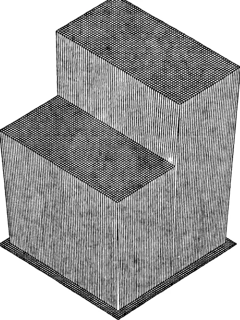
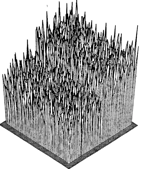
Figure 1 is a plot of a 64 x 64 image of 4096 real variables which represent a step

discontinuity of height 49.0. Figure 2 shows the same data degraded by additive Gaussian

noise with zero mean and standard deviation 24.5, half the step height. Linear approaches

to removing noise from Figure 2 invariably blur the step edge also. Nonlinear approaches

based on Equation 16 exhibit local optima and require qlobal optimization such as simulated

annealing, which is is slow. Figure 3 is the result of minimizing Equation 16 by using mean

field annealing of Equation 18. Clearly mean field annealing is able to recover the original

image from the degraded image. Figure 3 was obtained using an initial T

==

24 and a final T

=

.24 and a v

=

24.

Piecewise-linear restorations are similarly obtained by replacing the first difference in the

argument of the prior potential function V by the appropriate second difference [2] ·

6

Conclusions

The diffusion equation method of global optimization introduced by Kostrowicki and Piela

has been related to the more familiar method of global optrnization, simulated annealing.

nealing into a deterministic algorithm for optimizing real variables. Mean field annealing

prescribes a sequence of local minimizations at decreasing "temperatures" of a Gaussian

in-tegral of the original objective function. Except for terminology ("time" for "temperature"),

this is identical to Kostrowicki and Piela's method. Experimental results for large image

optimization problems were presented which support and extend Kostrowicki and Piela's

results.

7

Acknowledgements

We thank Stephen J. Garnier for writing the mean field annealing program and for producing

the figures.

References

[1]

G. L. Bilbro, T. K. Miller, W. E. Snyder and D. E. Van den Bout, M. W. White, and

R. C. Mann. Optimization by the Mean Field Approximation. In Advances in Neural

Network Information Processing Systems 1, pages 91-98. Morgan-Kauffman, San Mateo,

[2] Griff L. Bilbro and Wesley E. Snyder. Mean field annealing: An application to image

noise removal. Journal of Neural Network Computing, 1990.

[3]

Griff

L.

Bilbro, Wesley

E.

Snyder, Steven J. Garnier, and James

W.

Gault. Mean field

annealing: A formalism for constructing GNC-like algorithms. IEEE Transactions on

Neural Networks, 3(1), 1992. scheduled to appear.

[4]

Griff L. Bilbro, Wesley E. Snyder, and Reinhold C. Mann. The mean field minimizes relative entropy. Journal of the Optical Society of America A, 8(2):290-294, February

1991.

[5]

H.

P.

Hiriyannaiah, G.

L.

Bilbro, W.

E.

Snyder, and R. C. Mann. Restoration of

piecewise constant images via mean field annealing. Journal of the Optical Society

0/

America A, pages 1901-1912, December 1989.

[6]

S. Kirkpatrick, C. Gelatt, and

M.

Vecchio Optimization by simulated annealing. Science,

220(4598):671-680, May 1983.

[7]

J. Kostrowicki and

L.

Piela. Diffusion equation method of global minimization:

Perfor-mance for stnadard test functions. Journal of Optimization Theory and Applications,

69(2):269-284, May 1991.

[9] N. Metropolis, A. Rosenbluth, M. Rosenbluth, A. Teller, and E. Teller. Equations of

state calculations by fast computing machines. Chern. Physics, 21:1087-1092, 1953.

[10] W. E. Snyder, G. L. Bilbro, and D. E. Van den Bout. New techniques in

optimiza-tion. Technical Report NETR89-12, Center for Communications and Signal Processing,

NCSU, Raleigh, 27695, 1989.

[11] C. M. Soukoulis, K. Levin, and G. S. Grest. Irreversibility and metastability in