Simulation-Optimization Framework to Support Sustainable Watershed Development by Mimicking the Pre-development Flow Regime

(1)

ABSTRACT

PIERPONT, LAUREL HUGHES. Simulation-Optimization Framework to Support Sustainable Watershed Development by Mimicking the Pre-development Flow Regime. (Under the direction of Dr. E. Downey Brill).

The modification of land and water resources for human use alters the natural hydrologic flow regime of a downstream receiving body of water. The natural flow regime is essential for sustaining biotic structure and equilibrium within the ecosystem. A typical approach to achieve a hydrologically friendly development is to locate and design stormwater control structures, or Best Management Practices (BMPs), to match peak and minimum flows for design storms. A more aggressive strategy for environmentally sustainable development would ensure that there is no difference between pre- and post-development flow regimes for all storms and at all times through the design of development strategies that maintain the natural flow regime under post-development conditions at the watershed outlet. Many sub-catchments contribute to the composite flow at the watershed outlet of a large watershed, and at each of these sub-catchments, the flow regime may be altered, though the flow regime is maintained at the larger watershed level.

(2)

Simulation-Optimization Framework to Support Sustainable Watershed

Development by Mimicking the Pre-development Flow Regime.

by

Laurel Hughes Pierpont

A thesis submitted to the Graduate Faculty of North Carolina State University

In partial fulfillment of the Requirements for the degree of

Master of Science

Civil and Environmental Engineering

Raleigh, North Carolina 2008

Approved by:

_______________________________ ______________________________

Dr. E. Downey Brill, Jr., Dr. Emily Zechman

Committee Chair

(3)

ii

DEDICATION

“When one tugs at a single thing in nature, he finds it attached

to the rest of the world.”

- John Muir

This work is dedicated

to the love of my life;

to my family;

and to all the people who have inspired me along the way,

(4)

iii

BIOGRAPHY

Laurel Pierpont was born and raised in New England. She graduated from Brown University, in Providence, RI, with an honors Sc.B degree in Environmental Science. Her undergraduate thesis: Examination of Possible Hydrodynamic Controls on Bacteria Concentrations in the Runnins River, analyzed the relationships between streamflow and tidal dynamics with

(5)

iv

ACKNOWLEDGMENTS

I would like to acknowledge my committee members for all their encouragement and support over the past two years. I would like to personally thank Dr. Emily Zechman for her commitment and relentless desire to providing her students with the tools to perform their very best, and for teaching me what it truly means to work hard. I would like to thank Dr. Downey Brill for his energy and enthusiasm, for teaching me how to think critically, and for continuously challenging me. I would like to thank Dr. Margery Overton for her intellectually stimulating questions, and for all her guidance through the process of research. To all my committee members: thank you for believing in me and challenging me to perform my very best, I am truly grateful for all the knowledge, wisdom, and experience I have gained in my short time with you. I would also like to acknowledge Dr. Ranji Ranjithan for his technical guidance, support, and most of all friendship.

To my officemates and neighbors, thank you for always being there to lend a helping hand, and for asking important questions. Matt Clayton, Ted Ziegler, and Carrie Jackson: I don’t know if I could’ve survived this adventure without you. You have meant so much to me over the last two years and I know our friendships will continue to grow.

I would also like to thank my parents, who have provided me with so much support, guidance, and love over the years.

(6)

v

LIST OF FIGURES

Figure 1: RVA Target Establishment and the Frequency of Data Points that Fall within the

three Ranges. (Source Richter et. al 1998) ... 10

Figure 2: Counting IHA Mis-Hits using Monthly flows for October ... 12

Figure 3 : Design Procedure for Simulation-Optimization Method ... 15

Figure 4: Rouge River Watershed Geographic Reference (Source: Wayne County DOE/RPO)... 21

Figure 5: Gauged Streamflow Record for 50 years for the Middle Rouge River (Source: USGS) ... 21

Figure 6: Uniform Development Approach Solutions for Eight Gradients of Development . 25 Figure 7: Common Classification of Optimization Techniques ... 27

Figure 8: Optimization Development Approach Solutions for GA and NM Search Techniques at the 30% Development Constraint... 29

Figure 9: Examination of NM and GA Solutions at the 30% Development Constraint. ... 30

Figure 10: GA Solution Convergence for Trial 1 at 30% Modeled Development Level ... 31

Figure 11: GA Solution Convergence for Trial 2 at 30% Modeled Development Level ... 32

Figure 12: Non-Uniform Optimized IHA-SMHC versus Total Acreage Developed ... 33

Figure 13: Comparison of GA and NM search solutions for IHA-SMHC = 310... 36

Figure 14: GA 310 and GA 324 Development Distribution and Allocation Comparison... 38

Figure 15: Distribution of Development for Solutions at the 10% Modeled Development Level... 40

Figure 18: Distribution of Development for Solutions at the 25% Modeled Development Level. ... 41

Figure 21: Fraction of Total Possible Mis-Hits for 10% Development Level Solutions... 47

Figure 27: Fraction of Total possible Mis-Hits at each Modeled Development Level... 50

(8)

vii

LIST OF TABLES

Table 1 : Linkage Between Flow Parameters and Ecological Attributes (source Bragg et al

2005)...5

Table 2 : Biotic Group Response to a Flow Regulated Stream (source Bragg et al 2005). ...6

Table 3 : Indicators of Hydrologic Alteration Parameter Grouping and Identification. ...8

Table 4: Land Use Categories and Percentage of Total Drainage Area ... 19

Table 5: SWMM Parameter Inputs for Middle Rouge River Case Study... 23

Table 6: Total Developed Acreage and IHA-SMHC for Uniform Development Scenarios... 24

Table 7: Parameter Settings for GA Optimization Technique ... 28

Table 8: IHA-SMHC (for GA 30% solutions) versus the Absolute Total Change in Development between Solutions... 37

Table 9: Absolute Percentage Differences in Development Distributions for all Modeled Development Levels... 44

(9)

1

CHAPTER 1: Introduction

A goal of sustainable watershed development is to maintain and preserve the natural resources and processes that create and maintain an ecosystem’s diversity and integrity. Recent studies have shown a high degree of correlation between alterations in hydrologic flows and ecological and habitat attributes. As flows are easily and commonly measured and modeled, using hydrologic alterations as a basis for watershed management provides a promising direction to achieving sustainable development. Also, in many cases, pre-development flows have been measured and are available, thus enabling the definition of metrics that represent the departure from predevelopment conditions—a proper notion of sustainability.

(10)

2

CHAPTER 2: A Method for Mimicking the Predevelopment Flow Regime

2.1 Introduction

An appropriate metric for achieving sustainable development is embedded within the mechanistic link between the hydrologic flow regime and ecosystem health. Analysis of a long term record of pre-development flows would reveal a natural variability in the streamflow dataset. This natural tendency of fluctuation is a statistically significant aspect of the streamflow record. Variation of this flow regime due to watershed development, or other manipulations such as dams, can generate a shift or change in the natural variability of the streamflow. Success in mimicking the pre-development flow regime under post-development scenarios is therefore an essential step in achieving sustainable development and conserving ecosystem health.

(11)

3 parameters such as magnitude, rate, and frequency can concentrate in-stream pollutant loads, or simply offset ecosystem function due to varying hydrodynamics, leading to various degrees of ecological degradation (Carpenter et. al 1998, Baron et. al 2002, 2003, and Allan 2004). Studies have shown that the dynamics of ecosystem function and structure depend on this natural variability of the flow regime, thereby making it a good indicator of riverine health, (Poff and Allan 1995, Richter et al., 1997).

The methodology presented in this research to achieve sustainable development by mimicking the predevelopment flow regime involves many different components. The first main component is the discussion of relevant literature and background information on the definition of ecologically relevant metrics. From this review, the main methodology for establishing the hydrologic alteration evaluator metric is formed and presented. In addition, the hydrologic simulation of modeled futuristic scenarios of development, a key step in the methodology of mimicking the predevelopment flow regime, is also discussed.

2.2 Background Information

(12)

4 ecological quality on the basis of flow regime targets (Biggs et al 1990). Development of these flow regime parameters involved several studies including Clausen and Biggs (1997;1998); who identified hydrologic indices with relevance to invertebrate ecology, Mader et al (1997), who also developed ecology-related classifications for flow parameters, and Puckridge et al (1998), who devised 23 hydrological measures based on aspects of flow variability in relation to fish biology.

(13)

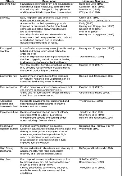
5 Table 1 : Linkage Between Flow Parameters and Ecological Attributes (source Bragg et al 2005).

Effects Description Literature Sources

Declining flow Ranunculus cover positively, and abundance of Ruse and Love (1997) filamentous algae negatively, correlated with Kobayashi et al. (1998) flow velocity. Also changes in phytoplankton Vieira et al. (1998) and the associated zooplankton communities. Wilby et al. (1998) Low flow Early migration and shortened travel times Quinn et al. (1997)

observed for salmonid fish. Wallace and Collins (1997) Access of fish to their spawning grounds Duffy (1996)

impeded or prevented. On the other hand, Hendry and Cragg-Hine (1996) some species select spawning sites with Keckeis et al. (1997)

low current velocity. Moir et al. (1998)

Mortality of salmon due to elevated water Hendry and Cragg-Hine (1996) temperature and deoxygenation; also reduced

reproductive success due to stranding, dewatering and freezing of redds.

Prolonged Loss of salmon spawning areas, juvenile rearing Hendry and Cragg-Hine (1996) low flow habitat and ‘living room’. Adult fish fail to

enter the river

Influx of sulphate-rich saline groundwater to Donnelly et al. (1997) the river, triggering a chain of events leading

to development of a cyanobacterial bloom.

Very low constant flow (below natural low flow) Gustard et al. (1987) may severely reduce wetted area and hence

the overall productivity of the river.

Low winter flow Macrophyte mortality due to frost exposure Rorslett and Johansen (1996) (in Norway, nuisance lotic vegetation can be

controlled by draining rivers in winter).

Flow cessation Positive selection for invertebrate species that Gustard et al. (1987) can survive in pools and under rocks.

Silting and fen formation on floodplain that is Girel and Manneville (1998) cut off from the main channel.

Alternating Reversible development of submerged and Theilling et al. (1996) decline and floating-leaved aquatic plants in channel

increase in flow borders and backwaters.

Increase in flow Decline of macrophytes as current velocity Brierley et al. (1989) rises from 0.01 to 0.1ms 1, and loss Chambers et al. (1991) of submerged species by scouring under Rorslett and Johansen (1996) abnormally high flow conditions.

Flooding of Increase in phytoplankton production. Robinson et al. (1997a; 1997b) Riparian Buffers Decline in abundance of nonplanktonic algae and Woltemade (1997)

density of emergent macrophytes. Loss of aquatic vegetation due to persistent high water, sedimentation, and associated resuspension of sediments which in turn impedes light penetration.

High Spring Severe reduction in abundance and diversity of DeBrey and Lockwood (1990) Discharge aquatic insects, with rapid subsequent

recovery of all groups except Diptera.

High flow Fish respond to even small increases in flow Schaffter (1997) by moving upstream, but access to the river Bergeron et al. (1998) mouth is limited at high flows.

Drifting goby larvae survive long enough to Moriyama et al. (1998) reach the sea only in above-normal flow

(14)

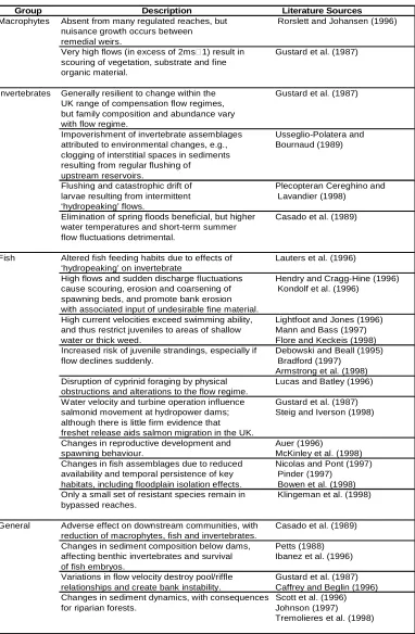
6 Table 2 : Biotic Group Response to a Flow Regulated Stream (source Bragg et al 2005).

Group Description Literature Sources

Macrophytes Absent from many regulated reaches, but Rorslett and Johansen (1996) nuisance growth occurs between

remedial weirs.

Very high flows (in excess of 2ms 1) result in Gustard et al. (1987) scouring of vegetation, substrate and fine

organic material.

Invertebrates Generally resilient to change within the Gustard et al. (1987) UK range of compensation flow regimes,

but family composition and abundance vary with flow regime.

Impoverishment of invertebrate assemblages Usseglio-Polatera and attributed to environmental changes, e.g., Bournaud (1989) clogging of interstitial spaces in sediments

resulting from regular flushing of upstream reservoirs.

Flushing and catastrophic drift of Plecopteran Cereghino and larvae resulting from intermittent Lavandier (1998)

‘hydropeaking’ flows.

Elimination of spring floods beneficial, but higher Casado et al. (1989) water temperatures and short-term summer

flow fluctuations detrimental.

Fish Altered fish feeding habits due to effects of Lauters et al. (1996) ‘hydropeaking’ on invertebrate

High flows and sudden discharge fluctuations Hendry and Cragg-Hine (1996) cause scouring, erosion and coarsening of Kondolf et al. (1996)

spawning beds, and promote bank erosion with associated input of undesirable fine material.

High current velocities exceed swimming ability, Lightfoot and Jones (1996) and thus restrict juveniles to areas of shallow Mann and Bass (1997) water or thick weed. Flore and Keckeis (1998) Increased risk of juvenile strandings, especially if Debowski and Beall (1995) flow declines suddenly. Bradford (1997)

Armstrong et al. (1998) Disruption of cyprinid foraging by physical Lucas and Batley (1996) obstructions and alterations to the flow regime.

Water velocity and turbine operation influence Gustard et al. (1987) salmonid movement at hydropower dams; Steig and Iverson (1998) although there is little firm evidence that

freshet release aids salmon migration in the UK.

Changes in reproductive development and Auer (1996)

spawning behaviour. McKinley et al. (1998) Changes in fish assemblages due to reduced Nicolas and Pont (1997) availability and temporal persistence of key Pinder (1997)

habitats, including floodplain isolation effects. Bowen et al. (1998) Only a small set of resistant species remain in Klingeman et al. (1998) bypassed reaches.

General Adverse effect on downstream communities, with Casado et al. (1989) reduction of macrophytes, fish and invertebrates.

Changes in sediment composition below dams, Petts (1988) affecting benthic invertebrates and survival Ibanez et al. (1996) of fish embryos.

Variations in flow velocity destroy pool/riffle Gustard et al. (1987) relationships and create bank instability. Caffrey and Beglin (1996) Changes in sediment dynamics, with consequences Scott et al. (1996)

for riparian forests. Johnson (1997)

(15)

7

2.3 Ecologically Relevant Metrics

(16)

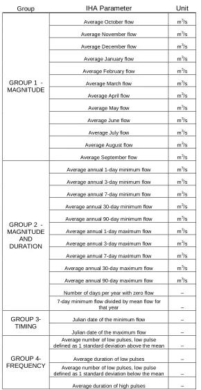
8 Table 3 : Indicators of Hydrologic Alteration Parameter Grouping and Identification.

Group IHA Parameter Unit

Average October flow m3/s

Average November flow m3_/s

Average December flow m3/s

Average January flow m3/s

Average February flow m3_/s

Average March flow m3/s

Average April flow m3/s

Average May flow m3/s

Average June flow m3/s

Average July flow m3/s

Average August flow m3/s

GROUP 1 - MAGNITUDE

Average September flow m3_/s

Average annual 1-day minimum flow m3/s

Average annual 7-day minimum flow m3_/s

Average annual 1-day maximum flow m3/s

Number of days per year with zero flow –

GROUP 2 - MAGNITUDE

AND DURATION

7-day minimum flow divided by mean flow for

that year –

Julian date of the minimum flow –

GROUP 3- TIMING

Julian date of the maximum flow – Average number of low pulses, low pulse

defined as 1 standard deviation above the mean –

Average duration of low pulses – Average number of low pulses, low pulse

defined as 1 standard deviation below the mean –

GROUP 4- FREQUENCY

(17)

9 Table 3 (continued).

Rise rate−mean of all positive differences m3/s/day

Fall rate−mean of all negative differences m3_/s/day

GROUP 5- RATE OF CHANGE

Number of flow reversals –

(18)

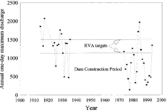
10

2.4 Application of Indicators of Hydrologic Alteration (IHA) Methodology

The IHA methodology was originally designed with intent to help scientists and policymakers examine changes in flow regimes caused by dams. As researchers are discovering, however, it can be applied to a large range of hydrologic and ecological studies. The hydrologic alteration is quantified by analyzing the medians and measures of variability between the predevelopment period and the post-development period using the Range of Variability Approach (RVA) (Richter et al, 1997). This method allows for the calculation of a percentage of change in the ecologically relevant streamflow statistics. The RVA is used to help prescribe restoration targets (Figure 1). The ecosystem flow restoration targets are numerical ranges within which the streamflow statistical variability should be maintained.

Figure 1: RVA Target Establishment and the Frequency of Data Points that Fall within the three Ranges. (Source Richter et. al 1998)

(19)

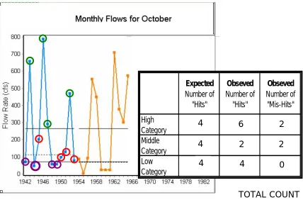
11 calculate change in variability based on the IHA is to count the median flow data points within three target ranges: low, medium, and high. When both the pre- and post-development datasets maintain the same frequency (number of data points) within the low, medium, and high range, the goal has been achieved. When the data points do not fall within the same range, it is considered an IHA “Mis-Hit.” Each of the 33 IHA parameters will have an associated Mis-Hit, ranging from zero to some maximum count which is dependent on the number of years modeled in the scenario. By summing these Mis-Hits over the 33 IHA indices the total count reflects a degree of ecological degradation. In this methodology, the sum of Mis-Hits is used as a metric for hydrologic alteration. Figure 2 shows an example of this process for obtaining the Mis-Hit count for the Monthly Flows for October parameter over a total of 12 predevelopment years (1941-1952) and 12 post-development years (1954-1965). The expected number of Hits refers to the pre-development record, where the observed number of Hits refers to the post-development record, and the discrepancy between

(20)

12 Figure 2: Counting IHA Mis-Hits using Monthly flows for October

2.5 Stormwater Management Model (SWMM)

Watershed hydrologic models are important tools for addressing the increasing demands and problems related to water resources management and implementation. Models are used to estimate and evaluate the quantity and quality constituents of streamflow and urban runoff, impacts of reservoir operations, urban land development, and a range of other processes (Wurbs, 1998). The significance of using such a mathematical model is the ability to isolate the effects of specific aspects of urban development by holding all other watershed

Expected

Number of "Hits"

Obseved

Number of "Hits"

Obseved

Number of "Mis-Hits"

High

Category 4 7 3

Middle

Category 4 3 1

Low

Category 4 2 2

6

2

4

2

0 4

4

(21)

13 properties constant. This enables engineered decisions to be made efficiently, ensuring future watershed sustainability. One of the main components of this research's methodology employs EPA's Storm Water Management Model (SWMM) to simulate urban runoff of futuristic development scenarios (Huber et al., 1992).

SWMM was developed between 1969 and 1971, and was one of the first models to simulate urban runoff from both a quantity and quality standpoint. Written in Fortran, the model is composed of a series of algorithms for the various operating blocks. SWMM is essentially a surface water budget model, and the first of its kind able to represent urban runoff and combined sewer overflow issues with associated cost estimates for storage and/or treatment controls. SWMM has the capability to combine hydrographs at different locations into a single hydrograph time series, representing just one location: the watershed outflow point. Among the many complexities of SWMM, the major components are the precipitation, infiltration, and urban runoff techniques.

(22)

14

2.6 Final Remarks

(23)

15

CHAPTER 3: Simulation-Optimization Framework to Support

Sustainable Watershed Development

3.1 Introduction

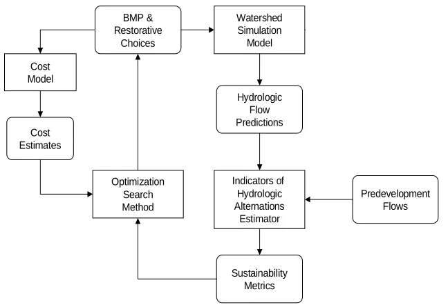
Human manipulation of water flows due to development has been a leading cause of ecological degradation. Using the IHA/RVA method to assess the hydrologic alteration associated with each long-term development pattern, a plan for watershed development can be identified to specify the spatial location and total of quantity of allowable imperviousness that will minimize the IHA parameter alteration. An overview of the design procedure to address this watershed management problem is outlined in Figure 3.

Figure 3 : Design Procedure for Simulation-Optimization Method

BMP & Restorative

Choices

Hydrologic Flow Predictions Watershed Simulation Model

Predevelopment Flows Indicators of

Hydrologic Alternations Estimator Optimization

Search Method

Water Quality Predictions

Sustainability Metrics Cost

(24)

16 As Figure 3 outlines, this approach to sustainable development involves many different complex relationships between optimization, cost, watershed simulation, and hydrologic flow predictions.

3.2 Mathematical Model Formulation

The mechanism employed to address the causative link between increasing levels of imperviousness and ecosystem preservation is a mathematical optimization model. As outlined in Figure 3, BMP and restorative choices are iteratively updated and modified depending upon the IHA-SMHC results. However, design choices could also be user modified depending on the cost analysis.

The underlying goal of the optimization-simulation methodology is to find the optimal development pattern that has the least potential impact in altering the hydrologic flow regime.

The mathematical model for this problem is as follows;

(3.1)

and

(3.2)

The penalty function is incorporated to aid the performance evaluation of the objective function and discount solutions that do not satisfy the one sided minimum development constraint. This can be represented as;

to subject

∑ ∑

= =

=IHA P j

C

i i j

M Alteration

Minimize

_ 1 1

T A P _n

SC n

n ≥

∑

=1

n n U

(25)

17 (3.3)

and (3.4)

(3.5)

Where Mij= number of Mis-Hits in each category i for each IHA Parameter j; C =

number of categories for each IHA parameter (3 – High, Mid, Low); IHA_P = number of IHA parameters (33); Pn = percent imperviousness in subcatchment n; An = acreage of

subcatchment n; SC = number of subcatchments in the watershed; T = total developed acreage in the watershed; and Un = upper bound on the amount of development allowed in

each subcatchment n. Specification of the upper bound deals with the assumption that for a given subcatchment 100% development is generally not attainable due to common construction practices and aesthetic nature of architectural design which almost always includes greenery around the perimeter of buildings, houses, and other structures.

The solution to this problem will identify the development pattern that minimizes the total hydrologic alteration (Eq (3.3)), subject to total level of development constraints (Eqs (3.4) and (3.5)). The expressions presented here can be modified and evaluated based on the user's specific model and criteria; however, the following subsections will employ these functions for the analysis of a specific case study.

Penalty function to enforce development constraint;

Violation K M f Minimize P IHA j C i i

j + ×

=

∑ ∑

= = _ 1 1 n n U

P < ∀ n

(26)

18

3.3 Illustrative Application to a Watershed Development Pattern

3.3.1 Background Information

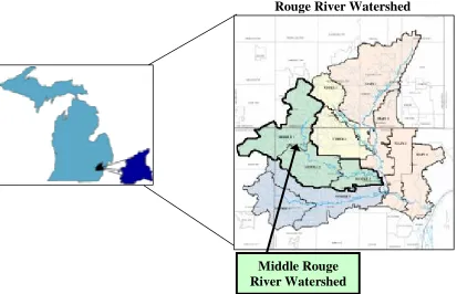
The Rouge River Watershed encompasses approximately 438 square miles in southeastern Michigan and contains 1.5 million residents. The watershed covers three counties; Wayne, Oakland, and Washtenaw, and contains 127 river miles. Figure 4 shows the Rouge River and its four major branches; Lower, Middle, Upper, and Main. This figure also shows the boundaries of the 11 major subwatersheds, which include the Upper 1, Upper2, Lower 1, Lower 2, Middle 1, Middle 2, Middle 3, Main 1, Main 2, Main 3, and Main 4. The Rouge River watershed outlet discharges into the Detroit River, which eventually drains into Lake Erie. The Rouge River watershed is 50% urbanized with less than 25% undeveloped land. For modeling purposes ten different land uses categorize the Rouge River watershed and are listed in detail in Table 4.

(27)

19 Table 4: Land Use Categories and Percentage of Total Drainage Area

The current Rouge River modeling effort can be described in three phases. The first phase consists of several small area models used to simulate flows, pollutant loads and concentration from specific wetlands, ponds, or other localized areas. The second modeling phase involves a sewer system model in addition to a pollutant loading model. Both of these models simulate pollutant generation by subarea and cover the entire watershed. The third phase simulates instream flows for the four main subwatersheds and uses pollutant loading inputs from phase two to characterize instream water quality.

(28)

20 determine overall pollutant loading reduction for sustainability and management purposes. In addition EPA’s SWMM model is used to model the hydrology of all natural drainage areas with storm sewers. A SWMM RUNOFF/TRANSPORT model was developed in 1994 and is used to model all the CSOs entering the river. By utilizing USGS streamflow gauges for continuous data, as well as inflow hydrographs from the CSO and RUNOFF models combine to then generate a one-dimensional river model referred to as the SWMM TRANSPORT model.

The Middle Rouge River, 70,000-acres in size, is one of the four main subwatersheds contributing to the Rouge River (Figure 4). Water quality improvements have been an ongoing effort of policymakers in the Detroit and suburban areas. Overflowing CSO’s and highly polluted storm water runoff has left city planners scrambling for answers. EPA has been funding the Rouge River Wet Weather Demonstration program since the early eighties. In addition, multiple TMDL programs are underway.

(29)

21 Figure 4: Rouge River Watershed Geographic Reference (Source: Wayne County DOE/RPO)

Figure 5: Gauged Streamflow Record for 50 years for the Middle Rouge River (Source: USGS) Middle Rouge

River Watershed

(30)

22 There is a subtle transformation of the daily streamflow averages, streamflow variability, and median streamflow values from the 1960’s to the 1990’s, highlighting potential human-induced impact. The Baseline Data Summary report of 2000 also highlights water quality transitions in what might be considered as the post-development period. Rapid changes in dissolved oxygen and nutrients are reported, in addition to reported increases in eutrophication and aesthetic degradation (Baseline Data Summary, 2000).

3.3.2 Model Parameters

The Middle Rouge River watershed is modeled using SWMM, which for the particular area was developed and calibrated by local environmental consultants in 1994 (Camp Dresser & McKee, Inc., 1994). At the time of model development, the seven subcatchments had an average of 5.8% imperviousness. Due to the minimal, if any, amount of ecological and biological samples collected during these conditions, efforts to transition the Middle Rouge River to some unknown predevelopment flow regime is impossible. The Middle Rouge River is, however, the least developed out of the four main subwatersheds mentioned earlier, and thus a perfect candidate for resembling predevelopment conditions in this analysis.

(31)

23 areas reflect the extent of the acreage modeled in this research. The slope refers to the ground slope of each subcatchment, and the initial imperviousness reflects the pre-development modeled conditions.

Table 5: SWMM Parameter Inputs for Middle Rouge River Case Study

3.3.3 Uniform Development Approach

The uniform development approach simulates urban runoff in the watershed without a mathematical optimization component for iterative development pattern decision making. Uniform development essentially reflects an unsustainable approach to watershed development because it sequentially increases the imperviousness in each subcatchment without considering the associated changes to the natural flow regime taking place. Sensitive areas in the watershed that become developed go unmitigated in this approach. The IHA/RVA technique described previously is used to model twenty-years of daily average streamflow values for a total of eight different uniform development scenarios. Each uniform post-development scenario is evaluated against the pre-development flow regime to obtain a corresponding IHA-SMHC for that record. The pre-development condition is represented with an IHA-SMHC equal to zero, and acts as the baseline. The uniform post-development

Subcatchment ID Total Area _(acres) Slope (%)

Imperviousness (%)

1 757.12 0.00818 4.619

2 739.66 0.01064 5.884

3 1851.28 0.00972 5.444

4 2489.12 0.00714 9.733

5 2057.75 0.00636 3.849

6 2372.07 0.00414 4.509

(32)

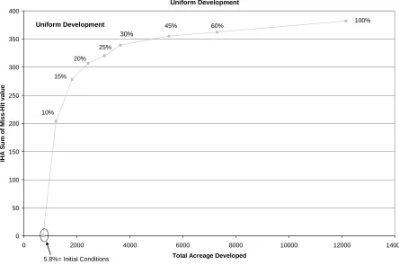
24 scenarios include 10, 15, 20, 25, 30, 45, 60, and 100% imperviousness. Figure 6 shows the resulting IHA-SMHC versus total developed acreage for these eight scenarios, and the results are summarized in Table 6.

As the literature has revealed, the link between development induced manipulation of the flow regime and biotic change is strong, and therefore we are assuming that a higher IHA-SMHC correlates with increased ecosystem degradation. As Figure 6 highlights, the increase in IHA-SMHC is extremely responsive in the 6% to 45% post-development range showing an increase in Mis-Hits from zero to 355. Further increase from the 45% IHA-SMHC level to 100% only yields 27 additional Mis-Hits, a seemingly small IHA-IHA-SMHC increase for 55% additional imperviousness. This guides a notion that once a certain level of development has been reached without proper watershed management techniques, ecosystem damage has occurred, and development to 100% induces no further significant increase in the IHA-SMHC.

Table 6: Total Developed Acreage and IHA-SMHC for Uniform Development Scenarios

DEVELOPED ACREAGE IN EACH SUBCATCHMENT

Subcatchment ID

Uniform 5.8%

Uniform 10%

Uniform 15%

Uniform 20%

Uniform 25%

Uniform 30%

Uniform 45%

Uniform 60%

Uniform 100%

1 35 76 114 151 189 227 341 454 757

2 44 74 111 148 185 222 333 444 740

3 101 185 278 370 463 555 833 1111 1851

4 242 249 373 498 622 747 1120 1493 2489

5 79 206 309 412 514 617 926 1235 2058

6 107 237 356 474 593 712 1067 1423 2372

7 125 189 284 378 473 568 851 1135 1892

Total area 733 1216 1824 2432 3040 3648 5472 7295 12159

(33)

25

Comparing IHA-SMHC with Total Developed Acreage for Uniform Development

0 50 100 150 200 250 300 350 400

0 2000 4000 6000 8000 10000 12000 14000

Total Acreage Developed

IH

A

S

u

m

o

f

M

is

s

-H

it

v

a

lu

e

5.8%= Initial Conditions 30%

45% 60% 100%

Uniform Development

10% 15%

20% 25%

Figure 6: Uniform Development Approach Solutions for Eight Gradients of Development

3.3.4 Optimized Development Approach

(34)

26 3.3.4.1 Nelder Mead and Genetic Algorithm Search Techniques

(35)

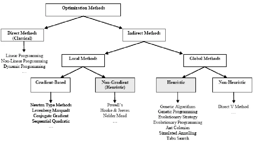
27 Figure 7: Common Classification of Optimization Techniques

3.3.4.2 Hybrid Algorithm Search Technique

(36)

28

3.3.5 Results and Discussion

To explore the search methods, one level of development is selected, and ten random trials are executed for the NM and GA approaches as separate searches, with parameter settings outlined in Table 7, at the post-development level of 30%. These parameters are set at typical values, and could be explored in future analyses.

Table 7: Parameter Settings for GA Optimization Technique

Parameter Value

Population Size 50

Probability of crossover (average % of strings that undergo crossover) 60% Uniform crossover rate (average % of decision variables crossed over in a string) 28%

Mutation uniform

Generation number at which the search stops, Gmax 100

(37)

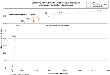
29 Figure 8: Optimization Development Approach Solutions for GA and NM Search Techniques at the 30% Development Constraint

Comparing IHA-SMHC with Total Developed Acreage for Uniform and Non-Uniform Development

0 50 100 150 200 250 300 350 400

0 2000 4000 6000 8000 10000 12000 14000

IH

A

S

u

m

o

f

M

is

s

-H

it

C

o

u

n

t

UD

Genetic Algorithm Nelder Mead

5.8%= Initial Conditions

30% 45%

60%

100%

Uniform Development

10% 15%

20% 25%

(38)

30 Comparing IHA-SMHC with Total Developed Acreage for

Uniform and Non-Uniform Development

300 310 320 330 340 350 360

3500 4000 4500 5000 5500 6000

IH

A

S

u

m

o

f

M

is

s

-H

it

C

o

u

n

t

UD

Genetic Algorithm Nelder Mead

30%

45%

Figure 9: Examination of NM and GA Solutions at the 30% Development Constraint.

(39)

31 approach is therefore the sequential combination of the GA to NM after the GA has completed 15 generations. The NM begins its local search with this seeded solution from the GA. From a computing time efficiency standpoint this hybrid approach is far superior. Further examination of when to stop the GA is warranted to potentially further reduce the computing time. This analysis would involve examination of the total population of solutions at each generation of the GA beginning with generation one. This further exploration will be addressed later in Section 5: Modeling to Generate Alternatives.

Figure 10: GA Solution Convergence for Trial 1 at 30% Modeled Development Level

GA Solution TRIAL 1 at the 30% Modeled Development Level

290 300 310 320 330 340 350 360

2 4 6 8 10 12 14 16 18 20 22 24 26 28 30 32 34 36 38 40 42 44 46 48 50 52

Generation Count

O

b

je

c

ti

v

e

V

a

lu

e

(40)

32 Figure 11: GA Solution Convergence for Trial 2 at 30% Modeled Development Level

The hybrid approach was applied to the entire development curve ranging from 10% (1,216 acres developed) to 45% (5,472 acres developed). This procedure was based on the results at the 30% post-development level using the two individual search techniques. For each of the six development levels explored, five random trials were executed and are presented in Figure 12. The optimized solutions are associated with less hydrologic alteration than the uniform development. One of the many benefits of the simulation-optimization framework is that it allows policymakers to allocate land for development with knowledge of the predicted hydrologic alterations associated with that scenario. Based on the watershed’s ecosystem flow regime target (something that could change depending upon the site-specific initiatives), land development can be planned accordingly as to not exceed some predefined threshold. If the threshold is set at 300 IHA-SMHC, for example, uniform

GA Solution TRIAL 2 at the 30% Modeled Development Level

290 300 310 320 330 340 350 360

2 4 6 8 10 12 14 16 18 20 22 24 26 28 30 32 34 36 38 40 42 44 46 48 50

Generation Count

O

b

je

c

ti

v

e

F

u

n

c

ti

o

n

V

a

lu

e

(41)

33 development would allow ~18% imperviousness, whereas the optimized scheme would allow nearly 30% imperviousness according to Figure 12. This increase in the amount of developable land made possible by the optimization method is a meaningful change and increased benefit from the standpoint of the watershed managers.

Comparing IHA-SMHC with Total Developed Acreage for Uniform and Non-Uniform Development

0 50 100 150 200 250 300 350 400

0 2000 4000 6000 8000 10000 12000 14000

IH

A

S

u

m

o

f

M

is

-H

it

C

o

u

n

t

UD Hybrid

5.8%= Initial Conditions

30% 45%

60%

100% Uniform Development

10% 15%

20% 25%

Non-Uniform Development

(42)

34

3.4 Final Remarks

(43)

35

CHAPTER 4: Comparative Analysis of Development Solutions

4.1 Introduction

When two solutions with the same resulting hydrologic alteration have very different spatial distributions of development, the decision for which development plan to proceed with may seem a daunting task. Therefore, comparative analysis of development solutions is an important step in the overall procedure of this methodology, and takes into account the main driving forces embedded in this approach, while also acknowledging unmodeled issues. Firstly, the role of the subcatchments in the development allocation tradeoff can help to differentiate between solutions. Secondly, the IHA-SMHC metric and its corresponding 33 parameters change as a function of development, and the valuable information they provide as they change can help guide policymakers to differentiate solutions. Unmodeled issues include watershed site-specifics, namely distinct topographical regions, or ecologically critical sections that must be set aside as non-developable. In addition, the ability to implement flexible development allocation from a political and legal standpoint may change current development strategies.

4.2 Watershed Development Allocation Tradeoff

(44)

36 acreage between the two solutions is 1,577 acres, a large amount considering the 30% uniform development acreage is 3,648 acres. This result suggests a non-unique mapping from decision space to objective space, specifically; different development patterns in the watershed can produce the same resultant hydrologic alteration. As Figure 13 shows, two solutions (310GA and 310NM) have distinct development distributions among the seven subcatchments, yet maintain the same hydrologic alteration (IHA-SMHC) of 310. Subcatchments two and six have the most similar development, with subcatchment seven yielding the largest difference between solutions at nearly 620 acres (Figure 13). From the standpoint of the IHA-SMHC, there is no difference between the two solutions. The choice between the two solutions must now be left to policymakers to simultaneously consider unmodeled issues.

Figure 13: Comparison of GA and NM search solutions for IHA-SMHC = 310 Non-Uniform Optimized Development Pattern for 30%

0 200 400 600 800 1000 1200 1400

1 2 3 4 5 6 7

Subcatchment ID

D

e

v

e

lo

p

e

d

A

c

re

a

g

e

(

a

c

re

s

)

(45)

37 Further analysis of the ten executed solutions and their corresponding difference in development was performed for the GA solutions whose total development amongst solutions remained more consistent than that of the NM solutions. Table 8 outlines the absolute differences in development for the ten GA solutions modeled at the 30% development level. This difference can be mathematically defined as:

∑

=

−

7

1

n

nj nj i n

niA P A

P for all pairs of solutions (i,j) (4.1)

Where P_n= percent developed land in subcatchment n, and An = acreage of subcatchment n.

Table 8: IHA-SMHC (for GA 30% solutions) versus the Absolute Total Change in Development between Solutions.

The smallest and largest differences in development are highlighted grey in Table 8 with values of 271 and 4,555 acres, respectively. The smallest difference in land development distribution corresponds to solutions 313 and 314, an IHA-SMHC difference of just one. The largest change in the distribution of development is found between solutions 312 and 316. The difference in the development distribution between these two solutions is

310 312 313 314 316 319 321 323 324 309

310 - 3169 2361 2491 1791 2193 1044 2501 1566 2455

312 - 2934 2854 4555 1562 3372 2261 1976 1396

313 - 271 2495 2753 1837 2954 3086 2551

314 - 2335 2704 2001 2882 3037 2527

316 - 3325 2004 2626 2886 3648

319 - 2224 832 1263 1821

321 - 2056 1611 2401

323 - 1696 2431

(46)

38 4,555 acres, and yet the difference in IHA-SMHC is four. One of the largest discrepancies in IHA-SMHC for the ten solutions evaluated is 14, and corresponds to solutions 324 and 310. The difference in development between these two solutions is 2,455 acres (Figure 14). In this example, although the development patterns appear similar, the IHA-SMHC alludes to a large discrepancy between them. Not only do these results show the complex tradeoff between IHA-SMHC and total development, but also the variety of feasible development pattern allocation plans for seemingly similar and different IHA-SMHC objectives.

Figure 14: GA 310 and GA 324 Development Distribution and Allocation Comparison

Because of the increased computational efficiency with the hybrid approach, examination of six different development levels was performed. The six development levels are: 10, 15, 20, 25, 30, and 45%. The distribution of development within the watershed

Non-Uniform Optimized Development Pattern for 30%

0 200 400 600 800 1000 1200 1400

1 2 3 4 5 6 7

Subcatchment ID

D

e

v

e

lo

p

e

d

A

c

re

a

g

e

(

a

c

re

s

)

(47)

39 amongst the seven subcatchments proved to be unique even for solutions with the same IHA-SMHC. For the six development levels evaluated, only 45% had all five solutions with the same IHA-SMHC. At other development levels, all five executed solutions had both unique development allocations and IHA-SMHC values. Analysis and comparison of these results is included in Figures 15 through 20.

At the 10% level, the development allocation is somewhat uniformly spread with the exception of subcatchment four which accounts for the largest percent of total development. At 15% development, subcatchment seven accounts for the majority of development. The 20% level shows subcatchments five and seven reflecting nearly 50% of the total development. At the 25% level, subcatchments five and seven again reflect the largest portion of development. In the 30% and 45% solutions, there is a more uniform distribution of the majority of development among subcatchments three, four, and five, with subcatchment six accounting for the smallest percentage of total development.

(48)

40 Figure 15: Distribution of Development for Solutions at the 10% Modeled Development Level

Figure 16: Distribution of Development for Solutions at the 15% Modeled Development Level

Percent of Total Development Represented in each Subcatchment for five Simulation-Optimization Solutions

0 10 20 30 40 50 60

1 2 3 4 5 6 7

Sub Catchment ID

P e rc e n t o f T o ta l D e v e lo p m e n t (% )

Solution 1 Solution 2 Solution 3 Solution 4 Solution 5

0 10 20 30 40 50 60

1 2 3 4 5 6 7

(49)

41 Figure 17: Distribution of Development for Solutions at the 20% Modeled Development Level

Figure 18: Distribution of Development for Solutions at the 25% Modeled Development Level.

0 10 20 30 40 50 60

1 2 3 4 5 6 7

0 10 20 30 40 50 60

1 2 3 4 5 6 7

(50)

42 Figure 19: Distribution of Development for Solutions at the 30% Modeled Development Level.

Figure 20: Distribution of Development for Solutions at the 45% Modeled Development Level.

0 10 20 30 40 50 60

1 2 3 4 5 6 7

0 10 20 30 40 50 60

1 2 3 4 5 6 7

(51)

43 In each of the modeled development levels the distribution of imperviousness in subcatchment six remains consistently one of the smallest. For the 45% development level subcatchments one and two account for less of the total development than subcatchment six. This high degree of variability in the distribution of development among the five executed solutions alludes to a fairly flexible allocation of development at all modeled percentages. To grasp the range of this flexibility, examination of just how different these solutions are needs to be analyzed. One way to represent this difference is to compare the percentage of total development differences across all seven subcatchments for any given two solutions. Mathematically, this can be represented as:

for all pairs of solutions (i,j) (4.2)

where:

∑

=

= ₇

1

n

ni ni

ni ni ni

A P

R

Rni refers to the percent of total development that is reflected in subcatchment n for solution i,

ni

P refers to the percent developed land in subcatchment n for solution i, and Ani refers to the

acreage of subcatchment n for solution i.

Table 9 outlines the absolute differences between the executed solutions for all modeled development levels. This highlights how different the development distributions are from one solution to another normalizing for the difference in total acreage developed. The 10% level shows the smallest minimal difference amongst its solutions at 0%, meaning that

∑

=

−

7

1

n

nj i

n

R

(52)

44 at least two of the five executed solutions are identical for development in all seven subcatchments. The 30% level exhibits the highest maximal difference between solutions at 105%. Because this analysis is an absolute difference, the positive and negative differences between any two solutions are counted positively and therefore can result in a greater than 100% difference. The largest average difference for all five executed solutions occurs at the 20% modeled development level with a value of 75.1%. This suggests that the flexibility in development allocation is greatest at this modeled percentage level. Conversely, the 10% and 45% show the smallest average differences between solutions, and suggest that minimal amount of development alternatives exist at these levels.

Table 9: Absolute Percentage Differences in Development Distributions for all Modeled Development Levels

In summary, this comparative analysis shows that the maximal flexibility in development alternatives exists in the elbow of the tradeoff curve around the 20% modeled development level. Less flexibility in development alternatives occurs at opposite ends of the elbow: the 10% and 45%. A difference in the IHA-SMHC for any two solutions can

Modeled Development

Level

Max Difference

Min Difference

Average Difference

10% 71% 0% 28.4%

15% 67% 27% 47.2%

20% 103% 21% 75.1%

25% 84% 30% 54.8%

30% 105% 7% 69%

(53)

45 sometimes refer to a large difference in their development distributions, but as noted at the 45% development level this is not always the case.

4.3 Hydrologic Alteration Metrics

As previously introduced, the purpose of the 33 IHA flow metrics is to characterize statistical properties of the flow regime over a long-term horizon. Each metric has been proven to be associated with some influence on the ecosystem. The evaluator metric, IHA-SMHC, has been shown to increase with uniform development levels (Figure 6), but improve under optimized conditions (Figure 12). As Figure 6 also shows, the increase in IHA-SMHC is not linear with respect to the increase in development. If we consider each of the five solutions executed at the six modeled development levels, the overall change exhibited by the Mis-Hit counts is an important characteristic of each of the solutions. Results for the fraction of possible Mis-Hits fulfilled by each solution are summarized in Table 10. Figures 21 through 26 show the fraction of possible Mis-Hits within each IHA-Group for all solutions at the 10, 15, 20, 25, 30, and 45% development levels, respectively.

(54)

46 Table 10: Fraction of Possible Mis-Hits for each Executed Solution at all Modeled Development Levels

Categorized by IHA-Group

10%

15%

20%

25%

30%

45%

Solution IHA-SMHC Group 1 Group 2 Group 3 Group 4 Group 5

Seed 1 1 0.00 0.00 3.57 0.00 0.00

Seed 2 2 0.60 0.00 3.57 0.00 0.00

Seed 3 2 0.60 0.00 3.57 0.00 0.00

Seed 4 1 0.00 0.00 3.57 0.00 0.00

Seed 5 164 33.93 35.71 7.14 37.50 57.14

Seed 1 227 44.05 57.74 10.71 37.50 76.19

Seed 2 216 44.05 52.98 10.71 33.93 73.81

Seed 3 216 43.45 52.98 10.71 33.93 76.19

Seed 4 215 42.26 52.98 10.71 35.71 76.19

Seed 5 211 42.86 51.19 10.71 35.71 71.43

Seed 1 268 56.55 65.48 17.86 37.50 88.10

Seed 2 271 57.14 64.88 25.00 41.07 85.71

Seed 3 269 57.14 65.48 17.86 37.50 88.10

Seed 4 261 55.95 63.10 14.29 35.71 88.10

Seed 5 269 57.14 65.48 14.29 37.50 90.48

Seed 1 293 62.50 72.62 21.43 41.07 88.10

Seed 2 294 63.69 71.43 21.43 42.86 88.10

Seed 3 298 64.88 71.43 25.00 44.64 88.10

Seed 4 298 63.10 73.21 21.43 46.43 88.10

Seed 5 288 61.90 69.64 21.43 42.86 88.10

Seed 1 307 68.45 72.62 21.43 48.21 88.10

Seed 2 306 66.67 72.62 28.57 48.21 88.10

Seed 3 316 67.26 77.38 25.00 51.79 88.10

Seed 4 313 69.05 73.81 25.00 51.79 88.10

Seed 5 314 69.64 73.81 21.43 53.57 88.10

Seed 1 343 76.79 77.98 42.86 62.50 85.71

Seed 2 343 76.19 77.38 42.86 62.50 90.48

Seed 3 343 76.79 77.38 39.29 62.50 90.48

Seed 4 343 76.79 77.38 39.29 62.50 90.48

(55)

47 Figure 21: Fraction of Total Possible Mis-Hits for 10% Development Level Solutions

Figure 22: Fraction of Total Possible Mis-Hits for 15% Development Level Solutions

Fraction of Total Possible Mis-Hits in each IHA-Group Represented as a Percentage for the Five Evaluated Seeds

0.00 10.00 20.00 30.00 40.00 50.00 60.00 70.00 80.00 90.00 100.00

Group 1 Group 2 Group 3 Group 4 Group 5

IHA-Group P e rc e n ta g e o f T o ta l P o ss ib le M is -H it s (% )

Seed 1 Seed 2 Seed 3 Seed 4 Seed 5

0.00 10.00 20.00 30.00 40.00 50.00 60.00 70.00 80.00 90.00 100.00

IHA-Group P e rc e n ta g e o f T o ta l P o ss ib le M is -H it s ( % )

(56)

48 Figure 23: Fractionof Total Possible Mis-Hits for 20% Development Level Solutions

0.00 10.00 20.00 30.00 40.00 50.00 60.00 70.00 80.00 90.00 100.00

(57)

49 Figure 25: Fraction of Total Possible Mis-Hits for 30% Development Level Solutions

0.00 10.00 20.00 30.00 40.00 50.00 60.00 70.00 80.00 90.00 100.00

IHA-Group P e rc e n ta g e o f T o ta l P o s si b le M is -H it s (% )

(58)

50 Figure 27 combines all the development levels and shows the average value of the fraction of total possible Mis-Hits within each IHA-Group. The IHA-Group that shows the highest fraction of total possible Mis-Hits at each development level is IHA-Group five. This IHA-Group reflects the rate of change indices, which measures the number and mean rate of positive and negative changes in water conditions over consecutive days (Richter et. al., 1997). Knowledge that this group of indices appears most responsive to changes in the development can help guide BMP retrofitting decisions to further decrease the hydrologic alteration. Each IHA-Group exhibits an increasing trend over the modeled development levels, and this methodology can help establish a priority ranking for BMP implementation according to those indices most responsible for the hydrologic alteration.

Figure 27: Fraction of Total possible Mis-Hits at each Modeled Development Level

Fraction of Total Possible Mis-Hits Represented at each Development Level

0 10 20 30 40 50 60 70 80 90 100

10% 15% 20% 25% 30% 35% 40% 45%

Modled Development Level

F ra c ti o n o f T o ta l P o s s ib le M is -H it s ( % ) p e r G ro u p

IHA GROUP 3 IHA GROUP 4

IHA GROUP 1 IHA GROUP 2

(59)

51

4.4 Final Remarks

A large variety of solutions and alternatives are feasible for watershed managers to choose from for watershed development depending upon their target development level, ecological threshold, and interpretation of unmodeled issues. As was observed from these results, increasing the development in the watershed in a uniform manner will cause a certain level of hydrologic alteration. Improvement from this uniform level can be accomplished using the simulation-optimization approach. Optimized results yield a variety of development allocation plans, acknowledging that final decisions for development must incorporate specified unmodeled issues.

Interpretation of a watershed's ecological threshold involves evaluating the upper limit of hydrologic alteration acceptable as the watershed undergoes development. Different watershed will have distinctly different ecological thresholds depending on the designated use of the Riverine system, the native species, and water usage needs for human resources. This research points out several of the IHA parameters that appear most sensitive to change in the hydrologic flow regime.

(60)

(61)

53

CHAPTER 5: Modeling to Generate Alternatives

5.1 Introduction

The degree to which the decision space can be different and still correspond to similar hydrologic alteration can be examined. From a watershed management standpoint, it would be ideal to quantify the degree of flexibility in the development pattern that would still ensure sustainability, or in this case, a maximally different solution with a minimal difference in IHA-SMHC compared to a good solution. Many limitations can be realistically addressed when it comes to decisions about how much and where development should occur. There are political and legal issues to consider. Therefore, having a plan for watershed development that allows flexible allocation can only improve chances for watershed management success. This motivation is the reason for implementing a Modeling to Generate Alternatives (MGA) technique. MGA has been classified as a quantitative approach to search for solutions that are maximally different from each other, in addition to satisfying modeled constraints and objectives (Brill, 1979). The mathematical model for this problem will maintain the same constraints expressed earlier in Eqs (3.4) and (3.5), but will add the IHA-SMHC as a constraint instead of the objective (Eq(5.2)). The objective will then become:

Maximize

_n

n

n n X A

X

f ( ˆ )*

7

1

∑

=

−

Simulation-Optimization Framework to Support Sustainable Watershed Development by Mimicking the Pre-development Flow Regime

ABSTRACT

Simulation-Optimization Framework to Support Sustainable Watershed

Development by Mimicking the Pre-development Flow Regime.

DEDICATION

“When one tugs at a single thing in nature, he finds it attached

to the rest of the world.”

- John Muir

BIOGRAPHY

ACKNOWLEDGMENTS

TABLE OF CONTENTS

LIST OF FIGURES

LIST OF TABLES

CHAPTER 1: Introduction

CHAPTER 2: A Method for Mimicking the Predevelopment Flow Regime

2.1 Introduction

2.2 Background Information

2.3 Ecologically Relevant Metrics

2.4 Application of Indicators of Hydrologic Alteration (IHA) Methodology

2.5 Stormwater Management Model (SWMM)

2.6 Final Remarks

CHAPTER 3: Simulation-Optimization Framework to Support

Sustainable Watershed Development

3.1 Introduction

3.2 Mathematical Model Formulation

∑ ∑

∑

∑ ∑

3.3 Illustrative Application to a Watershed Development Pattern

3.4 Final Remarks

CHAPTER 4: Comparative Analysis of Development Solutions

4.1 Introduction

4.2 Watershed Development Allocation Tradeoff

∑

∑

∑

−

R

4.3 Hydrologic Alteration Metrics

4.4 Final Remarks

CHAPTER 5: Modeling to Generate Alternatives

Maximize

∑