Simulation, Modeling, and Design of Underwater Optical Communication Systems.

ABSTRACT

COX, JR., WILLIAM CHARLES. Simulation, Modeling, and Design of Underwater Optical Communication Systems. (Under the direction of John Muth.)

Underwater free-space optical communications has the potential to provide high speed, low

latency communications for undersea vehicles and sensors. This thesis describes the design and vali-dation of a Monte Carlo numerical simulation tool for underwater optical communications systems.

The simulation tool can also be used more generally for other systems that require calculations of the

underwater light-field. The program, named Photonator, was validated experimentally in a laboratory tank where the absorption and scattering was controlled by the addition of Maalox to vary the water

conditions from open ocean to turbid harbor water. These results were also compared with custom

blue/green light emitting diode and laser transmitters and receivers that allowed the wavelength and

field-of-view (FOV) to be controlled.

An emphasis was placed on understanding the requirements of point-to-point underwater

com-munication links. Results are presented for on and off-axis received power for a series of receiver apertures and fields-of-view. Also presented are the scattering histograms at the receiver and the

temporal bandwidth of each communication link. A two-term exponential power loss model is

de-veloped and compared with the simulated outputs to agreement within 30% over twelve orders of magnitude power loss. This type of power loss model is useful in constructing link budgets which

are more accurate than the usual Beer’s law assumption in water environments where scattering is

appreciable.

Several results are presented that are of interest to the underwater optical systems designer:

1. The simulations and experiments show that the power gain from FOV and aperture changes of

an optical system are independent in highly turbid waters.

2. A power-law relationship between FOV and received power is shown for turbid water

environ-ments for fields-of-view up to 45 degrees.

3. A systematic series of simulations show how the scattering orders at the receiver evolve as water quality is varied which provides a physical underpinning to understanding temporal dispersion

of underwater pulses.

4. A systematic series of simulations shows how the temporal bandwidth of underwater optical

communication systems varies strongly with the receiver field of view, but weakly with aperture

© Copyright 2012 by William Charles Cox, Jr.

Simulation, Modeling, and Design of Underwater Optical Communication Systems

by

William Charles Cox, Jr.

A dissertation submitted to the Graduate Faculty of North Carolina State University

in partial fulfillment of the requirements for the Degree of

Doctor of Philosophy

Electrical Engineering

Raleigh, North Carolina

2012

APPROVED BY:

Edward Grant Brian Hughes

C. Russell Philbrick John Muth

DEDICATION

BIOGRAPHY

William Cox is a North Carolina native, and a life-long engineer. His BS and MS degrees were obtained from NC State University in Electrical Engineering, with a focus on mechatronics and robotics. After

graduating with a PhD in Electrical Engineering, with a focus on underwater optical communications,

ACKNOWLEDGEMENTS

Thanks to ...

Mike Faircloth for constantly demanding I get a PhD.

Kory Gray, Brandon Cochenour, and Chris Altman for their encouragement, help, and input along the

way.

Alan Laux, Alan Weidemann, Norm Farr, and Edouard Berrocal for their help with discussion and data

to compare against.

Jim Simpson, I couldn’t have done it without you. Truly. My family for being patient with their perpetual student.

My advisor, John Muth. Your laid-back attitude helped me not to worry.

My son Charlie, Daddy will be home more now.

My wife Jamie, your love was never-ending. Who else would make me lunch and dinner to take to the

lab day-in and day-out for all those years?

TABLE OF CONTENTS

List of Tables. . . viii

List of Figures. . . ix

Chapter 1 Introduction . . . 1

Chapter 2 Overview of the State-of-the Art . . . 3

2.0.1 Freespace Optical Communication . . . 3

2.0.2 Underwater Freespace Optical Communication . . . 4

2.0.3 Monte Carlo Model of Terrestrial Light Transportation . . . 5

2.0.4 Monte Carlo Modeling of Light Underwater . . . 7

2.1 Conclusion . . . 7

Chapter 3 Light Underwater. . . 8

3.1 Characterizing Light in Water . . . 8

3.2 Absorption . . . 10

3.3 Scattering . . . 10

3.4 Analytical Models . . . 11

3.5 Full System View of Light Reception . . . 13

3.5.1 Radiative Transfer Equation . . . 13

3.5.2 The Diffusion Length . . . 14

3.6 Conclusion . . . 15

Chapter 4 Simulation of the Underwater Lightfield. . . 17

4.1 Overview of Monte Carlo Numerical Simulation . . . 17

4.2 Simulation Assumptions and Approximations . . . 18

4.3 Mechanics of the Photonator Simulation . . . 19

4.3.1 Initial Conditions . . . 19

4.3.2 Photon Propagation . . . 23

4.3.3 Moving the photons . . . 28

4.3.4 Photon Reception . . . 29

4.3.5 Determining Accuracy of the Simulation Output . . . 32

4.3.6 On-line Computation of Mean and Variance Statistics . . . 34

4.4 Determining Channel Bandwidth from Simulation . . . 36

4.5 Validating the Simulation Model . . . 40

4.5.1 Validation Against Mie Scattering from Fixed-Size Polystyrene Spheres . . . 40

4.5.2 Validation Against Off-Axis Power Measurements with Maalox as the Scattering Agent . . . 49

4.5.3 Validation Against Experimental Measurement of On-Axis Power vs. Water Turbidity . . . 49

4.5.4 Concluding the Validation . . . 60

Chapter 5 Simulating Various Scenarios for Underwater Optical Communication . . . 62

5.1 Partitioning the Simulation Variable Space . . . 62

5.1.1 Receiver Aperture and Field of View . . . 64

5.2 Source Effects . . . 65

5.2.1 Transmitter/Receiver Misalignment . . . 65

5.2.2 Initial Conditions . . . 66

5.3 Geometric Loss . . . 68

5.4 Harbor Water - Absolute Received Power Versus Distance . . . 68

5.4.1 Geometric Loss in the Simulation . . . 70

5.4.2 Harbor I-type Water Power Loss . . . 71

5.4.3 Harbor II-type Water Power Loss . . . 72

5.4.4 Harbor III-type water power loss . . . 72

5.4.5 Average Power Loss for Harbor Waters . . . 73

5.4.6 Received power versus FOV for various Harbor water types . . . 73

5.4.7 Received power, normalized by receiver area versus FOV for various Harbor water types . . . 74

5.4.8 Figures . . . 75

5.5 Coastal Water - Absolute Received Power versus Distance . . . 110

5.6 Clear Water - Absolute Received Power versus Distance . . . 110

5.7 Clear and Coastal Water Received Power Figures . . . 111

5.8 Harbor Water - Scattering Orders at the Receiver . . . 121

5.8.1 Unnormalized Histogram of Scattering Orders . . . 122

5.8.2 Normalized Histogram of Scattering Orders . . . 124

5.8.3 Scattering Order Probability Versus Water Type . . . 124

5.8.4 Harbor Water Scattering Orders Figures . . . 125

5.9 Temporal Response . . . 138

5.9.1 Frequency Response of Harbor Water . . . 138

5.9.2 Temporal Response of Harbor Water Figures . . . 138

5.10 Received Power Versus Misalignment of Receiver/Transmitter . . . 149

5.10.1 Computing the Distance Misalignment Power . . . 149

5.10.2 Misalignment Effects in Harbor Waters . . . 150

5.10.3 Misalignment Result Figures . . . 155

5.11 Conclusion . . . 170

5.11.1 Received Power Conclusion . . . 170

5.11.2 Scattering Orders Conclusion . . . 171

5.11.3 Temporal Dispersion Conclusion . . . 172

5.11.4 Received Power with Receiver Offset Conclusion . . . 172

Chapter 6 Link Equation for Underwater Optical Communication . . . 174

6.1 Received Power . . . 174

6.1.1 Diffuse Point Source . . . 175

6.1.2 Generalized Lambertian Source . . . 176

6.1.3 Gaussian Beam Received Power . . . 177

6.1.4 Channel loss . . . 178

6.2 Receiver Noise . . . 183

6.2.1 Environmental Optical Background Noise . . . 183

6.2.2 Electrical Noise . . . 185

6.3 Signal to Noise Ratio . . . 186

6.4 Modeling Channel Loss . . . 187

6.4.1 Modifiedb value . . . 188

6.4.2 Defining turbid water loss . . . 190

6.4.3 Model examples . . . 191

6.5 Design Considerations . . . 194

6.5.1 Transmitter Considerations . . . 194

6.5.2 Receiver Considerations . . . 195

6.5.3 Overall Design Considerations . . . 195

6.6 Comparing Various System Performance . . . 196

6.7 Experimental Systems . . . 198

6.7.1 Polarization Modulation using Diode Lasers . . . 199

6.7.2 Using a Modulating Retroreflector for Underwater Optical Communications . 204 6.7.3 Using GNURadio and LEDs for Underwater Optical Communication . . . 215

6.8 Conclusion . . . 220

Chapter 7 Conclusion and Future Work . . . 222

7.1 Future Work . . . 223

7.2 Conclusion . . . 224

References . . . 226

Appendices. . . 233

Appendix A Errata and Changes . . . 234

LIST OF TABLES

Table 3.1 Albedo, average cosine for Petzold water types . . . 15

Table 5.1 General water types based on measured data. . . 63

Table 5.2 Three different types of Harbor water. . . 63

Table 5.3 List of simulated field-of-view parameters. . . 64

Table 5.4 List of simulated aperture parameters. . . 64

Table 5.5 -3 dB offset distances and angles for various water types at 20 attenuation lengths for a 2 inch aperture with 4 deg. FOV. . . 154

Table 6.1 MAPE values for simulation and model comparison. . . 191

Table 6.2 Table comparing simulation parameters for various detector types . . . 196

Table 6.3 Table comparing simulation parameters that are the same for the various detectors196 Table 6.4 Background light constants . . . 196

LIST OF FIGURES

Figure 2.1 Scattering phase functions of various materials. . . 6

Figure 3.1 Geometry of the inherent optical properties of water . . . 9

Figure 3.2 Comparison of various phase functions . . . 12

Figure 4.1 MCNS flowchart for the transmitter. . . 20

Figure 4.2 MCNS flowchart for the receiver. . . 21

Figure 4.3 Illustration of direction cosines . . . 21

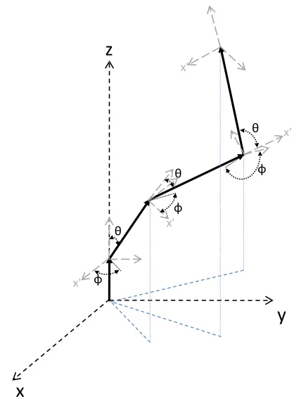
Figure 4.4 Photon propagation illustrated. Each successive scattering event causes the trajectory to rotate its local coordinate frame byθ,φ, while the global position is updated in reference to the(0, 0, 0)coordinate. . . 24

Figure 4.5 Illustration showing how the weight is reduced at each optical event. . . 25

Figure 4.6 Illustration showing how the power is integrated over an offset aperture . . . 31

Figure 4.7 Illustration showing multiple scattering and temporal dispersion. . . 37

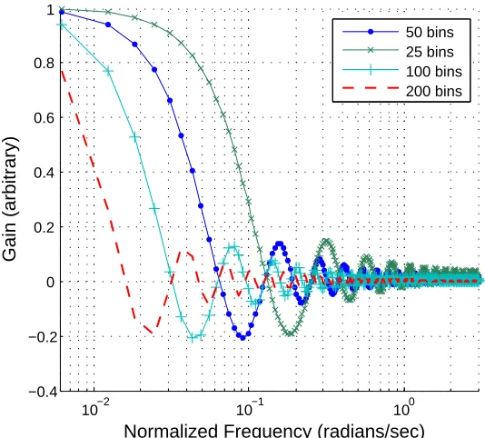
Figure 4.8 Frequency response of various windowing functions. . . 38

Figure 4.9 25 attenuation length impulse response. . . 39

Figure 4.10 Experimental on-axis beam profile. . . 40

Figure 4.11 Simulation geometry for the simulations of fixed-size polystyrene spheres . . . 41

Figure 4.12 Scattering phase function for 1µmpolystyrene spheres suspended in water . . 42

Figure 4.13 Photonator compared to published data at an optical depth of 2 - front . . . 43

Figure 4.14 Photonator compared to published data at an optical depth of 2 - side . . . 44

Figure 4.15 Photonator compared to published data at an optical depth of 5 - front . . . 45

Figure 4.16 Photonator compared to published data at an optical depth of 5 - side . . . 46

Figure 4.17 Photonator compared to published data at an optical depth of 10 - front . . . 47

Figure 4.18 Photonator compared to published data at an optical depth of 10 - side . . . 48

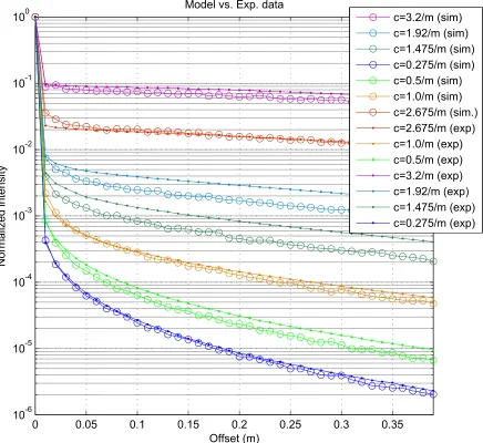
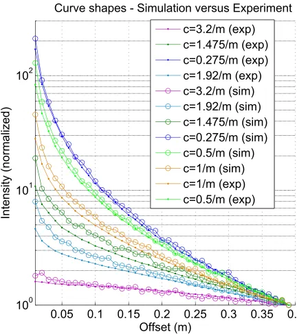
Figure 4.19 Exp. vs. Sim. for offset power. Normalized to highest power. . . 50

Figure 4.20 Exp. vs. Sim. for offset power. . . 51

Figure 4.21 Block diagram of experiment in laboratory water tank. . . 52

Figure 4.22 Gain vs. control voltage for the H6780-20 PMT used in the experiment. . . 53

Figure 4.23 PMT signal gain vs. control voltage . . . 54

Figure 4.24 Experimentally measured optical power v. turbidity of water . . . 54

Figure 4.25 Adjusted optical transmitted power . . . 55

Figure 4.26 Measured receiver FOV . . . 57

Figure 4.27 The CDF of several VSFs are plotted . . . 58

Figure 4.28 Experimental data (red) versus several simulations and Beer’s Law. . . 59

Figure 5.1 Petzold VSFs . . . 63

Figure 5.2 Offset geometry for receiver/transmitter misalignment . . . 65

Figure 5.3 Gaussian beam diverged illustration . . . 67

Figure 5.4 Gaussian beam geometric power loss . . . 69

Figure 5.5 Results of Fig. 5.4 plotted with a logarithmic y-axis. . . 70

Figure 5.6 Geometric loss from Gaussian beam spreading . . . 71

Figure 5.8 Harbor I - 1 inch aperture received normalized power. . . 77

Figure 5.9 Harbor I - 2 inch aperture received normalized power. . . 78

Figure 5.10 Harbor I - 3 inch aperture received normalized power. . . 79

Figure 5.11 Harbor I - 4 inch aperture received normalized power. . . 80

Figure 5.12 Harbor II - 8mm aperture normalized power. . . 81

Figure 5.13 Harbor II - 1in aperture received normalized power. . . 82

Figure 5.14 Harbor II - 2in aperture received normalized power. . . 83

Figure 5.15 Harbor II - 3in aperture received normalized power. . . 84

Figure 5.16 Harbor II - 4in aperture received normalized power. . . 85

Figure 5.17 Harbor III - 8 mm aperture normalized power. . . 86

Figure 5.18 Harbor III - 1in aperture normalized power. . . 87

Figure 5.19 Harbor III - 2in aperture normalized power. . . 88

Figure 5.20 Harbor III - 3in aperture normalized power. . . 89

Figure 5.21 Harbor III - 4in aperture normalized power. . . 90

Figure 5.22 Harbor I - Normalized, average, received power . . . 91

Figure 5.23 Harbor II - Normalized, average, received power . . . 92

Figure 5.24 Harbor III - Normalized, average, received power . . . 93

Figure 5.25 Harbor I - Power versus FOV - 10c z . . . 94

Figure 5.26 Harbor I - Power versus FOV - 16c z . . . 95

Figure 5.27 Harbor I - Power versus FOV - 20c z . . . 96

Figure 5.28 Harbor I - Power versus FOV - 25c z . . . 97

Figure 5.29 Harbor II - Power versus FOV - 10c z . . . 98

Figure 5.30 Harbor II - Power versus FOV - 16c z . . . 99

Figure 5.31 Harbor II - Power versus FOV - 20c z . . . 100

Figure 5.32 Harbor II - Power versus FOV - 25c z . . . 101

Figure 5.33 Harbor III - power versus FOV at 10AL . . . 102

Figure 5.34 Harbor III: 16 attenuation lengths, 3.6 meters - power versus FOV . . . 103

Figure 5.35 Harbor III: 20 attenuation lengths, 4.5 meters - power versus FOV . . . 104

Figure 5.36 Harbor III 25 attenuation lengths, 5.7 meters - power versus FOV . . . 105

Figure 5.37 Harbor I received power normalized by the receiver area. . . 107

Figure 5.38 Harbor II received power normalized by the receiver area. . . 108

Figure 5.39 Harbor III received power normalized by the receiver area. . . 109

Figure 5.40 Coastal water, 8mm aperture received power. . . 111

Figure 5.41 Coastal water, 1 in aperture received power. . . 112

Figure 5.42 Coastal water, 2 in aperture received power. . . 113

Figure 5.43 Coastal water, 3 in aperture received power. . . 114

Figure 5.44 Coastal water, 4 in aperture received power. . . 115

Figure 5.45 Clear water, 8 mm aperture received power . . . 116

Figure 5.46 Clear water, 1in aperture received power . . . 117

Figure 5.47 Clear water, 2in aperture received power . . . 118

Figure 5.48 Clear water, 3in aperture received power . . . 119

Figure 5.49 Clear water, 4in aperture received power . . . 120

Figure 5.50 Scattering orders plotted versus received power . . . 123

Figure 5.52 Harbor II - 16c zScattering Histogram . . . 126

Figure 5.53 Harbor II - 20c zScattering Histogram . . . 127

Figure 5.54 Scattering histogram of received photons for Harbor II water at 25c z. . . 128

Figure 5.55 Harbor II - 10c zscattering histogram normalized by max FOV. . . 129

Figure 5.56 Harbor II - 16c zscattering histogram normalized . . . 130

Figure 5.57 Harbor II - 20c zscattering histogram normalized by max FOV. . . 131

Figure 5.58 Harbor II - 25c zscattering histogram normalized . . . 132

Figure 5.59 Harbor water average scattering histogram - 10c z . . . 133

Figure 5.60 Harbor water average scattering histogram - 16c z . . . 134

Figure 5.61 Harbor water average scattering histogram - 20c z . . . 135

Figure 5.62 Harbor water average scattering histogram - 25c z . . . 136

Figure 5.63 Zoomed view of Fig. 5.59 . . . 137

Figure 5.64 Harbor II frequency response, 25c z . . . 139

Figure 5.65 Harbor I water frequency response at 16 attenuation lengths (dr x/t x of 14.5 meters). . . 140

Figure 5.66 Harbor I water frequency response at 20 attenuation lengths (dr x/t x of 18.2 meters). . . 141

Figure 5.67 Harbor I water frequency response at 25 attenuation lengths (dr x/t x of 22.7 meters). . . 142

Figure 5.68 Harbor II water frequency response at 16 attenuation lengths (dr x/t x of 7.3 meters). . . 143

Figure 5.69 Harbor II water frequency response at 20 attenuation lengths (dr x/t x of 9.1 meters). . . 144

Figure 5.70 Harbor II water frequency response at 25 attenuation lengths (dr x/t x of 11.3 meters). . . 145

Figure 5.71 Harbor III water frequency response at 16 attenuation lengths (dr x/t x of 3.6 meters). . . 146

Figure 5.72 Harbor III water frequency response at 20 attenuation lengths (dr x/t x of 4.5 meters). . . 147

Figure 5.73 Harbor III water frequency response at 25 attenuation lengths (dr x/t x of 5.7 meters). . . 148

Figure 5.74 Illustration showing the concept of offset received power. . . 150

Figure 5.75 Radial power calculation illustration . . . 150

Figure 5.76 Harbor I misalignment, 10c z . . . 155

Figure 5.77 Harbor I misalignment, 16c z . . . 156

Figure 5.78 Harbor I misalignment, 20c z . . . 157

Figure 5.79 Harbor I misalignment all, 16c z . . . 158

Figure 5.80 Harbor I misalignment all, 20c z . . . 159

Figure 5.81 Harbor II misalignment, 10c z . . . 160

Figure 5.82 Harbor II misalignment, 16c z . . . 161

Figure 5.83 Harbor II misalignment, 20c z . . . 162

Figure 5.84 Harbor II misalignment all, 16c z . . . 163

Figure 5.85 Harbor II misalignment all, 20c z . . . 164

Figure 5.87 Harbor III misalignment, 16c z . . . 166

Figure 5.88 Harbor III misalignment, 20c z . . . 167

Figure 5.89 Harbor III misalignment all, 16c z . . . 168

Figure 5.90 Harbor III misalignment, 20c z . . . 169

Figure 6.1 Receiver/transmitter geometry . . . 177

Figure 6.2 The ratio of k and c vs. the water albedo . . . 180

Figure 6.3 Diffuse attenuation coefficient vs. wavelength . . . 181

Figure 6.4 World map showing water conditions. . . 182

Figure 6.5 Solar radiance angular distribution at water depths . . . 184

Figure 6.6 Modifiedb value geometry . . . 188

Figure 6.7 Differential modified b value . . . 190

Figure 6.8 Simulated and modeled power loss for Harbor II water . . . 192

Figure 6.9 MAPE for Harbor waters . . . 193

Figure 6.10 Simulated power versus distance for PMT and PD link. . . 197

Figure 6.11 Simulated SNR versus Distance . . . 198

Figure 6.12 Bit error rate versus distance for PMT and Photodiode based links. . . 199

Figure 6.13 Block diagram of polarization modulation system using two diode laser and two orthogonal detectors. . . 200

Figure 6.14 Bit error rate versus SNR of the received data for both a single laser OOK system, and the PolModSK system. Also shown is the system performance using a UMTS Turbo Code. . . 201

Figure 6.15 Bit error rate versus the attenuation length of the systems (for a fixed distance of 3.66 m). Also shown is the system performance using a UMTS Turbo Code. . 201

Figure 6.16 Degree of polarization (DOP) versus transmission distance for several different water types. . . 203

Figure 6.17 Degree of polarization (DOP) versus received power for various water types. . . 203

Figure 6.18 Diagram showing the retroreflection process. . . 204

Figure 6.19 Experimental block diagram for MRR communication system. . . 206

Figure 6.20 Block diagram of transmitter for the MRR communication system. . . 206

Figure 6.21 Receiver diagram for MRR system. This was implemented in software in MATLAB.206 Figure 6.22 Cross section diagram of a MEMS modulating retroreflector. The device can be used for ultra-low power underwater optical communication. . . 207

Figure 6.23 MRR optical spectrum. . . 207

Figure 6.24 Top-down picture of the MRR. The small squares surrouding the four central squares are 144 indvidual modulators. . . 208

Figure 6.25 Mounted view of the MRR with interrogating laser. . . 209

Figure 6.26 View of the MRR interrogating system. . . 210

Figure 6.27 Frequency response of the (green) high-power amplifier, full system (red) and the interrogating laser and detector (blue). . . 210

Figure 6.28 Bit error rate measurements for the MEMS MRR compared with the attenuation length and received optical power. . . 211

Figure 6.30 Required transmit power to achieve 5µW of received power at the receiver. Plot shows required power at various water conditions, and various distances between the interrogator and the MRR. This assumes perfect alignment and

that the MRR is normal to the interrogating beam. . . 214

Figure 6.31 System block diagram for LED-based passband communication system using software defined radio. . . 215

Figure 6.32 Picture of one of the SDR transceivers. Image shows the PD receiver and LED transmitter, along with the USRP digitizer. . . 216

Figure 6.33 Theoretical and experimental BER versus SNR system performance . . . 217

Figure 6.34 Experimental BER versus attenuation length system performance . . . 218

Figure 6.35 Throughput for the two sets of LED-based network links. . . 219

Figure 6.36 Network latency for the two sets of LED-based network links. . . 220

CHAPTER

1

Introduction

Comprehensive ocean observation is of great interest to the scientific, industrial and military

com-munities. Security concerns, weather monitoring, and ocean commerce all require sensing of the ocean environment. The difficulty is that such measurements can be expensive, dangerous, and

quite difficult to make. Any sensor will require some form of communication, and thus underwater

communication between mobile ocean systems is of great interest. The limited propagation distance

of RF frequencies[1]and low datarate of acoustic communication leave optical communication as a

viable alternative for low-latency, high datarate communication in our oceans. By taking advantage of

the “blue/green” optical window in ocean water, underwater optical communication systems can

utilize low cost optical sources, like diode lasers[2]or LEDs[3].

Previous work has demonstrated the viability of such systems in actual ocean environments[4, 5],

along with experimental results at various datarates and turbidities[6, 7, 8, 9]. These systems are all operated in a fixed laboratory environment, or utilize LEDs as transmitters to ease the pointing and

tracking requirements inherent in optical communication systems. These systems are also either simplex (one way) communication systems or utilize two sets of transmitters and receivers for duplex

communication[10, 11]thereby increasing complexity and system power requirements. Another

option for low power optical communication is the use of a modulating retroreflector[12, 13]to

eliminate the need for an optical source at one of the endpoints.

With the overarching goal of comprehensive ocean observation, this dissertation will focus on

the design and development of underwater freespace optical communication systems, with experi-mental, theoretical, and simulated performance results for various systems. Specifically, a numerical

validated. Secondly, various communication scenarios are simulated and analyzed. Thirdly, design

considerations for constructing underwater optical communication systems are discussed, and

theo-retical link budgets are developed to aid in design. Finally, experimental results of various systems are discussed and compared with simulated and theoretical performance metrics.

The goal of this research is to present several tools to the underwater optical communication system designer. These are a validated numerical simulation for computing the received optical signal power, along with theoretical calculations for computing the SNR of the received signal. This helps solve the problem of the difficulty of building and testing actual systems in ocean envi-ronments in order to get operational data. This will enable better systems for ocean observation.

The following chapters will first detail the current state of the art of underwater optical

commu-nications. Secondly, we will discuss the physical interactions of light and water in the ocean. Third,

we will detail the design and validation of the Monte Carlo numerical simulation, Photonator, then use the simulation tool to simulate various communication scenarios. Finally, we will develop a

CHAPTER

2

Overview of the State-of-the Art

Underwater communication has a lengthy history starting with Leonardo da Vinci observing, “If you

cause your ship to stop, and place the head of a long tube in the water and place the outer extremity to your ear, you will hear ships at a great distance from you.[14]”. He wrote this in 1490, but it wasn’t till the proliferation of submarine warfare during World War I that research into sonar systems became

necessary, and Paul Langevin created a device for detecting the noise from moving submarines in 1915. The first useful device for communication underwater was the underwater telephone, an acoustic

device developed in 1945[15]. World War II and the Cold War caused great advances in submarine

communication due to the creation of the computer[16].

2.0.1 Freespace Optical Communication

Freespace optical communication (FSOC) dates back to the ancient Romans using mirrors for sending optical signals between distant outposts. Alexander Bell also used a free-space optical transmission

scheme to encode a voice signal and transmit it to a receiver over six hundred feet away[17]. The

creation of the laser in the 1960’s, along with advances in the area of RF communication, fueled a rapid deployment of fiber optic networks and advances in space communication systems. Along this

same time, the military proposed systems for freespace communication between submarines[18, 19]

or between satellites and submarines[20].

The end of the Cold War saw a reduction in the interest in space-to-submarine communication,

while commercial telecommunication needs spurred increased research into terrestrial optical

optic community allowed rapid increases in datarates and communication distances for terrestrial

systems[21]. More recently, though, the proliferation of unmanned underwater vehicles, the desire

for comprehensive ocean observation, and the need for command and control of these devices have lead to increased research interest into underwater communication systems.

2.0.2 Underwater Freespace Optical Communication

Recent advances in semiconductor light sources, including blue/green LEDs[3]and diode lasers[22], coupled with the need for ocean exploration and environmental sensing, have spurred research into

underwater freespace optical communication. Long range satellite-to-submarine communication

links[16]have been passed over in favor of shorter range, lower power, low cost systems to be placed

on autonomous vehicles or sensor nodes[5, 11]. Practically speaking, using LEDs as a transmitting

light source is most often used for deployable systems due to the ease of pointing and tracking. The transmitter bandwidth of these devices is somewhat limited, however, with a maximum implemented

datarate of 10 Mbps reported by Farr[5], though for terrestrial applications, datarates as high as 80 Mbps[23]have been reported by utilizing analog filtering to change the pulse shape. Digital filtering

can also be used[24]. Simpson demonstrated a 5 Mbps LED link at 7.3 meters, along with

forward-error correction capabilities[25]. Doniec demonstrated a deployed system operating at 1.2 Mbps at

30 meters, though the water quality was not quantitatively measured[10, 11]. Anguita demonstrated

a LED based receiver/transmitter system operating up to 2 Mbps over short distances (2 meters), and

based on the IEEE 802.15.4 standard for wireless personal area networks[7].

Laser-based underwater links have been explored since the 1970’s[26, 18, 19], with the

measure-ments of Snow[27]showing the first experimental results with a 7 Mhz square wave propagating over

18 attenuation lengths (-78 dB extinction) at 30 meters distance, and a 100 Mhz signal propagating 45

meters with an attenuation length of 5 m/m ( -21 dB extinction). Green wavelengths, between 514 nm

and 532 nm were used. Hanson holds the current record for datarate, with a 1 Gbps link established

in a 2 meter test tank[6]. The link ran error free up to 8 attenuation lengths and showed no signs of limitation due to inter-symbol interference or pulse spreading due to scattering. Jaruwatanadilok also

found, through complex analytical modeling, that the channel was very broadband with over 6 GHz of

bandwidth[28]. Mullen also verified experimentally the propagation of>1 Ghz RF modulated signals in the underwater channel[29].

More recently, Mullen et al. at the Patuxent River Naval base have made detailed measurements of

the scattering phase function of Maalox[30]and compared them with ocean scattering phase

func-tions. It was found that Maalox closely approximates the scattering phase function of natural waters

(though, not as well for small angles, see Fig. 3.2 on page 12). Thus Maalox provides a convenient and

suitable material to control the amount of scattering in laboratory experiments. Based on underwater

to an optical communication system by Cochenour et al.[8]and later expanded[32]. This allowed greater spectral efficiency, since high-order modulation formats could be used. Additionally, links

up to 5 Mbps were established at attenuation lengths up to 8 m/m in a short (3.66 meter) tank. The

work done by Cochenour et al.[33]compared experimental results to an approximate analytical

scat-tering function with close agreement. The model was then used to predict link performance at large

distances, which showed that Beer’s Law exponential power loss does not hold for large attenuation lengths as scattered light is captured by the receiver. Experimental results of the power loss versus

attenuation length were presented by Cochenour[34], which examined the de-polarization of the

light as it propagated. Using nigrosin dye with the Maalox allows the absorption to be controlled independent of the scattering, thus allowing the the albedo of the water to be changed to better match

ocean properties.

Some authors have also considered using the scattering nature of ocean water as an advantage

by attempting non-line-of-site (NLOS) communications[35]. By using the sea surface as a diffuse

reflector, pointing and tracking (P&T) issues could potentially be avoided, though the technical hurdles in such an implementation are many. Light attenuation in seawater is severe, so diffuse

reflection would limit the amount of photons at the receiver. Ultraviolet “solar-blind” underwater

communication has also been studied in theory by Kedar[36], while transmission lengths are very

short ( 10 meters), operation in shallow water with very wide field-of-view receivers is feasible due to

the lack of background solar noise (see Section 6.2.1).

Another area of research is the use of a retro-reflecting modulator for underwater optical commu-nication (see Section 6.7.2 on page 204). This would allow the transmitting device to operate at lower

powers since the high power optical beam is generated by the receiving, or interrogating, system.

Mullen showed a technique for suppressing backscattering from such a communication device[31],

while we experimentally demonstrated that using such a device can be used for communication at

several attenuation lengths with a low power laser source (20 mW)[12, 13].

Finally, the propagation of coherent light was explored by Hanson[37]by studying the effects of

light propagating over a turbid path and coupling that light into a single-mode fiber. The received

optical signal could then be used with modern telecommunications equipment to simplify the design

requirements for optical modem technology. Results showed the fiber coupling efficiency was directly related to the beam size versus the coherence length, and the effects of turbulence are reduced as the

beam size is reduced.

2.0.3 Monte Carlo Model of Terrestrial Light Transportation

Monte Carlo simulations have been used in modeling terrestrial optical freespace communication

scattering phase function underwater, in that it is non-isotropic and highly forward peaked. Much

can be learned from these techniques. Older implementations used the Henyey-Greenstein scattering

function as a good approximation of scattering in clouds. This function is described by,

e

βHG(g;ψ) =

1 4π

1−g2

(1+g2_{−2gcos(ψ))}3/2 (2.1)

whereβeis the scattering phase function (described below) that is dependent on the scattering angle,

ψand parameterg. This parameter controls the amount of forward versus backward scatter. This

parameter fails to account for the significant forward scattering at very small angles in the underwater

environment and backscattering at very large angles. Several modifications of this function have been proposed to better match Mie theory. Figure 2.1 below shows an example of several scattering phase

functions.

Figure 2.1: The dotted line is the measured phase function from water. The solid line is for cirrostratus

cloud at 550 nm. The+signs are human liver tissue at 635n mand the dashed line is for atmospheric

haze at 550n m[40].

For known particle size distributions, Mie theory can be used to analytically compute the scattering

phase function[36, 39]. This calculation usually has to be computed and stored as a look-up table

in order to make the simulation computationally efficient[41]. The Mie scattering phase functions

can easily be used in atmospheric simulations as the atmospheric constituents are known and well defined. The task is more difficult for the underwater environment where the constituents are widely

varied. For example, there can be wildly different scattering from suspended sediment that can

2.0.4 Monte Carlo Modeling of Light Underwater

The propagation of light underwater has been traditionally studied for its effects on plant and animal

life, not for optical communication. In the former case, the illuminating source is the sun, and

the photons are tracked through the air/water interface and as they move downward through the

water. As these photons propagate, they are either absorbed or scattered in another direction. To

determine the amount of absorption, either to determine heating or photosynthetic reactions, Monte Carlo simulations have been used to track the photon interactions through the water volume. These

simulations typically use a “bin” method, where each interaction’s location and angle is recorded so

the radiant energy through the whole volume can be determined[42, 43]. These measurements are

compared with data taken from instruments that can directly measure the upwelling and downwelling

irradiance of the lightfield underwater.

Monte Carlo simulations of directional optical transmitters to optical receivers are not very com-mon due to their computational complexity. Many aspects of downwelling or upwelling irradiance

calculations make them easy to compute, however they provide limited information in a

communica-tions context, where the field of view and receive aperture are both limited. They can, however, aid in the calculation of background noise, as discussed in Section 6.2.1. A few Monte Carlo models for

simulating optical communication have been mentioned in the literature. Laux[30]describes a MC

model used to compare against experimental tank data. Hanson[6]utilized a MC model to compare

against a high-bandwidth communication experiment, and extrapolate the results to longer distances.

Jaruwatanadilok[28]mentions, but does not describe, using a MC model to compare against

the-oretical calculations of channel bandwidth. More recently, Li[44]developed a semi-analytic MC

simulation, which they verified using experimental channel measurement data from Mullen et al[29],

and then used to make channel bandwidth estimations. While the methods used have been discussed, to this author’s knowledge, none of the previously mentioned authors have made their source-code

available for use or analysis.

2.1

Conclusion

In summary, underwater freespace optical communication draws from a rich history of various

disciplines: optical communication, freespace optical, and underwater communication, along with laser development and mathematical modeling. The area has not been as widely explored as terrestrial

or space freespace optical communication, but recent advances in low-cost light sources, and more

interest in ocean observation, have spurred current research. Much work still needs to be done in the area of modeling and system design, which this research addresses, along with continued efforts

to improve the bandwidth of detectors and sources and output power of visible wavelength optical

CHAPTER

3

Light Underwater

The interaction of light and water is quite complicated. Not only does it deal with the complex subject

of light interacting with matter, but also deals with the complex nature of the ocean environment. This chapter will try and distill the most important aspects of this interaction as it applies to underwater

freespace optical communication. For a more complete view of the subject the works of Mobley [40, 45]and Spinrad[46]are very useful resources.

In general we will address the issues of optical absorption and scattering in the water, as these two

factors contribute to power loss between an optical transmitter and a receiver. Other effects, such as

photoluminescence, will not be considered.

3.1

Characterizing Light in Water

When considering a differential volume element of water of width∆r, and arbitrarily small height

and length, the amount of light entering the volume equals the amount of light leaving the volume,

less any absorption loss in the volume. A portion of light leaving the volume will retain the same

propagation direction, while the rest will be distributed into other directions. This is illustrated in Fig. 3.1 and based off the work by Mobley[40].

If the the differential volume of water illuminated with a spectral radiant power ofΦi,Φa is the

absorbed power,Φs is the total scattered power in all directions, andΦt is the transmitted power.

Note that all of these values are wavelength dependent, but theλdesignation has been dropped for

∆𝑟

Φ

𝜆

Φ

𝜆

Φ

𝜆

Φ

𝜆

ΔΩ

𝜓

𝜑

Figure 3.1: Geometry of the inherent optical properties of water, from Mobley[40].

Φi(λ) =hc

λ

N

∆λ (3.1)

wherehc/λis the energy of a photon of wavelengthλ,N is the number of photons observed per

second, and∆λis the wavelength range of the observation (or the bandwidth of a filter in a detector).

The units of spectral radiant power are W nm−1_.

We will define the absorptance as

A(λ) =Φa

Φi (3.2)

the transmittance as

T(λ) =Φt

Φi (3.3)

and the ratio of scattered power as

B(λ) =Φs

Φi. (3.4)

If we divide the quantities above by the distance, ∆r, as it approaches zero, then the values

above are reduced to coefficients which measure loss per unit distance. These are referred to as the absorption coefficient

a(λ) =d A(λ)

and the scattering coefficient

b(λ) =d B(λ)

d r (3.6)

where both are in units ofm−1_{, sinceB(λ)andA(λ)are unit-less ratios. Additionally, the total loss is}

defined as theattenuation coefficient,c, where

c=a+b (3.7)

which also has units ofm−1_{. An additional helpful value is the single scattering albedo,ω} 0,

ω0=

b

c (3.8)

which defines are ratio of scattering loss to total loss. This is a helpful term when comparing various

water types, as we will see in future chapters. This value is in the range of values from 0 to 1 (expressed

as[0, 1]), with natural waters having values from around 0.25 for clear ocean water to over 0.8 for

turbid harbor waters. A completely scattering medium would have a value of 1, while a medium with

no scattering and only absorption loss would have a value of 0.

3.2

Absorption

The absorption in natural waters can be difficult to separate from scattering when taking

measure-ments. Not only does pure water absorb some amount of the optical energy, but the particulate matter in these waters can be even more absorptive. Suspended materials that contribute to absorption

include “colored dissolved organic material” (CDOM) and phytoplankton. CDOM absorbs more at

shorter wavelengths, while phytoplankton absorbs strongly in the blue and red wavelength regions due to the chlorophyll concentration[47].

3.3

Scattering

Light scattering is due to photon interactions with the water molecules, particulate matter, and other

dissolved substances in the water. The beam loss from scattering, shown asΦsin Fig. 3.1, is dependent

on the angle,ψ, of deviation from the incident beam direction. Since the scatterers in ocean water

are randomly distributed the radial angle,ϕof scattering is symmetric, shown by the annular ring in

Fig. 3.1. The angular distribution of scattering, called the volume scattering phase function, is defined as

β(λ,ψ) = lim

∆r→0∆Ωlim→0

Φs(ψ;λ)

which is the limit of light scattering out of volume∆rinto the solid angle∆Ωin directionψ, as both go to zero. The units ofβ(λ;ψ)are m−1_sr−1_{. By integratingβover all angles, we arrive at an expression}

forb(λ), given by

b(λ) = Z

4π

β(ψ;λ)dΩ =2π

Zπ

0

β(ψ;λ)sinψdψ (3.10)

since the radial scattering angle is symmetric, the integration on that axis reduces to 2π, and the polar scattering angle is in the range[0,π].

If the volume scattering phase function,βis normalized by the scattering coefficient,b, then

we arrive at the volume scattering phase function,βe, which expresses the angular probability of

scattering as a probability density function (PDF)

e

β(λ;ψ) =β(λ;ψ)

b(λ) . (3.11)

The volume scattering phase function is used to choose scattering angles for the numerical MCNS

simulation discussed in Chapter 4. In practice, measuring the volume scattering function is very difficult due to the large dynamic range needed for the measurement device.

3.4

Analytical Models

A simple approach to the solution of the scattering problem is available for small spherical particles

(radius<λ). For larger spherical particles the Lorenz-Mie solutions of Maxwell’s equations provide

a very useful result. However, analytically modeling the scattering phase function is fraught with problems in many real world applications. Not only are the measurements of the volume scattering

functions extremely difficult to measure, they also require expensive, time consuming, and dangerous

sea voyages to measure actual ocean environments. Many different types of analytical phase functions

have been used over the years. The Henyey-Greenstein (HG) function has been popular[41, 50], and

was originally based on interstellar dust scattering. In more recent years, the Fournier-Forand (FF)

function has been used with good agreement to actual water measurements[51, 52].

The FF model was proposed[53]as an analytic phase function based on the anomalous diffraction

approximation of Van de Hulst[54]. While still being a relatively simple, two parameter, equation, it has be benefit of being rooted in the physics of the problem instead of being a purely phenomenologi-cal model. The FF phase function assumes that the particle distributions in natural waters follow a

hyperbolic (Junge) distribution, which, in practice seems to be appropriate[55, 56], and is based upon the slope of the Junge distribution and the average real index of refraction of the particles. Recently,

Mobley et al.[51]was able to re-parameterize the FF function based upon the backscattering fraction,

10−1 100 101 102 10−3

10−2 10−1 100 101 102 103

scattering angle, degrees

phase function, sr

−

1

Maalox − A. Laux Harbor − Petzold Coastal − Petzold Clear − Petzold Maalox − Petzold Maalox − D. Grey HG, g= 0.93 Fournier−Forand Petzold Average

Figure 3.2: Comparison of various phase functions. Shown are measured phase functions from Deric Grey (Maalox)[48], Alan Laux (Maalox)[30], Petzold (Maalox and ocean water)[49], along with a Henyey-Greenstein phase function, and a Fournier-Forand phase function for the Petzold average phase function. These are plotted on a log-log plot to emphasize the effects of small angles.

90◦_{for a single scattering event (for exampleBp =0.0183 for the average Petzold scattering phase}

function). This parameterization is very helpful as it is difficult to measure the average index of

re-fraction of the particles in natural waters. Freda and Piskozub[57]compared Mobley’s approximation

with experimental data from natural waters and proposed an additional set of parameterizations that

better match the data.

When just comparing Petzold’s measured data with the FF phase function, however, a very good

fit can be made by using the parametersµ=3.5835 andn=1.10. The phase function has the benefit

of modeling both the sharply peaked forward scattering and the backscattering peak of natural waters. The FF phase function is therefore appropriate for both modeling the backscattering effects in LIDAR

and communication interference and for forward scattering used in communication. However, the

function, along with the average Petzold phase function, is shown in Fig. 3.2.

3.5

Full System View of Light Reception

When considering the loss of light over a path length,r, the attenuation coefficient can be used to

describe the total loss. Essentially, the differential path loss is integrated over the distance. If the

differential path loss is

d I

d r =−c I (3.12)

whereI is the power incident on the volume of widthd r, andcis the attenuation coefficient,a+b

with units ofm−1_{.cis negative to show that light is lost over the path. Rearranging this equation and}

integrating yields

ZI

I0

1

I d I=−c Z r

0

d r ⇒ln(I)−ln(I0) =−c r (3.13)

which, when simplified, yields the more common expression for Beers Law-type loss:

I=I0exp(−c r). (3.14)

This equation assumes that all scattered light is lost from the beam and that no multiply scattered light returns to the beam, and as such, does not take into account a receiver of finite aperture. A

modification to compensate for this effect is discussed in Section 6.4.1 on page 188. In general,

however, a full view of light loss and reception will take into account both the loss due to scattering and the gain due to photons scattering back into the central beam. This total view is considered in the

next section on the radiative transfer equation.

The exponent of Eq. 3.5 is a unit-less quantity called theattenuation length, and is the multiple of

the transmission distance and the attenuation coefficient. This quantity,c z, is often used to compare

operation of various systems, since it removes the ambiguity of distance and water conditions.

3.5.1 Radiative Transfer Equation

The radiative transfer equation expresses the conservation of energy of an underwater beam of light.

It takes into account losses and gains into the central received beam. The equation is expressed using the definitions above and the radiance of the beam

L(z,λ,φ,θ) =P(λ,z,φ,θ)

where∆Ais the area of the detector,∆Ωis the solid angle in the direction ofφ,θ, andzis the operating

depth in the ocean. The units of radiance are W m−2_sr−1_nm−1_{. Using the radiance, the radiative}

transfer equation for the simple case of a homogeneous medium, with no inelastic scattering or internal sources like bioluminescence, is

cosθd L(z;λ;θ;φ)

d z =−c(z,λ)L(z;λ;θ;φ) + Z

4π

β(z;λ;θ0→θ;φ0→φ)L(z;λ;θ0;φ0)dΩ0 (3.16)

whereL(z;λ;θ;φ)is the radiance at depthzin directionθ,φ. The first term on the right,−c(z,λ)L(z;λ;θ;φ) is the Beer’s Law loss, and the 2nd term is the gain from light scattering from angleθ0_,φ0_{into direction}

θ,φ. Even in this simplistic case, this equation is difficult to solve. The Monte Carlo simulation tool in Chapter 5 on page 62 presents a way to solve this equation for an optical transmitter and receiver.

3.5.2 The Diffusion Length

The diffusion length,Ld, introduced by Weisskopf[58]is a useful term when determining whether a

system is operating in low to moderate attenuation lengths or at high attenuation lengths. Its equation

is

Ld =

1

b(1− 〈cosθ〉) (3.17)

where〈cosθ〉is the average scattering cosine,g, given as

〈cosθ〉=2π

Z π

0

e

β(θ)cosθsinθdθ. (3.18)

This equation is simply the average of the volume scattering phase function, such that〈cosθ〉

represents the point where half of the total scattering happens at angles above〈cosθ〉and half below.

Eq. 3.17 is derived by calculating the total average length over which a photon propagates along

the initial direction, after an infinite number of scattering events. Sinceb−1_{describes the average}

length a photon travels, the distance which a photon moves along the initial direction vector after

the first scattering event isb−1_+b−1_{cosθ, whereθ is the azimuthal scattering direction. After the}

second scattering event, this distance then becomesb−1_+b−1_cosθ+b−1_cos2_{θ, and so forth. On}

average, each scattering event addsb−1_{〈cosθ〉to the total distance. This equation}

Ld =b−1+b−1〈cosθ〉+b−1〈cosθ〉2+...=b−1

∞ X

i=0

〈cosθ〉i (3.19)

is a geometric sum, which, since〈cosθ〉is<1, reduces to the result in Eq. 3.17.

Table 3.1: Albedo, average cosine, and diffusion attenuation length for the three Petzold water types.

Turbid Coastal Clear

ω0 0.83 0.55 0.25

〈cosθ〉 0.92 0.94 0.87

c LD 15.1 30.3 30.7

thick”. If the medium is isotropic, then the diffusion length will simply beb−1_{. However, as the}

scattering phase function, βe(θ)becomes more peaked in the small angles, the diffusion length

increases. Essentially, it takes longer before the number of photons scattering backwards, equals those

scattering forward. While photons still continue to move along the incident direction,on averagethe

forward motion has stopped by distanceLd.

By looking at the diffusion length in terms of the number of attenuation lengths, as developed by

Cochenour and Mullen[60], the following equation is derived

c LD=ω_o−1

1

1− 〈cosθ〉 (3.20)

whereωois the albedo of the water. This number ranges from 0.25 for clear ocean waters to 0.83 for

turbid harbor waters. The average scattering cosine,〈cosθ〉, for Petzold’s harbor water scattering

phase function ranges from 0.87 to 94. This number is typically greater than 0.90 for natural waters, and is 0.924 for the average Petzold scattering phase function. For the three Petzold water types, the

diffusion length is presented in Table 3.1.

Based on Table 3.1 it is clear that Coastal and Clear water types maintain their forward scattering motion over a very long distance when compared to harbor water. At 30 attenuation lengths, the

optical source will be attenuated by more than thirteen orders of magnitude. This makes it very difficult to experimentally measure this type of waters at the point they begin to significantly diverge

from Beer’s Law, and similarly difficult to simulate this behavior. In this sense, harbor water types

prove to be much more “interesting” from a scattering perspective. Thus, most of the work in this thesis is focused on various Harbor water conditions, though results are presented for Clear and

Coastal waters to illustrate their differences.

3.6

Conclusion

In conclusion, the interaction of light and water is quite complicated, and depends highly upon

both the wavelength of the light and the constituents of the water. Decades of research have been devoted to understanding these interactions, especially in regards to biological effects and underwater

imagining, such as LIDAR. While point-to-point communication is a relatively small aspect of this

Light loss between the transmitter and receiver is governed both by absorption of the photons by

the water molecules, suspended particulate matter, and dissolved materials and scattering.

Chloro-phyll in phytoplankton, along with CDOM are two chief absorbers of visible wavelengths in the under-water channel. These depend highly on the location and depth an underunder-water optical communication

system is operating. Scattering affects also play a large part in underwater optical communication,

as they contribute to temporal dispersion (elongation of the path length that photons travel) and to power loss as photons are scattered away from the receiver aperture. Scattering is also highly

dependent on suspended particulate matter and the water itself, and is difficult to model due to the

variability of the scattering phase functions chiefly at small angles. Both theoretical and phenomeno-logical models can be used in simulations and analytical calculations of power loss in communication

systems. Additionally, looking at the scattering characteristics of the water can tell us important

aspects of the power loss models, as past a certain distance, the diffusion length, the propagation of the light is no longer predominantly collimated and forward scattering. As we will see in later chapters,

the diffusion length can be a useful indicator for a change in the shape of the power loss curves in highly scattering environments, such as Harbor water. Finally, for many waters types the Beer’s Law

loss model works well to characterize the loss of signal power over a given distance. This model is

CHAPTER

4

Simulation of the Underwater Lightfield

Since field testing is both costly and time consuming, an important aspect of system design is

the ability to predict the system’s performance prior to construction and testing. While various approximations and analytical models of the underwater light-field exist, these often do not take

into account the specific needs for optical communication or can be inadequate for determining

optimal system performance. For example, while Beer’s Law (see Eq. 3.5 on page 13) provides a convenient equation for determining the channel loss, it can severely underestimate the power of

the light-field in highly turbid environments, thereby underestimating the system’s performance in

such an environment. Another example would be analytical models which employ the small angle approximation. While these models are very convenient for rapid calculation of the light-field power,

they cannot yield correct answers for extreme pointing angles or non-line of sight communication.

Additionally, typically these models do not take into account time resolution and thereby make it difficult to determine the channel bandwidth of the underwater optical communication channel.

In order to fill some of the gaps left by other kinds of channel models, a Monte Carlo numerical simulation (MCNS), “Photonator”, is presented for calculating the underwater light-field, specially for

optical communication systems. The simulation is useful both in terms of the underlying simplicity

of the simulation and the public presentation and availability of the software for general use.

4.1

Overview of Monte Carlo Numerical Simulation

Monte Carlo numerical simulation (MCNS) uses random sampling to arrive at an approximate answer

problem. Put another way, a MCNS approximates a complex probability distribution function (PDF)

through random sampling of known, exact, simpler PDFs. For our particular problem, the underwater

light-field, a solution to the PDF of the light-field on the receiver is desired. This can be computed using approximate formulas to arrive at an exact solution to these formulas, or a large number of

photon trajectories can be computed, each using known PDFs for scattering lengths and volume

scattering functions. These photon trajectories can be summed to approximate the light-field at the receiver. In the area of computer graphics, this method is generally termed “ray tracing”, due to the

tracing of individual rays of light from source to receiver. Mobley[40]describes the Monte Carlo

method as knowing, “the probability of occurrence of each separate event in a sequence of events, then we can determine the probability that the entire sequence of events will occur.”

While MCNS requires a great deal of computational power, the Moore’s Law-type increase in

computation power makes the method more and more feasible as time progresses. Additionally, the conceptually simple methodology makes it accessible to students and researchers who do not

possess a background in mathematics, required for many of the analytical models. The simulation is

constructed according to common methods described in many publications[61, 62, 63, 64, 65, 66, 67,

68, 43, 40, 30]. Especially helpful references include that of Mobley[40], Leathers[62], and Wang[65].

4.2

Simulation Assumptions and Approximations

While the number of assumptions about the behavior of the MCNS were kept to a minimum, there

are still several assumptions that were made and need to be noted. These are listed below, along with explanation:

• Homogeneous medium - Photonator MCNS assumes that the simulation medium is homo-geneous, meaning that scattering and absorption are uniform throughout the volume of the

environment.

• Elastic scattering (no Raman, etc.) - All scattering is assumed to be elastic, meaning there are no shifts in wavelength, only direction.

• Random number generator produces sufficiently independent uniform random numbers - No computational random number generator is perfect, and will eventually repeat the random

string of numbers. In the MCNS the random number generator is seeded with a new seed for

each time the simulation is run.

• Simulation boundaries are perfectly absorbing - For open water simulations, photons that

propagate backwards past the transmitter plane are terminated.

• No photons propagate past the receiver plane, back, and then across it again (no 3x

• Sufficient number of photon packets are collected to form an accurate estimation of the total

probability from transmitter to receiver - by randomly sampling a discrete distribution to

approximate a continuous distribution, it is assumed that after a certain point the discrete approximation begins to approach the continuos approximation. This assumption can be

tested using the Central Limit Theorem.

Other assumptions, when made, are noted. Any assumptions that were made were usually chosen not from convenience but from necessity - whether this was computational complexity necessity or

simply based on the numerical method chosen.

4.3

Mechanics of the Photonator Simulation

The simulation is divided into three major parts: initial conditions, photon propagation, and photon

reception. Each part will be discussed below. The three section correspond to three aspects of the source code in Appendix B on page 235. The two major processes, transmission and reception, are

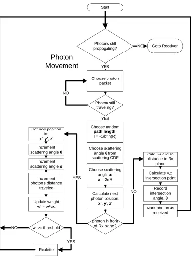
illustrated via a flowchart in Fig. 4.1 and Fig. 4.2. Photons that are propagated in the transmission

process are passed to the receiver process, once all photons have been terminated or received, for processing into irradiance and power measurements on the receiver plane.

4.3.1 Initial Conditions

The simulation initial conditions determine the type of environment, the type of light source, and

the receivers that will be simulated. The simulation geometry uses a cartesian coordinate system

where the receiver plane is situation on the x/y-plane at a fixed point along the z-axis. Any photons

that cross the x/y-receiver plane are marked as received and their x/y location, and arrival angle are recorded. While the receiver(s) is always on the x/y plane, the initial location and incident angles of the light source is not limited.

Light source definition

Each photon packet is determined by itsx,y, andz location and the projection of a unit vector, in

the direction of propagation, projected on thex,y, andzaxes. These projections, commonly called

“direction cosines” determine the direction of propagation of the photon and reduce the need for time

consuming and complex trigonometric calculations. The photon direction vector is projected onto the x,y and z axis of the Cartesian coordinate frame. These projections, are illustrated in Fig. 4.3 and

are defined by,

Choose photon packet Photons still propogating? Photon still traveling? Choose random

path length: l = -1/b*ln(R)

Choose scattering angle θ from scattering CDF

Choose scattering angle ø:

ø = 2πR

Calculate next photon position:

x’, y’, z’

photon in front of Rx plane?

NO YES NO YES Goto Receiver NO NO

Set new position to:

x’, y’, z’

YES Increment

scattering angle θ

Increment scattering angle ø

Increment photon’s distance

traveled

Calc. Euclidian distance to Rx

plane

Calculate y,z intersection point

Record intersection

angle, θ

Mark photon as received

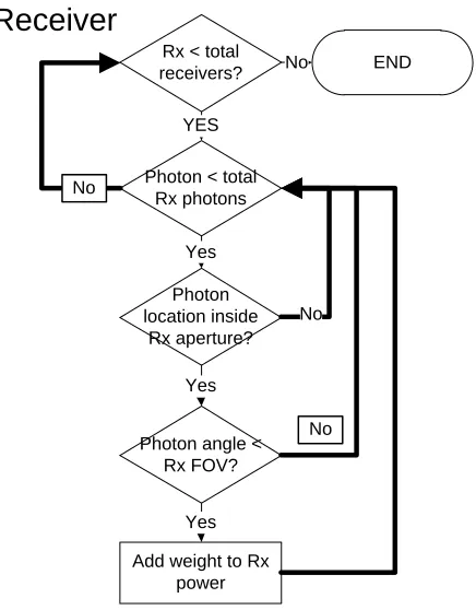
Rx < total receivers?

Photon < total Rx photons YES END Photon location inside Rx aperture?

Photon angle < Rx FOV? Yes Yes No No No No

Receiver

Photon

Movement

w’ = w*ω0

w’ >= threshold

Roulette

YES

Start

Figure 4.1: Flowchart showing basic process for transmitting photons from the transmitter to receiver. The flowchart starts at the top and moves downward. Once all the photons have been terminated, the process is passed to the receiver, illustrated in Fig. 4.2

Choose photon packet Photons still propogating? Photon still traveling? Choose random

path length: l = -1/b*ln(R)

Choose scattering angle θ from scattering CDF

Choose scattering angle ø:

ø = 2πR

Calculate next photon position:

x’, y’, z’

photon in front of Rx plane?

NO YES NO YES Goto Receiver NO NO

Set new position to:

x’, y’, z’

YES Increment

scattering angle θ

Increment scattering angle ø

Increment photon’s distance

traveled

Calc. Euclidian distance to Rx

plane

Calculate y,z intersection point

Record intersection

angle, θ

Mark photon as received

Rx < total receivers?

Photon < total Rx photons YES END Photon location inside Rx aperture?

Photon angle < Rx FOV? Yes Yes Yes No No

Add weight to Rx power No No

Receiver

Photon

Movement

w’ = w*ω0

w’ >= threshold

Roulette

YES

Start

Figure 4.2: MCNS flowchart for the receiver process. Photons are passed from the transmitter, shown in Fig. 4.1, to the receiver to be processed.

x+ y+ z 𝜃𝑥 𝜃𝑦 𝜃𝑧 𝜇𝑦 𝜇𝑥 𝜇𝑧

Figure 4.3: Illustration of direction cosines. The blue vector is the photon trajectory direction vector, the red vectors,µx,µy,µz, are the projections of the photon’s direction vector onto thex,y, andz

µy=cos(θy) (4.2)

µz=cos(θz) (4.3)

whereθx,θy, andθzare the angles between the direction vector and the x,y, and z axis, respectively.

These three values must also satisfy the normalization

µ2

x+µ2y+µ2z=1 (4.4)

which assures that the direction vector is a unit vector.

The angular representation of a source depends on the source function[62], given byΨ0(θ,φ)and

normalized such that

Z 2π

0

Zπ/2

0

Ψ0(θ,φ)sin(θ)dθdφ=1 (4.5)

whereθ is the polar angle andφis the azimuthal angle. For most sources,φwill be symmetric, and

thus the normalization is reduced to

2π Z π/2

0

Ψ0(θ,φ)sin(θ)dθ =1. (4.6)

In this situation, the azimuthal transmission angle is simply

φ=2πR (4.7)

whereRis a uniform random number in the interval[0, 1]. The polar transmission angle,θ is then

chosen from the Cumulative Distribution Function (CDF) of the source function

P(θ) =2π Z θ0

0

Ψ0(θ)sin(θ)dθ =R (4.8)

whereRis a uniform random number taken from the interval[0, 1]. A function used to describe

a generalized Lambertian transmitter that could be appropriate for a LED source is discussed in

Section 6.1 on page 174.

Additionally, the initial location can be chosen to approximate the initial power density function,

and the starting direction cosines can be chosen to simulate beam divergence. For instance, to

simulate a Gaussian beam, the initial photon locations can be randomly chosen to match the gaussian distribution defined by