Copyright1999 by the Genetics Society of America
Evolution of Genetic Variability and the Advantage of Sex and
Recombination in Changing Environments
Reinhard Bu
¨rger
Institut fu¨r Mathematik, Universita¨t Wien, A-1090 Wien, Austria and International Institute of Applied Systems Analysis, A-2361 Laxenburg, Austria
Manuscript received February 22, 1999 Accepted for publication May 12, 1999
ABSTRACT
The role of recombination and sexual reproduction in enhancing adaptation and population persistence in temporally varying environments is investigated on the basis of a quantitative-genetic multilocus model. Populations are finite, subject to density-dependent regulation with a finite growth rate, diploid, and either asexual or randomly mating and sexual with or without recombination. A quantitative trait is determined by a finite number of loci at which mutation generates genetic variability. The trait is under stabilizing selection with an optimum that either changes at a constant rate in one direction, exhibits periodic cycling, or fluctuates randomly. It is shown by Monte Carlo simulations that if the directional-selection component prevails, then freely recombining populations gain a substantial evolutionary advan-tage over nonrecombining and asexual populations that goes far beyond that recognized in previous studies. The reason is that in such populations, the genetic variance can increase substantially and thus enhance the rate of adaptation. In nonrecombining and asexual populations, no or much less increase of variance occurs. It is explored by simulation and mathematical analysis when, why, and by how much genetic variance increases in response to environmental change. In particular, it is elucidated how this change in genetic variance depends on the reproductive system, the population size, and the selective regime, and what the consequences for population persistence are.
S
INCE most higher organisms reproduce sexually, it of a quantitative trait induces a genetic load if the trait is subject to stabilizing selection and the mean pheno-may be argued that sexual reproduction andrecom-bination are selectively favored over asexual reproduc- type has approached the optimum. This genetic load is a consequence of the production of phenotypes that tion. This selective advantage must be large because it
deviate from the optimum and, therefore, have lower has to overcome the twofold cost of sex that arises from
fitness. By contrast, in a varying environment that exerts the production of “needless” males. A gene that
sup-directional selection on a trait, genetic variance is essen-presses meiosis is transmitted to its offspring with
cer-tial because the response to selection will be propor-tainty instead of a probability of one half and, therefore,
tional to the additive genetic variance in the population. should spread rapidly. A number of models and theories
Asexually reproducing populations, or sexually repro-have been proposed to explain the selective
mainte-ducing populations with suppressed recombination, are nance of sexual reproduction and recombination (cf.
expected to have lower levels of genetic variation than Williams 1975; Maynard Smith 1978; Michod and
corresponding sexual populations in which the trait is Levin1988). This article is concerned with a class of
controlled by recombining loci, because linkage disequi-quantitative-genetic models in which the advantage of
librium will hide additive genetic variance. Hence, in a sex is primarily due to its ability to unlink good genes
stable environment asexual populations will have a from bad genotypes, which allows them to spread rapidly
lower genetic load than sexual populations, while sexu-through the population, thereby enhancing adaptation
als may fare better in certain changing environments. in a changing environment.
For various forms of environmental change, such as The idea that sexual reproduction and recombination
a directionally, periodically, or randomly changing opti-may be favored in changing environments has been
mum,Charlesworth(1993a,b) andLandeand Shan-revived relatively recently (Maynard Smith 1988;
non (1996) investigated the conditions under which Crow 1992; Charlesworth 1993a,b; Kondrashov
more genetic variance increases the mean fitness of a andYampolsky1996b; and references therein). It was
population. Basically, they showed that more genetic noted long ago (Mather1943) that genetic variability
variance is beneficial in highly variable, but predictable, environments. Charlesworth (1993b) also investi-gated the conditions under which a modifier of
recom-Address for correspondence: Institut fu¨ r Mathematik, Universita¨t Wien,
bination rates will spread through the population and
Strudlhofgasse 4, A-1090 Wien, Austria.
E-mail: [email protected] discussed the evolutionary advantage of sex and
bination under such scenarios. These authors assumed experimental evidence. Thus, the advantage of sexual reproduction and recombination in coping with sus-a normsus-al distribution of phenotypic vsus-alues, thsus-at the
genetic variance remains constant during evolution, and tained, predictable environmental change may be much larger than previously thought. It is also investigated if that only the mean phenotype responds to selection.
In a previous investigation of a quantitative-genetic the advantage caused by an increase in genetic variance, as it occurs in recombining populations, can be achieved model with a steadily moving optimum, Bu¨ rger and
Lynch (1995) found that sexual populations may re- by other means such as production of more offspring or a higher population size.
spond not only by shifting the mean phenotype, as
pre-dicted by classical theory, but also by an increase of Concerning the evolution of genetic variation, this study yields results that are qualitatively different from additive genetic variance. The observed increase was
low or negligible for very weak stabilizing selection or those of Kondrashov and Yampolsky (1996a). The reason for this difference is investigated and discussed. small effective population size,z200 or less, but reached
a factor of two for population sizes of Ne ≈ 500. This More generally, the genetic and demographic condi-tions are explored that lead to an increase of genetic increase of variance had a positive effect on population
persistence because it induced an accelerated response variance in response to directional selection. of the mean phenotype to the selective pressure.
More recently,KondrashovandYampolsky(1996a,b)
THE GENERAL MODEL performed computer simulations of a diallelic
multilo-cus model for a quantitative trait under a balance be- A finite population of diploid individuals that repro-tween mutation and fluctuating or periodic stabilizing duces in discrete generations, either sexually with ran-selection. They reported huge increases of genetic vari- dom mating and equivalent sexes or asexually, is consid-ability, both for amphimictic and apomictic popula- ered. Fitness is determined by a single quantitative tions, and determined conditions under which amphi- character under Gaussian stabilizing selection on viabil-mixis has an evolutionary advantage over apoviabil-mixis. The ity, with the optimum phenotypeutexhibiting temporal finding of Kondrashov and Yampolsky that genetic vari- change. The viability of an individual with phenotypic ance may increase by a factor of 103 in amphimictic
value P is assumed to be populations and somewhat less in apomictic
popula-tions is in sharp contrast to the results ofBu¨ rgerand W
P,t5 exp
2
(P2 ut)2
2v2
, (1)
Lynch(1995).
The purpose of this article is to investigate the
evolu-where v2 is inversely proportional to the strength of tionary response of a population that has been under
stabilizing selection and independent of the generation mutation-selection-drift balance to three kinds of
envi-number t. Selection acts only through viability selection, ronmental change: a directionally moving optimum, a
and each individual produces B offspring. Initial popula-periodically varying optimum, and a randomly
fluctuat-tions are assumed to be in a stationary state with respect ing optimum. In particular, the evolutionary behavior
to stabilizing selection and genetic mechanisms when of populations differing in their reproductive mode—
environmental change commences. Three kinds of envi-sexual with recombination, envi-sexual without
recombina-ronmental change are considered: tion, and asexual—is studied. This is done by Monte
Carlo simulations of a polygenic model in which each 1. A phenotypic optimum that moves at a constant rate gene and each individual are represented and by mathe- k per generation,
matical analyses that use and extend work of
Charles-ut 5kt. (2)
worth (1993b),Lynch andLande(1993), andBu¨
r-ger and Lynch (1995, 1997). The numerical results 2. A periodically fluctuating optimum, are compared with analytical approximations.
ut5A sin(2pt/L), (3)
One of the main findings is that sexual populations differ significantly from asexuals in their ability to evolve
where A and L measure amplitude and period of the genetic variance toward higher levels, as is favorable
fluctuations, respectively. in many changing environments. In particular, under
sexual reproduction and with recombination, the
ge-3. An optimum fluctuating randomly about its expected netic variance under directional selection can increase
position, according to white noise with variance Vu on a short time scale and confer a substantial additional
and no autocorrelation. evolutionary advantage to recombination, because it
leads to an accelerated response of the mean phenotype Under each of these models, the population experi-ences a mixture of directional and stabilizing selection. and, therefore, to a substantially reduced genetic load.
Asexually reproducing populations, however, show no Such models of selection were investigated previously by Maynard Smith (1988), Lynch et al. (1991),
or almost no increase of genetic variance at least for
Bu¨ rgerandLynch(1995, 1997),LandeandShannon dependent population regulation is imposed, which is described in the next section.
(1996), andKondrashovandYampolsky(1996a,b).
The quantitative character under consideration is as- The simulation model and part of the theory are based on an explicit genetic model that requires speci-sumed to be determined by n mutationally equivalent
loci that may be recombining or linked in the sexual fying the mechanism by which genetic variability is main-tained. It is assumed that this mechanism is mutation. case and are linked in the asexual case. The allelic effects
are additive within and between loci; i.e., there is no Following Crow and Kimura’s (1964) continuum-of-alleles model, at each locus an effectively continuous dominance or epistasis. The phenotypic value of an
individual is the sum of a genetic contribution and a distribution of possible effects for mutants is assumed. Thus, provided an allele with effect x gives rise to a normally distributed environmental effect with mean
zero and variance s2
E51. Therefore, the phenotypic mutation, the effect of the mutant is x1 j, wherejis
drawn from a distribution with mean zero, variancea2, mean equals the mean of the additive genetic values,
Gt, and the phenotypic variance iss2P,t5 s2G,t1 s2E, where and no skewness (for instance, a normal distribution).
The mutation rate per haploid locus is denoted bym, s2
G,tdesignates the additive genetic variance in
genera-tion t. The parameter Vs5 v21 s2E5 v21 1 is used to the genomic mutation rate by U, and the variance
intro-duced by mutation per generation per zygote by Vm5 describe the strength of stabilizing selection on the
breeding values. It may be noted that Vs1 s2G,t5 Ua2.
v2 1 s2
P,t.
Because this article is concerned with finite
popula-THE SIMULATION MODEL tions of effective size Ne, theoretical predictions are
The analytical results in this article as well as in previ-needed for the distribution of the mean phenotype. Let
ous articles on related topics (Lynch et al. 1991;
Charlesworth 1993a,b; Lynch and Lande 1993;
st 5
s2
G,t
s2
G,t1Vs
(4)
Bu¨ rgerandLynch1995) are based on various simpli-fying assumptions. This is unavoidable because of the denote a measure for the strength of selection. Under
notorious difficulties encountered in the analysis of the assumption of a Gaussian distribution of phenotypic
polygenic models. Therefore, comprehensive stochastic values, the distribution of the mean phenotype Gt11 in
computer simulations were performed that take into generation t11, conditional on Gtandut, is Gaussian.
account concrete genetics and demography of popula-Its expectation is given by
tions and can be used to check the theoretical results.
E[Gt11|Gt,ut]5Gt 1st(ut 2Gt) (5) The simulation model has been adapted from the one
used inBu¨ rgeret al. (1989) andBu¨ rgerandLynch and its variance bys2
G,t/Ne. From this, the following
re-(1995). It uses direct Monte Carlo simulation, represent-cursion equations for the expected mean and the
ex-ing each individual and each gene. The genotypic value pected variance of G can be derived:
of the character is determined by n additive loci with
E[Gt11]5E[Gt]1 st(E[ut]1E[Gt]), (6a) no dominance or epistasis. In this investigation n550
was chosen. The continuum-of-alleles model ofCrow
V[Gt11]5 s 2
G,t
Ne
1 (12st)2V[Gt] (6b) Kimura(1964) is assumed by drawing individual allelic
effects from a continuous distribution, hence the num-(cf. Lande 1976). It follows that the mean viability of ber of possible segregating alleles per locus is limited the population is only by population size. Unless otherwise stated, a Gaussian distribution of mutational effects with mean
Wt 5 v
yt
exp[2 1
2(Gt 2 ut) 2/y2
t], (7a) zero and variancea250.05 is assumed and a (diploid)
genomic mutation rate of U50.02 per individual and where y2
t 5Vs1 s2G,t1V[Gt], and its (multiplicative) generation. This implies that the variance introduced
growth rate is by mutation per generation is Vm50.001. These values have been suggested as gross averages by reviews of
Rt5 BWt (7b)
empirical data (cf.Lande 1975;Turelli1984;Lynch andWalsh1998). The phenotypic value of an individ-(Latter1970;Bu¨ rgerandLynch1995). These
formu-las are very general and hold for any fitness function ual is obtained from the genotypic value by adding a random number drawn from a normal distribution with of the form (1) as long as phenotypic values are
approxi-mately Gaussian. mean zero and variances2
E51.
The generations are discrete, and the life cycle con-Under prolonged environmental change, mean
fit-ness may become very low. Because it is assumed that sists of three stages: (i) random sampling without re-placement of a maximum of K reproducing adults from individuals can produce only a finite number, B, of
density-bly, segregation and recombination; and (iii) viability that his approximation is very accurate ifa2,9mV s. In this case, the equilibrium distribution has a low kurtosis selection according to (1).
The maximum number K of reproducing adults may and deviates only slightly from a Gaussian. By contrast, if a2.20mV
sthenTurelli’s (1984) house-of-cards (HC) be called the carrying capacity. The Nt(#K) adults in
generation t produce BNtoffspring, an expected RtNtof approximation for the equilibrium variance, sˆ2(HC)5
2mVs, is very accurate. In this case, the equilibrium distri-which will survive viability selection. In this way,
demo-bution differs markedly from Gaussian. It has a high graphic stochasticity is induced. In a sexually
reproduc-kurtosis and most variance is contributed by rare alleles ing population, the sex ratio is 1:1 and N/2 breeding
of large effect. pairs are formed, each producing exactly 2B offspring,
In the present analysis, sexually reproducing diploid while in the asexual case each adult produces B
off-populations are compared with diploid asexuals. Both spring. If the actual number of surviving offspring is
are assumed to have the same number of loci, n, and
.K, then K individuals are chosen randomly to
consti-the same mutational parameters. The genome of an tute the next generation of parents. Otherwise, all
surviv-asexual diploid individual with n loci and no recombina-ing offsprrecombina-ing serve as parents for the next generation.
tion can be identified with a single haploid locus subject With this type of density-dependent population
regula-to a mutation rate ofma5U52nm. FollowingTurelli tion, the number of reproducing adults remains roughly
(1984) and assuming that the parameter Vs, which mea-constant at K unless mean fitness decreases such that
sures the strength of stabilizing selection, ranges from
Wt,1/B. If this occurs, the population cannot replace
2 (extremely strong selection) to 100 (very weak selec-itself. The effective population size is Ne54N/Vf12),
tion), the relationa2, 9m
aVsis satisfied ifma.0.003. where Vf52(121/B)[12(2B21)/(BN21)] is the
With the empirically suggested average valuema50.02, variance in family size. For further details seeBu¨ rger
Fleming’s prediction will be accurate for asexuals and
et al. (1989) and Bu¨ rgerandLynch(1995).
may be written as For each parameter combination, a certain number
of replicate runs with stochastically independent initial
populations were performed. Each run was 105genera- s ˆ2
a(F )5
√
VmVs3
12√
Vm√
Vs1
h 1 316U 2 19
1624, (8) tions unless population extinction occurred previously.
Initial populations were obtained from a preceding ini- wherehdenotes the kurtosis of the mutation distribu-tial phase of several thousand generations (depending tion (h 50 for a normal distribution).
on K) during which mutation-selection balance had For sexually reproducing populations without recom-been reached. The number of replicate runs per param- bination, the genetics is equivalent to that of a single eter combination was between 3 (for populations.2000 diploid locus, and the equilibrium variance will be twice individuals and if no extinction occurred during the the haploid value but withm 5U/2, i.e.,
first 105 generations) and 100 (if extinction occurred
in,1000 generations). Statistics were averaged over all s ˆ2
0(F )5
√
2VmVs3
12√
Vm√
2Vs1
h 13 8U 2
19
1624. (9) generations of replicate runs.
This is z1.4sˆ2
a(F). Analogous arguments, but for the Gaussian prediction, may be found in Lynch et al.
MUTATION-SELECTION-DRIFT BALANCE
(1991) andCharlesworth(1993b).
Understanding the evolutionary response of sexual For freely recombining populations, the HC approxi-and asexual populations in variable environments re- mation applies to single loci, unless per-locus mutation quires, as we shall see, a quantitative understanding rates are extremely high or stabilizing selection is ex-of the stationary distribution under a balance between tremely weak. If the n loci determining the trait are stabilizing selection, mutation, and random genetic only loosely linked, then the approximationsˆ2(HC)5 drift. Models for the balance between mutation and 4nmVs52UVsfor the additive genetic variance is valid stabilizing selection have been studied intensively. For (Turelli1984;Bu¨ rgerandHofbauer1994;Turelli fairly comprehensive reviews and recent results, refer to andBarton1990). It was obtained previously by Lat-Turrelli(1988),Bulmer(1989),Bu¨ rgerandLande ter(1960) andBulmer(1972) for a diallelic multilocus (1994), andBu¨ rger(1998). In the following, I summa- model.
rize the relevant results and apply them to this context. So far, infinite population size has been assumed. For For a single haploid locus and an infinitely large popu- a finite population of effective size Ne,Kimura’s (1965) lation,Kimura(1965) showed that the equilibrium den- Gaussian approximation was extended to multiple loci sity is approximately Gaussian with variance sˆ2(G)5
by Latter (1970) and Lynch and Lande (1993).
√
mVsa2, provided the variance of mutational effects,a2, Applying the arguments of Lynch and Lande to Flem-is sufficiently small. A second-order approximation for ing’s approximations (8) and (9), the following stochas-the equilibrium variance was derived byFleming(1979) tic versions are obtained. For an asexual population under the assumptiona2/(mVs)!1 (see below). Numer- of effective size Ne, the expected genetic variance at mutation-selection-drift balance,sˆ2
sponding nonrecombining populations, however, typically sˆ2
a ≈sˆ2a(SF)5 2
Vs 4Ne
1
!1
Vs 4Ne2
2 1 sˆ4
a(F ). (10) only by a few percent. Moreover, asexual populations ap-proach their infinite-size expectation at population sizes For a nonrecombining sexually reproducing population of a few hundred individuals, while sexual populations of of size Ne, the expected genetic variancesˆ20 is approxi- the same size have variances considerably lower than their mately infinite-size expectation. This effect is most pronounced with moderate or weak stabilizing selection. Therefore, sˆ2
0 ≈sˆ20(SF)5 2
Vs 4Ne
1
!1
Vs 4Ne2
2 1 sˆ4
0(F ). (11) for populations of effective sizes of up to several thousand individuals, the advantage of asexual vs. sexual reproduc-tion in stable environments is lower than predicted from Extensive computer simulations show that (10) and (11)
load arguments for infinitely large populations. provide excellent approximations to the observed
aver-age genetic variance and that the phenotypic distribu-tion is nearly Gaussian unless Ne , 100 (results not
A DIRECTIONALLY MOVING OPTIMUM shown).
For sexually reproducing populations and free recom- The purpose of this section is to explore the conse-bination, the approximate formula quences of recombination and the mode of reproduction (sexual vs. asexual) on mean persistence time, mean fit-sˆ2
sex≈ sˆ2(SHC)5
2NeVm 11 (a2N
e/Vs)
(12) ness, and adaptive capability of populations experiencing sustained directional environmental change. A critical for the expected genetic variance was found indepen- role is played by the genetic variance and its evolutionary dently and by different methods (KeightleyandHill response to selection. The influence of important ge-1988;Barton1989;Bu¨ rgeret al. 1989;Houle1989). netic and environmental parameters is also investigated. It is called the stochastic house-of-cards (SHC) approxi- Classical quantitative genetics predicts that a popula-mation because, in the limit of infinite population size, tion experiencing directional selection responds by it reduces to the multilocus HC approximation. In the shifting its mean phenotype according to Equations 5 limit of no selection, Vs → ∞, (12) converges to the and 6. If this selection is caused by a changing optimal neutral formula sˆ2(N) 5 2N
eVm of Lynch and Hill phenotype, then the mean phenotype lags behind the (1986). The validity of the SHC approximation (12) optimum. For a model in which the optimum moves at requires the same assumptions about mutation parame- a constant rate k per generation, according to (1) and ters as the HC approximation. Previous computer simu- (2), a critical rate of environmental change kchas been lations have shown that (12) produces a good approxi- identified beyond which extinction is certain because mation to the average equilibrium variance for a wide the lag increases from generation to generation, thus range of parameters, unless loci are very tightly linked decreasing the mean fitness of the population below (Bu¨ rger1989;Bu¨ rgeret al. 1989;Bu¨ rgerandLande W, 1/B, the level at which the population starts to 1994). Moreover, although allele distributions at single decline. With a smaller population size, genetic drift loci are highly kurtotic, the phenotypic distribution is reduces the genetic variance, which leads to an even close to Gaussian (kurtosis near zero) if.10 loci deter- larger lag, to a further decrease of mean fitness, and to mine the trait. This is a consequence of the central limit rapid extinction (LynchandLande1993;Bu¨ rgerand
theorem. Lynch1995, 1997).
From (7a), the expected mean fitness of a population If the rate of environmental change is sufficiently at mutation-selection-drift balance is low, then the mean lags behind the optimum but, after several generations, evolves parallel to it, on average
Wl 5 v/y, (13) according to E[Gt] ≈ kt 2 k/s, where, as in (4), s 5
s2
move/(s2move1 Vs) ands2moveis the asymptotic genetic vari-wherey25V
s(111/2Ne)1 sˆ2GandsˆG2 is the expected
ance. The variance of the mean, caused by random (additive) genetic variance at equilibrium. This
pro-genetic drift, is V[Gt] ≈ Vs/(2Ne) (Lynch et al. 1991; duces a very accurate approximation to the mean fitness
Lynch and Lande 1993). Hence, after a sufficiently as calculated from computer simulations (results not
long time, the mean phenotype lags behind the opti-shown).
mum by the expected amount k/s. Therefore, the ex-Inspection of the formulas for the equilibrium genetic
pected mean fitness converges to variance, (10), (11), and (12), shows that sˆ2
sex . sˆ20. sˆ2
a, provided all parameters are identical and 2UVs. a2.
E[Wmove]≈ v
y exp[2 1 2k
2/(s2y2)], (14) The ratio sˆ2
sex/sˆ20 is approximately proportional to
√
Vs, thus weaker stabilizing selection leads to a larger geneticwherey2 5V
s(111/2Ne)1 s2move. variance in freely recombining populations relative to
non-The critical rate of environmental change kcis defined
recombining and asexual populations. Because of the load
as the value of k such that the population can just replace induced by phenotypic variance, the mean fitness of freely
size is very small or stabilizing selection extremely weak,
kccan be approximated by
kc≈s2move
√
2(ln B)/Vs (15)(LynchandLande1993;Bu¨ rgerandLynch1995). The formulas for the expected lag, k/s, the expected mean fitness (14), and for kc are deceptively simple
because the determinants of the genetic variance have not yet been elucidated. Actually, the genetic variance also evolves in response to environmental change and settles down to a stationary value,s2
move. This value de-pends on the width of the fitness function, the number of loci, the effective population size, the mutation pa-rameters, and on the rate of environmental change k. It is higher than the equilibrium value under a resting optimum, unless population size is small (Bu¨ rgerand Lynch1995). This is not unexpected because (13) im-plies that a reduction in genetic variance leads to an increase of mean fitness under stabilizing selection, while (14) shows that an elevateds2
moveleads to a higher mean fitness under a moving optimum, unless k is very small [k2, s6
move/(2Vs2); cf.Charlesworth1993b]. For any given k, however, an extremely large increase of genetic variance may cause mean fitness to decrease, because of the stabilizing component of selection (cf. alsoLandeandShannon1996).
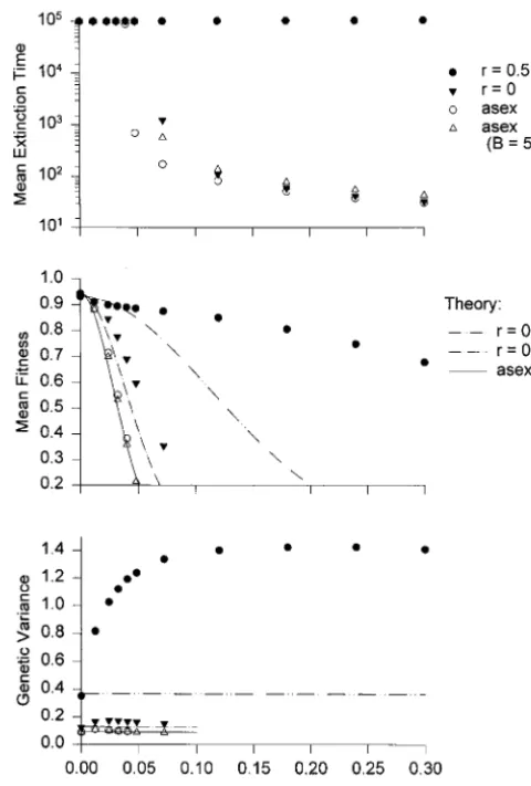
Figure 1 demonstrates the advantage that sex and recombination may confer to sexually reproducing pop-ulations in a directionally changing environment. As a function of the rate of environmental change, k, it
compares the mean extinction time, the mean fitness, Figure1.—Evolution and extinction of sexual and asexual populations under a directionally moving optimum. For all and the genetic variance for two sexually reproducing
data shown, the genomic mutation rate is U50.02, the input populations, one with and one without recombination,
of mutational variance is Vm50.001, and the mutation distri-and for two asexual populations, which differ by the bution is normal with mean zero and variancea250.05. The number of offspring produced. The data points are strength of stabilizing selection is Vs5 10, and the carrying capacity is K521152048. The top displays the mean time obtained from simulations, and the lines are from
the-to extinction as a function of the rate of environmental change ory as explained below. For all data shown, the carrying
k, the middle displays the mean fitness, and the bottom the
capacity is K 5 2115 2048. The number of offspring
average (additive) genetic variance. Solid circles, a freely re-produced per adult is B55 for the two sexual and one combining sexual population (n550 loci); solid triangles, a asexual population, and B5 50 for the other asexual nonrecombining sexual population; open circles, an asexual population with B5 5 as the two sexual populations; open population. This value is used to show that for a large
triangles, an asexual population with B550. The solid lines range of parameters, even a 10-fold advantage of asexual
in the middle and bottom are obtained from (14) and (10), reproduction would not counterweigh the advantage of respectively, the dash-dotted lines from (14) and (11), and sex in this kind of changing environment. the dash-double-dotted line from (14) and (12). Thus, mean Figure 1 (top) displays the mean time to extinction fitness is calculated by assuming that the variance remains
constant at its equilibrium value. for the four types of populations. For the whole range
of k values, a recombining sexual population persists indefinitely, i.e., for.105generations when simulations
if k $ 0.12. The situation is even worse for asexual were stopped. Additional simulations (not displayed)
populations with the same B. They go extinct within show that for k50.42 this population still persists for
,1000 generations if k$0.05. A 10 times larger B leads .105 generations, while for k5 0.48 and k5 0.72, its
to a longer persistence time for a small range of k values, mean extinction times are 24,000 and 17 generations,
but does not help for large k. As soon as k$0.12, which respectively. A nonrecombining segregating population
corresponds to 10% of a phenotypic standard deviation, can permanently withstand only a much lower rate of
asexual populations become extinct within,100 gener-environmental change. It goes extinct within some 1000
can easily persist through such a period of environmen-tal change. For the recombining and nonrecombining sexual, and for the asexual populations with B 5 50 and B5 5, approximate values for the critical rate of environmental change are kc50.69, 0.085, 0.080, and 0.050, respectively. They agree reasonably well with the simulation results.
Figure 1 (middle) displays the observed mean fitness together with theoretical approximations obtained from (14) by substituting the following values for the genetic variance: for the two asexual populations, the stochastic Fleming approximation (10) is used for all k. This pro-vides an accurate approximation for the observed mean fitness. For the two segregating populations and k.0, no good analytical approximations for the variance
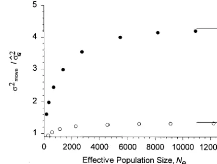
Figure 2.—Increase of genetic variance under a moving s2
moveare available. Substitution of the observed values optimum as a function of population size. The mutational of genetic variance into (14) yields precisely the ob- parameters are as in Figure 1. Solid symbols, a sexual, freely recombining population (Vs510, k50.04, and B52); open served mean fitness, thus supporting the Gaussian
the-symbols, an asexual population (Vs510, k50.012, and B5 ory (deviations are on the order of 0.1%; results not
5). The lowest population size is K 5 27 (N
e ≈ 170). For shown). To demonstrate the extent to which the
ob-populations,Ne≈150, rapid extinction occurs for the above served evolution of the genetic variance increases mean values of k. The lines on the right-hand side are for N
e5∞ fitness, the mean fitness of equivalent sexual popula- and are calculated as described in the text.
tions is plotted, but using the equilibrium genetic vari-ance (dash-dotted lines). The results demonstrate that
already in a slowly changing environment (k ≈ 0.05, lation to 50 loci by assuming global linkage equilibrium (LE).
which corresponds to a rate of environmental change
ofz5% of a phenotypic standard deviation per genera- Information about linkage disequilibrium was ob-tained by calculating the LE variance, i.e., the variance tion), the mean fitness of asexual populations is reduced
by almost a factor of five compared with an otherwise computed from the gene frequencies by assuming Hardy-Weinberg proportions and LE [Bulmer(1980) equivalent, but recombining, population. Thus,
compe-tition between such populations will almost certainly calls this the genic variance]. In all cases, the LE variance was larger than the additive genetic variance, thus indi-lead to the loss of the asexual population.
Figure 1 (bottom) shows that the genetic variance cating repulsion linkage disequilibrium. For freely re-combining populations and the data displayed in Figure increases substantially for a freely recombining
popula-tion (up to approximately fourfold), while for an asex- 1, the average LE variance was at most 13% higher than the additive genetic variance, with a much smaller ual diploid population the variance is nearly
indepen-dent of k (the maximum increase being 20%), and for increase for a resting or very slowly moving optimum. For the nonrecombining sexual populations as well as the segregating but nonrecombining population the
maximum increase isz40%. The variance of the asexual the asexuals, the LE variance was higher by up to a factor of 17.5 (in both cases), and this occurred for a population with B550 is almost identical (smaller by
z3%) to that of the population with B55, because its resting optimum. With a moving optimum, this factor decreased to values between 2 and 3 as k approached its effective size is smaller byz10%. For k50, all observed
variances are very close to their analytical approxima- maximum sustainable rate. In nonrecombining sexuals and asexuals, the amount of linkage disequilibrium in-tions with relative errors,5%.
The amount by which the genetic variance increases creased rapidly as population size and strength of stabi-lizing selection increased (data not shown).
relative to its equilibrium value depends on population
size. Because of the stabilizing component of selection, Additional simulations were performed for extremely weak (Vs 5 100) and very strong (Vs 5 5) stabilizing the variance must remain bounded even in an infinite
population. However, it is not clear how large a popula- selection. Under weak selection, recombining popula-tions responded with a much smaller increase of genetic tion has to be to approach this upper limit. For a sexual
and an asexual population, Figure 2 displays the ratio variance (s2
move/sˆ2G51.26 for k5 0.04 and Ne 5 2276 compared withs2
move/sˆ2G5 3.54 for Vs510), while under of the stationary variance under a moving optimum to
that under a resting optimum as a function of effective strong selection, the increase was even larger (s2 move/ sˆ2
G54.70, all other parameters unchanged). By
con-population size. The lines on the right-hand side are
for Ne5∞. Their values were determined by numerical trast, asexual populations had their variance reduced under weak stabilizing selection (s2
move/sˆ2G5 0.62 for
iteration of the deterministic one-locus
that an increase would enhance mean fitness. Under of Charlesworth but derives an approximation that is accurate for a wide range of parameters. It assumes a very strong selection and all other parameters
un-changed, the variance of asexual populations also in- Gaussian distribution of phenotypic values. The starting point is Equation 6a, which allows representation of the creased (s2
move/sˆ2G 5 1.49). Because of their much
greater genetic variance, the fitness advantage of sexual mean phenotype in generation t, Gt, as a sum of sines, parallel to Equation 28 ofCharlesworth(1993b). The populations over asexuals even increased with weaker
selection (data not shown). Given our knowledge about resulting expression can be approximated by an integral that produces
strength of stabilizing selection, values of Vsare more likely to be.10 instead of lower (Turelli1984;Endler
1986). Gt5
AstL
s2
tL21 4p2
[2pest(12t)22pcos(2p(t2 1)/L)
To explore the role of the mutation rate, simulations
were performed with smaller mutation rates, i.e., with 2 s
tL sin(2p(t2 1)/L)], (16)
a genomic mutation rate of U50.002. With this
muta-where stis the selection intensity (4). Defining the lag
tion rate and all other parameters as in Figure 1, asexual
byDt 5 Gt2 ut and averaging over one period of the
populations responded to a moving optimum with an
cycle (after a sufficiently long initial phase has elapsed), increase in variance of up to 80% (compared with 24%
one arrives at the approximation for the expected in the case U50.02), while freely recombining sexual
squared lag populations experienced a maximum increase of
vari-ance by a factor of nine (compared with a factor of four
E[D2] ≈lim
m→∞
1
Le
mL1L mL D2tdt
if U50.02).
5A2[s2L2(12cos(2p/L))12sLpsin(2p/L)12p2]
s2L214p2 A PERIODICALLY CHANGING OPTIMUM
While the moving-optimum model may be applicable
≈2A2p2(11s)2
s2L214p2 , (17)
to sustained, long-term environmental changes, such as climatic trends, many species are subject to changes on a much shorter time scale. This is particularly true for
where s is the asymptotic value of stThe latter
approxi-species with short generation times. A frequently
en-mation in (17) requires (2p/L)2 ! 1. Substitution of countered scenario may be that of a periodically varying
(17) into log Wt, as calculated from (7a), produces an
environment. We investigate population persistence,
accurate approximation for the expected log-mean fit-adaptive evolution, and the role of genetic variance in
ness. such an environment and compare recombining sexual
An approximation for the average mean fitness, populations with nonrecombining sexuals and diploid
Wper, can be obtained from (17) and (7a) by a straightfor-asexuals.
ward Taylor approximation. Defining For the Gaussian phenotypic model,Charlesworth
(1993b) andLandeandShannon(1996) derived
con-l 51 2E[D
2]/(V
s1 s2G)≈
A2p2
Vs(s2L21 4p2) , ditions under which an increase of genetic variance
leads to an increase of mean fitness if the fitness
opti-we get mum changes periodically. Charlesworth assumed
dis-crete generations, while Lande and Shannon assumed
Wper≈W
l
exp[2l 11 4l
221 6l
3], (18) continuous time. These conditions are more stringent
than with a linearly moving optimum because, in
partic-where Wlis the equilibrium mean fitness as given by ular with short-period fluctuations, tracking the
opti-(13). For most purposes, the term involvingl3can be mum is hardly possible and a low genetic variance is
omitted in (18). The quantity l agrees with the load favorable. As already mentioned above, there are cases
component derived byLandeandShannon(1996) for where the genetic system prevents an increase of genetic
a continuous-time model for cyclical change. variance, or even leads to a decrease, although a higher
From (18), sufficient (approximate) conditions can variance would increase mean fitness. Therefore,
com-be derived ensuring that an increase in genetic variance puter simulations seem to be inevitable to obtain
reli-causes an increase in mean fitness. These are able results for this complex model. In addition, we
need an extension of the above-mentioned theory
be-A2.V
s and 0, 9p 2
L229p2, s 2
G
Vs
,0.15. (19) cause, even after correcting for a misprint,
Charles-worth’s formula (30) for the expected log-mean fitness
is accurate only for short periods L and extremely small Figure 3 displays the mean fitness as function of the genetic variance for five different periods, L, and (top s2
G/Vs. Otherwise, it underestimates the true value
Figure 3.—Dependence of mean fitness on the genetic variance in a periodically changing environment. The popula-tion size is infinite and the strength of stabilizing selecpopula-tion is
Vs510, i.e.,v 53. The curves are calculated from (18). They are very close to exact values, as obtained from numerical integration of (7a) using (16).
change by major jumps, genetic variance is detrimental to mean fitness, while for medium or long periods, more
Figure4.—Evolution and extinction of sexual and asexual genetic variance is beneficial unless the variance is ex- populations in a periodically changing environment. The mu-tremely large. This is similar toLandeandShannon’s tational parameters are as in Figure 1, the strength of stabiliz-(1996) results but in partial contrast toCharlesworth ing selection is Vs510 (v 53), and the carrying capacity is K521152048. The amplitude (maximum displacement of (1993b), who underestimated the advantage of
in-the optimum) is A52v 56. The top displays the mean time creased genetic variance. Obviously, in a periodically
to extinction as function of k54A/L, which can be interpreted changing environment, an increase of genetic variance as the average rate of environmental change during one pe-leads to an increase of mean fitness only under more riod of length L. The length of the period (in generations) restrictive conditions than in a directionally changing is indicated on the top. The middle displays the mean fitness, and the bottom, the average (additive) genetic variance. Solid environment. This does not imply, however, that the
circles, a freely recombining sexual population (n550 loci); genetic variance actually does increase under such
con-solid triangles, a nonrecombining sexual population; open ditions. circles, an asexual population. The solid lines in the middle The detailed evolution of finite sexual and asexual and bottom are obtained from (18) and (10), respectively, the dashed lines from (18) and (11), and the dash-double-populations in a periodically changing environment was
dotted line from (18) and (12). For all lines, mean fitness is investigated by Monte Carlo simulations as described
calculated by assuming that the variance remains constant at above. No assumptions are imposed on the distribution
its initial equilibrium value (k50). of phenotypic (or genotypic) values. Some of the results
are summarized in Figures 4 and 5. The quantities of
interest are displayed as functions of k54A/L, which is chosen to be 2v, which implies that, at the most can be interpreted as the rate of change of the optimum extreme position of the optimum (A units from the averaged about one full cycle (during which the opti- origin), the originally optimal phenotype (at position mum moves 4A units, measured in multiples of s2
E). 0) has a fitness of 13.5%. The top shows that in this
In this case, it makes sense for a population to stay where it is and wait until the environmental optimum returns. Clearly, this requires that the population is able to maintain a minimum viable population size during the period of low fitness.
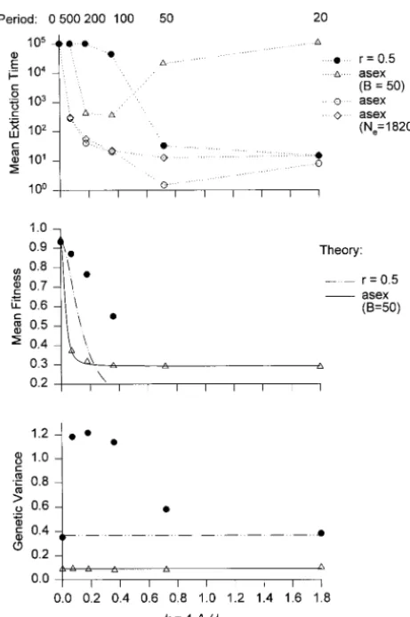
Figure 5 is similar to Figure 4, but with a higher amplitude of environmental fluctuations (A 5 3v). Then the fitness of the originally optimal phenotype is only 1.1% if the environmental optimum is at its most extreme position, A. The figure compares a freely re-combining sexual population with three different dip-loid asexuals: one with all other parameters equal, a second that produces 10 times as many offspring (B5 50), and a third whose carrying capacity is 8 times higher (K 5214, N
e518,205). Again, for long periods L, i.e., slow environmental change, the sexual population has the highest mean extinction time and mean fitness. For a rapidly changing optimum, however, it is the asexual population that produces B550 offspring that has the longest persistence time, although it has a much lower genetic variance than the sexual population (bottom). The lines (middle) display the mean fitness as expected with a constant genetic variance. This figure clearly dem-onstrates that in a rapidly changing, periodic environ-ment, it is not the flexibility of the genome and the resulting better adaptability that improves population persistence. Instead, other strategies, such as produc-tion of more offspring, may be more successful. For a slowly changing optimum, good adaptation is the best response to environmental change.
Figure5.—Evolution and extinction of sexual and asexual
Further simulations (results not shown) have been populations in a periodically changing environment. This is
similar to Figure 4, but with a larger amplitude of environmen- performed with smaller population sizes and lower am-tal fluctuations (A53v 59). Solid circles, a freely recombin- plitudes (A5 v). Although for lower population sizes ing sexual population (n550 loci); open circles, an equivalent the increase of variance in freely recombining popula-asexual; open triangles, an asexual with B 5 50; open
dia-tions is generally much lower, they still persist longer monds, an asexual population with B55 and K5214(effective
and have a higher mean fitness than otherwise equiva-size Ne518,205). The solid lines in the middle and bottom
are obtained from (18) and (10), respectively, and the dash- lent but nonrecombining sexual or asexual populations. double-dotted line from (18) and (12). For all lines, mean Again, the advantage of sex and recombination is most fitness is calculated by assuming that the variance remains pronounced for large amplitudes A and long periods L. constant at its initial equilibrium value (k50).
If mutational effects are drawn from a reflected gamma distribution instead of a Gaussian (cf. Keight-leyandHill1988;Bu¨ rgerandLande1994), qualita-The middle shows that the freely recombining
popula-tion has a much higher mean fitness than the two other tively similar results are obtained. For large recombining populations (K5211, N
e52276) and medium or long populations if the length of the period is between 100
and 500. The lines in the middle represent the mean periods, L, a slightly higher increase of variance occurs in comparison with otherwise equivalent populations. fitness that would be obtained if the variance did not
increase under the periodic optimum. This yields good This yields a slightly increased mean fitness. For small recombining populations (K 5 28, N
e 5 285), such a approximations for the nonrecombining and the
asex-ual population, but not for the recombining population, distribution also led to a higher average genetic variance and mean fitness, but to lower mean extinction times. because its genetic variance increases substantially
un-less the period, L, is very short (L#20). This is shown Actually, mean extinction times have a much higher variance in this case compared with that of a Gaussian in the bottom. Thus, for this kind of environmental
change, recombination improves mean fitness and in- mutation distribution, because only a few populations are picking up rare mutants with large positive effects creases population persistence only if the period of the
cycle is long, i.e., evolution is slow. This advantage of on fitness, while others go extinct rapidly. Thus, with a highly kurtotic mutation distribution the dynamics seem recombination is due to the fact that it enables
popula-tions to increase in genetic variance. If the optimum to be driven to a greater extent by single, large muta-tional events.
Finally, it is worth mentioning that if the observed an explicit genetic multilocus model and by assuming finite population size and population regulation. Ge-genetic variance is substituted into Equation 18, a very
accurate approximation of the observed mean fitness is netic variation is assumed to be maintained by mutation-selection balance. In a constant environment that exerts obtained, thus supporting the mathematical theory.
stabilizing selection on the trait under consideration, sexually reproducing populations have more genetic A RANDOMLY FLUCTUATING OPTIMUM
variance than mutationally and demographically equiva-lent asexual populations. This leads to a slightly higher The Gaussian theory ofCharlesworth(1993b)
pre-dicts that for an optimum that fluctuates randomly ac- equilibrium load of sexual populations. If, however, ad-aptation becomes necessary due to environmental cording to white noise with mean zero, variance Vu, and
no autocorrelation, an increase of genetic variance leads change, then sexual populations can respond faster and gain a substantial selective advantage over asexuals. to an increase of mean fitness only if Vu.2Vs. A similar
result was obtained bySlatkinandLande(1976), while In accordance with results of Charlesworth (1993a,b), this study demonstrated an advantage of re-LandeandShannon(1996) showed that in a
continu-ous-time model more genetic variance always increases combination and sexual reproduction over asexual re-production under sustained directional change of the the load.
Monte Carlo simulations with the model described environment as well as under a slowly periodically changing environment with a large amplitude. This ad-above have shown that in both asexual and sexual
popu-lations the genetic variance remains virtually constant vantage was measured both in terms of mean persistence times as well as mean fitness. However, under the pres-if Vu# Vs, in accordance with similar results ofLande
(1977) andTurelli(1988). Hence, fluctuating selec- ent genetic model, in which mutations at each locus are drawn from a continuous distribution and the num-tion with a constant average optimum and no
autocorre-lation is not a mechanism to increase genetic variation ber of loci is large but finite, sufficiently large sexually reproducing populations with high levels of recombina-(Turelli1988).
In contradistinction to theory (Slatkin andLande tion respond to environmental change of the above-mentioned kind by a substantial increase of (additive) 1976; Charlesworth 1993b; Lande and Shannon
1996), for fluctuations with variance Vu5Vs510, sexual genetic variance, while nonrecombining sexual or asex-ual populations do not, or do to a much lesser extent. freely recombining and asexual populations of effective
size Ne 5 1140 and with B 5 5 went extinct after an This flexibility of the genome confers a significant addi-tional advantage to recombination (and sexual repro-average of z7900 and 6600 generations, respectively
(100 replicated runs). Asexual populations with twice duction) that goes far beyond the evolutionary advan-tage recognized by Charlesworth (1993b) on the the mutation rate and intermediate variance had a mean
extinction time of 6900 generations. The mean fitnesses basis of the Gaussian phenotypic model that assumes that genetic variance does not change under selection. averaged over the persistence time, however, were
ranked inversely to the genetic variances, but the differ- In a constant environment, in a randomly fluctuating environment with small variance and no autocorrela-ences were not significant. More genetic variance is
ben-eficial in this case, probably because under rare large tion, and in a rapidly changing periodic environment with short periods, asexually reproducing populations excursions of the optimum more individuals survive in
populations with a broader distribution. Hence, the the- have a higher mean fitness and a longer persistence time than freely recombining sexual populations. This ory based on the assumption of a Gaussian phenotypic
distribution predicts an advantage for lower genetic vari- is in qualitative agreement with the Gaussian theory (Slatkin and Lande 1976; Charlesworth 1993b; ability and asexual reproduction when there is none. If,
however, asexuals have twice the growth rate of sexuals, Lande and Shannon 1996). In such “unpredictable” environments, a higher reproductive rate is a more suc-then their mean persistence time is approximately
tri-pled and, thus, higher than that of the corresponding cessful strategy for survival than elevated levels of ge-netic variance. In contrast to theoretical predictions, sexual population.
For smaller Vu, asexual populations have a slightly however, more genetic variation and, hence, sexual re-production can be beneficial in a randomly fluctuating higher mean fitness than sexuals because of their lower
genetic variance (results not shown). Indeed, mono- environment if the standard deviation of the fluctua-tions exceeds the width of the fitness function. Nonre-morphic populations have the highest fitness and
ex-tinction time under such a model (cf. Bu¨ rger and combining sexual populations (so that there is only segregation between chromosomes) are always in be-Lynch1995).
tween these two extreme cases but much closer to the asexuals. It is also of interest to note that in a randomly DISCUSSION
fluctuating environment an increase of environmental variance may be beneficial (Bull1987).
This investigation departs from previous work on the
mean phenotype and mean fitness is accurate for direc- function. If the per-locus mutation rate is low (20mVs, a2), then the equilibrium distribution is highly kurtotic, tional and periodic environmental change, provided
the genetic variance is known. A satisfactory theory for so that a large fraction of genetic variance is maintained by rare alleles with large effects and the equilibrium the genetic variance, however, exists only for a constant
environment (mutation-stabilizing selection-drift bal- variance is closely approximated by the HC approxima-tion. Under these conditions, the equilibrium genetic ance). In this case, accurate approximations for
recom-bining and nonrecomrecom-bining sexual populations, as well variance is much lower than the Gaussian orFleming’s (1979) approximation; cf. Bu¨ rger and Hofbauer as for asexuals, have been developed. Because for a
range of realistic parameters, the genetic variance of (1994). It has already been shown that for various forms of directional selection such a population responds with nonrecombining sexual and of asexual populations
re-mains fairly constant, their evolution can be reasonably a huge increase of variance, which is mainly caused by sweeps of rare alleles with large effects (Bartonand well predicted. For recombining sexual populations this
is not true. Below, we discuss why this is so. Turelli1987;Bu¨ rger1993). Under the moving-opti-mum model, a population also responds with an in-KondrashovandYampolsky(1996a,b) reported an
increase of genetic variance in models of periodic envi- crease in variance and, finally, the frequency distribu-tion settles down to a traveling wave that lags behind ronmental change, but found that genetic variance
in-creased by up to three orders of magnitude. Below, we the optimum by an amountD 5(kVs11⁄2c3)/c2and has variance
discuss the reason for this large increase and why such a large increase seems to be unrealistic.
c25
√
mVsa21 D· c3 21⁄2c4, (20)Evolution of genetic variance:The simulation results
reported in this article lead to the following questions: where c
3 and c4 are the third and fourth cumulant of Why is the increase of genetic variance in response to the haploid allelic distribution (see appendix; for a directional environmental change much more pro- normal distribution c
35 c4 5 0). Unless the optimum nounced in sexually reproducing populations than in moves extremely slowly, directional selection induces a asexuals? Why did Kondrashov and Yampolsky lag and a skewness such thatD· c
3.1⁄2c4. (Iterations of (1996a) detect increases of variance that are so much the deterministic equations show that this is true ifm, higher than the present ones? More generally, we may V
s, and k are each varied over two orders of magnitude ask what are the prerequisites on the genetic system around the typical parameters considered in this arti-and the mode of selection that allow evolution of the cle.) Thus, the asymptotic variance under the moving genetic variance? optimum is higher than the Gaussian predictionsˆ2(G). Explanations for the distinct evolutionary behavior of This explains the increase of variance at a single locus recombining populations can be given on two levels of with a low mutation rate. For a freely recombining popu-sophistication: first, on an intuitive, qualitative level, and lation, little linkage disequilibrium builds up (as sub-second, on a quantitative, formal one. If a new favorable stantiated by the computer simulations) and the total mutant in a freely recombining population is not lost genetic variance is simply the sum of the haploid single-by random drift, it will eventually be recombined with locus variances.
genotypes of high fitness and can sweep rapidly through These considerations not only explain the increase the population, thus leading to a temporary increase of of variance observed for large recombining populations genetic variation. With a constant supply of new muta- but also provide a rule of thumb for its magnitude. tions and directional selection (as caused by a gradually The factor by which the genetic variance increases is and predictably changing environment), this leads to bounded below bys
ˆ2(G)/sˆ2(HC), so that an increased level of additive variation. The larger the
population size, the larger the increase will be (see Fig- s2 move sˆ2
G
$ a 2
√
mVs, (21)
ure 2). If a new favorable mutant occurs in a nonrecom-bining or asexual population, it will forever remain tied
unless the rate of environmental change, k, is very close to its genome and all the disadvantageous mutants. This
to zero. line may increase in frequency if its fitness is high
In finite populations, genetic variance is eroded by enough, but the increase may be slow and weak. In
random drift at a rate proportional to 1/Neper genera-particular, the line will never go to fixation unless the
tion. In particular, in small populations (Nea few hun-genomic mutation rate is extremely low.
dred or less), rare alleles of large effect occur much less A quantitative understanding of the evolution of
ge-frequently than in large populations and are more likely netic variance can be obtained from
mutation-selection-to be lost by drift. Because these are responsible for balance theory and the equations for the rate of change
most increase of variance, this increase is smaller or of the mean and variance at a haploid locus (appendix).
absent in such populations (cf. Figure 2; but alsoBu¨ rger Let us first consider an effectively infinite population
1993; Bu¨ rger and Lynch 1995). A lower bound can and a single haploid locus that, initially, is in
Gaussian approximation through the SHC approxima- KondrashovandYampolsky(1996a,b) investigated tion, i.e., a quantitative trait in a periodically changing environ-ment that is determined by equivalent diallelic loci with equal forward and back mutation rates [Barton’s s2
move sˆ2
G
$ a 2
√
mVsNe1 Vs/a2
Ne11⁄2
√
Vs/(ma2). (22)
(1986) model]. They reported increases of variance in amphimictic populations of two and three orders of The right-hand side approaches one as Nebecomes small.
magnitude and somewhat lower increases in apomictic Comparison with the simulation results shows that (21)
populations. On the basis of the above theory this can and (22) produce fairly good approximations as long as
be explained by their parameter choice. Their typical the HC approximation is much lower than the Gaussian,
parameter set consists of 36 loci with a mutation rate
i.e., ifmVsis sufficiently small relative toa2.
of 1025, yielding a gametic mutation rate of,1023, and The above approximations explain why a lower
muta-very strong stabilizing selection (in our notation, Vs/a2≈ tion rate and stronger stabilizing selection entail a
1.5). Thus, their equilibrium populations maintain al-higher increase of genetic variance: under such
condi-most no genetic variance under mutation-selection bal-tions the ratio of the Gaussian and the HC
approxima-ance. For this parameter set, (21) predicts a.100-fold tion is larger.
increase of genetic variance, which is in qualitative By contrast, if the per-locus mutation rate is high
agreement with their simulation results. The problem, (9mVs. a2), then in an infinite population the
equilib-however, is that reviews of data suggest that gametic rium distribution at a haploid locus is very close to
mutation rates are much larger (on the order of 1022) normal and its variance is close to the Gaussian or
Flem-and stabilizing selection is often weaker (cf. Turelli ing’s prediction. As discussed in the section on
muta-1984). The result, that in a periodically changing envi-tion-selection-drift balance, this situation applies to
ronment the advantage of sex and recombination is asexual and nonrecombining sexual populations.
most pronounced for large amplitudes and intermedi-Hence, their increase of genetic variance is very small.
ate or long periods, however, is in qualitative agreement Under weak stabilizing selection, the variance can even
withKondrashovandYampolsky(1996b). decrease (as mentioned above) because, then, the
as-The model employed in this article can be extended ymptotic distribution becomes negatively skewed and
to include a modifier for the recombination rate. It the lag very large.
would be interesting to investigate if this led to a higher The distribution of genotypic values remained close
to Gaussian for all investigated cases, and this is in accor- selective advantage of the modifier than in Charles-dance with previous results (Bu¨ rger1993;Turelliand worth’s (1993b) investigation with a constant variance. Barton1994;Bu¨ rgerandLynch1995). More surpris- Other strategies for survival in a changing
environ-ingly, however, even at a haploid locus the asymptotic ment:On the basis of (15) for the maximum sustainable distribution is close to Gaussian for any choice of param- rate of environmental change, it can be estimated how eter values as long as the directional-selection compo- much larger the intrinsic growth rate of a population nent is stronger than mutation. Noticeable departures must be to offset an increase of genetic variance. A occur only if k! ma2 (results not shown). The reason
simple calculation reveals that a rough condition is the can be seen from the cumulant equations in theappen- following:
dix: without mutation, a Gaussian distribution remains
Gaussian if selection occurs according to the moving ln B2 ln B1
.
1
s21 s2 22
2 . optimum model and, apparently, is stable. Deviations,
through increased kurtosis (c4.0), are brought about
Thus, the advantage of a doubling of the genetic vari-only by mutation.
ance can be achieved only by an approximate quadru-In a periodically changing environment, an increase
pling of the intrinsic growth rate, ln B. Equivalently, a in variance occurs that is quantitatively similar to that
twofold cost of sex (B252B1) will be offset by an increase in a directionally changing environment, if the
ampli-of variance byz20%. It is also obvious from (14) and tude is large (A . 2v) and the period is long (L $
(15) that an increase of population size has only a negli-100), so that directional selection dominates (cf. Figures
gible influence on the critical rate of change (as well 1, 4, and 5). Otherwise, even in freely recombining
as on the expected mean fitness and the expected mean populations no or very little increase occurs. This is in
extinction time), unless it leads to an increase of genetic qualitative accordance with the Gaussian theory, which
variance. It may be of conservation biological concern shows that under such environmental change a higher
that in recombining species, a noticeable increase of variance does not enhance mean fitness. However,
usu-variance under directional selection will only occur if ally the genetic variance does not evolve to the level at
the effective population size is.200–300. In a periodi-which, according to the Gaussian theory, mean fitness
cally changing environment, a higher growth rate may would be maximized. This, obviously, is a consequence
substantially enhance population persistence. of the constraints set up by the genetic system and the