Balancing Selection at Closely Linked, Overdominant Loci in a Finite Population

Copyright2000 by the Genetics Society of America

Balancing Selection at Closely Linked, Overdominant Loci

in a Finite Population

Montgomery Slatkin

Department of Integrative Biology, University of California, Berkeley, California 94720-3140

Manuscript received July 23, 1999 Accepted for publication November 19, 1999

ABSTRACT

High levels of allelic diversity and strong linkage disequilibrium are found in the major histocompatibility (MHC) system in humans and other vertebrates. This article proposes several descriptive statistics that quantify the extent and pattern of strong linkage disequilibrium between pairs of highly polymorphic loci. It also develops an approximate analytic theory incorporating the effects of balancing selection, mutation, recombination, and genetic drift at two closely linked loci and compares the theoretical predic-tions with published surveys of the MHC class II loci, DQA1 and DQB1, in humans and nonhuman primates. The descriptive statistics proposed include the fraction of complementary haplotypes (haplotypes with D⬘ ⫽1), the fraction of excess haplotypes, and the numbers of alleles at each locus in complementary haplotypes with one or more alleles at the other locus. The model assumes the infinite alleles model of mutation and the symmetric overdominance model of selection. Analytic approximations in some cases are obtained in the strong selection, weak mutation (SSWM) limit introduced by J. Gillespie. The predictions of the approximate analysis are confirmed by simulation. Both the analytic theory and simulations show that relatively few haplotypes will be found when selection is strong and recombination is weak relative to genetic drift. The model can reproduce many of the observed patterns at DQA1 and DQB1 provided that the recombination rate is assumed to be very small.

B

ALANCING selection resulting from either over- nant loci, each of which has a potentially large number of alleles. The theory predicts the numbers of alleles dominance in fitness or genetic self-incompatibility

maintains many more alleles at a locus than would be maintained at each locus and the pattern of allelic asso-ciation in haplotypes. The theory is based on Gilles-expected at a neutral locus with the same mutation rate.

Several theoretical studies provide approximations that pie’s (1984) strong-selection, weak-mutation (SSWM) approximation, which has been shown to be useful for allow prediction of the number of alleles maintained

by strong balancing selection in finite populations modeling balancing selection, mutation, and genetic drift at a single locus (Sasaki1989, 1992;Slatkinand (KimuraandCrow1964;Takahata1990;Sasaki1992;

VekemansandSlatkin1994;SlatkinandMuirhead Muirhead 1999).

Linkage disequilibrium in MHC:The present

theoreti-1999). Balancing selection affecting two closely linked

cal study was motivated in part by observations of linkage loci can maintain substantial allelic diversity at each

disequilibrium in the major histocompatibility (MHC) locus and also maintain strong linkage disequilibrium

region in humans and other vertebrates. The MHC re-between them, but the problem is much harder to

ana-gion contains numerous loci that are closely linked lyze. There are many theoretical studies of linkage and

and highly polymorphic. Particularly good evidence of selection affecting diallelic loci in infinite populations

strong linkage disequilibrium is found in the class II (Lewontin and Kojima 1960; Karlin and Feldman

loci, DQA1 and DQB1, in humans and some other pri-1970) and a few studies of linkage and selection when

mates. In humans, these two loci areⵑ20 kb apart on the one of the loci has more than two alleles (Christiansen

short arm of chromosome 6. Although no recombinants and Feldman 1975; Feldman et al. 1975). There are

between them have been reported, the recombination also several studies of linkage and mutation in finite

rate can be estimated roughly to be 0.0002 if 1 Mb is populations (Hill and Robertson 1968; Griffiths

assumed to correspond to a rate of 0.01 (1 cM). Recom-1981). But there are no analytic studies that model the

bination rate is known to vary with location in the MHC combined effects of selection, mutation, and linkage in

region in humans (Cullenet al. 1997), so the

recombi-finite populations. In this article, I develop an

approxi-nation rate between DQA1 and DQB1 might well be mate analytic theory for two closely linked

overdomi-⬍0.0002.

At DQA1, 16 alleles are known, 8 of which are in appreciable frequency worldwide; at DQB1, 25 alleles

Address for correspondence: Montgomery Slatkin, Department of

Integ-are known, 15 of which Integ-are in appreciable frequency

rative Biology, University of California, 3060 Valley Life Sciences Bldg.,

Berkeley, CA 94720-3140. E-mail: [email protected] worldwide (Marsh 1998). The two loci code for

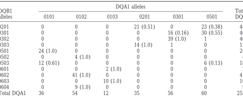
TABLE 1

DQA1-DQB1 haplotype numbers andDⴕvalues in CEPH families

DQA1 alleles

DQB1 Total

alleles 0101 0102 0103 0201 0301 0501 DQB1

0201 0 0 0 21 (0.51) 0 23 (0.38) 44

0301 0 0 0 0 16 (0.16) 30 (0.55) 46

0302 0 0 0 0 39 (1.0) 1 40

0303 0 0 0 14 (1.0) 1 0 15

0501 24 (1.0) 0 0 0 0 0 24

0502 0 4 (1.0) 0 0 0 0 4

0503 12 (0.61) 0 0 0 0 6 (0.13) 18

0601 0 0 2 (1.0) 0 0 0 2

0602 0 41 (1.0) 0 0 0 0 41

0603 0 0 10 (1.0) 0 0 0 10

0604 0 9 (1.0) 0 0 0 0 9

Total DQA1 36 54 12 35 56 60 253

The table shows haplotype numbers and D⬘values for 253 independent chromosomes from Centre d’Etude du Polymorphism Humain (CEPH) families (Begovichet al. 1992, Table III). The D⬘values were computed after the two haplotypes found only in a single copy (0501-0302) and (0301-0303) were deleted. There are two multi-A alleles (0102 with i⫽3 and 0103 with i⫽2). There is a significant excess (at the 1% level, based on a␹2_{test) of all haplotypes found in more than one copy, except for 0501-0503.}

peptides, DQ␣ and DQ␤, that form a heterodimer. als bred in captivity, so some of the chromosomes sam-pled were possibly identical by descent because of past

Kwok et al. (1993) showed that alleles at each locus

could be grouped and that haplotypes formed from inbreeding. The nonindependence of chromosomes would affect the formal statistical analysis of the data. alleles in incompatible groups did not produce stable

cell surface heterodimers. These “prohibited” haplo- In this article, the data are compared only qualitatively to theoretical predictions. They are used to illustrate types had not been present in population surveys (

Fer-nandez-Vin˜ a et al. 1991), but recently Grahovac et the application of the theory rather than to draw strong conclusions about the operation of selection in the

dif-al. (1998) found several of the supposedly prohibited

haplotypes in their study of Siberian populations. ferent species discussed. Although larger samples would be desirable, they are not currently available.

In humans, relatively few haplotypes are present and there is significant excess of almost all of them. Linkage disequilibrium is not complete and some alleles at

LINKAGE DISEQUILIBRIUM AT DQA1 are in strong disequilibrium with two or more

MULTIALLELIC LOCI alleles at DQB1 (Begovichet al. 1992). Some typical

data are presented in Table 1 and will be discussed in If there are only two alleles at each of two loci, the coefficient of linkage disequilibrium, D, defined by more detail later. DQA1 and DQB1 in chimpanzees

and gorillas show no significant linkage disequilibrium LewontinandKojima(1960), is sufficient to describe the degree of nonrandom association between those (GyllenstenandErlich1993). In the rhesus monkey

(Macaca mulata) DQA1 and DQB1 are in very strong loci. All other measures of nonrandom association can be expressed as functions of D and the two allele fre-linkage disequilibrium, and the pattern is different from

that found in humans (Sauermann1998). In a sample quencies. With more than two alleles per locus, no single measure of linkage disequilibrium provides a complete of 134 individuals, Sauermann(1998, Table 4) found

14 different haplotypes present in more than one copy. description; what measure or measures are best depends on the pattern in the data and the purpose of the analy-Each of the 14 haplotypes contained alleles at both

loci that were in no other haplotypes in the sample. sis. If the goal is to detect nonrandom association and to test its significance, then a measure based on the␹2 Sauermann (1998) attributed the difference between

the patterns in rhesus monkeys and in humans to statistic, as proposed byFeldmanet al. (1975) and

oth-ers, or the probability value from Fisher’s exact test, stronger selection acting on these two loci in the rhesus

monkey. used byPeterson et al. (1995), will serve. If, instead,

the goal is to focus on a particular allele at one locus All of these studies are based on samples of individuals

collected for other purposes, so the data cannot be and characterize the extent of disequilibrium with mark-ers at another locus, then the ␦ statistic, suggested by regarded as representing random samples from

individu-TABLE 2

disequilibrium involving most or all alleles at both loci

and there is no reason to focus on any particular allele _{State space and notation for the model with complete} at either locus. As in the data presented in Table 1, _{linkage: haplotypes found in a hypothetical data set with} very few of the many possible haplotypes are found 13 alleles at the A locus and 11 alleles at the B locus

and almost every haplotype shows significant excess or

A1B1, A1B2, A1B3(i⫽3) deficiency. Furthermore, many or most of the values of

A2B4, A2B5(i⫽2) Lewontin’s D⬘(1964) statistic (defined to be the ratio

A3B6, A4B7, A5B8(K⫽3) of the coefficient of linkage disequilibrium to its

maxi-A6B9, A7B9, A8B9, A10B9( j⫽4) mum possible value) for haplotypes present in more _A

11B10, A12B10( j⫽2) than one copy are 1 or nearly 1. Very strong linkage A13B11, A14B11( j⫽2) disequilibrium of this kind can be generated by strong

overdominant selection affecting both loci, as shown in In this case, I⫽2, J⫽3, K⫽3. At the symmetric, deterministic equilibrium described in the text, the frequencies of gametes the next several sections. To compare theory and data,

in each row containing more than one are equal. The fre-some descriptive statistics are necessary to quantify this

quency of those in the first row would be x3, those in the

pattern. _{second row would be x}

2, those in the third row would be z,

Fraction of complementary haplotypes: I adapt the _{those in the fourth row would be y}

4, those in the fifth and terminology of Feldman et al. (1975) and call haplo- sixth rows would be y2, andφ2⫽φ3⫽1⁄2,␳2⫽2⁄3, and␳4⫽1⁄3. types, which are present in more than a specified

num-ber of copies and for which D⬘ ⫽1, complementary

haplo-ing that one allele at B is associated with multiple alleles types. Allowing for a threshold is necessary because

at A. The number of multi-B haplotypes will be denoted haplotypes found in only one or a few copies may be

by J, and the fraction that are class j will be denoted by artifacts or aberrant for some reason. For the data in

␳j. An example of the use of this notation is given in Table 1, I use a threshold value of two copies, which

Table 2. means that two haplotypes, 0501-0302 and 0301-0303,

In Table 1, J ⫽ K ⫽ 0, I ⫽ 2, and φ2 ⫽ φ3 ⫽ 0.5. are ignored. One descriptive statistic is the fraction of

The allele 0102 at DQA1 is found in complementary haplotypes that are complementary. For the data in

haplotypes with three different alleles at DQB1, and Table 1, there are 14 haplotypes found in more than

0103 at DQA1 is found in complementary haplotypes one copy, and 8 of them have D⬘ ⫽1, so that fraction,

with two different alleles at DQB1. Note 0101, 0201, which is denoted by CF (for complementary fraction),

and 0301 at DQA1 do not contribute to I because the is 0.571.

0101-0503, 0201-0201, and 0301-0301 haplotypes are not

Fraction of extra haplotypes:Another descriptive

sta-complementary. InSauermann’s (1998) study of rhesus tistic is the number of haplotypes relative to the total

monkeys, I⫽ J⫽0, and K⫽ 14. possible number. The minimum possible number of

haplotypes is the larger of kAand kB, and is 11 for the data in Table 1. The maximum number is kAkB, which

DETERMINISTIC THEORY OF SELECTION is 66 for the data in Table 1. An index describing the

proportion of haplotypes greater than the minimum, Before considering the effects of mutation and ge-netic drift, I review and extend slightly results from which I call the fraction extra (FE) haplotypes, is FE⫽

(kH⫺kM)/(kAkB⫺kM), where kHis the number of haplo- the deterministic theory of overdominant selection and recombination. The selection model in this article is types and kMis the larger of kA and kB. This fraction is

0 if the minimum number is found and 1 if all possible the symmetric overdominance model (Christiansen andFeldman1975;Feldmanet al. 1975), in which the

haplotypes are found. For the data in Table 1, FE⫽

0.05. relative fitness of doubly heterozygous individuals is 1, of

doubly homozygous individuals is 1⫺ ␣, of individuals

Multi-A, multi-B, and unique haplotypes: It is useful

to characterize the complementary haplotypes in which heterozygous only at the A locus is 1⫺ ␤, and of individu-als heterozygous only at the B locus is 1⫺ ␥. The recom-each allele is found. If an allele at A is in a

complemen-tary haplotype with only one allele at B, that haplotype bination rate between the loci is c.

Two alleles per locus:This model with only two alleles will be called a unique haplotype, and the number of

unique haplotypes will be denoted by K. If an allele at at each locus has been analyzed by several authors begin-ning with Lewontin and Kojima (1960). We restrict A is in complementary haplotypes with i alleles at B,

that will be defined as one class i multi-A haplotype, our attention to the range of parameter values that seems most appropriate for the MHC region and assume indicating that one allele at A is associated with multiple

alleles at B. The number of multi-A haplotypes will be ␣,␤, and␥ are all between 0 and 1 and further that ␣ ⬎ ␤,␥.

denoted by I, and the fraction of multi-A haplotypes

that are class i will be denoted byφi. If an allele at B is The quantityε⫽ ␤ ⫹ ␥ ⫺ ␣plays an important role in the deterministic theory. Ifε⬎0, which is sometimes in complementary haplotypes with j alleles at A, that

homozy-gotes are closer on average to the fitnesses of the double librium given by (1) to prove that it is locally stable for small values of c.

homozygotes than they are to the fitness of the double

heterozygote. Ifε⬍0, negative epistasis, the opposite is The Karlin-McGregor theory tells us that a thorough analysis of a deterministic model with c⫽0 provides a the case. At present, there is no basis in saying whether

loci in the MHC or other systems are better modeled by complete understanding of the behavior of a determin-istic model of selection with very small values of c. We will assuming positive or negative epistasis, but both existing

deterministic theory and the new theory developed later see that the Karlin-McGregor theory is a useful starting point for analyzing overdominant selection in finite for a finite population show that the sign ofεis

impor-tant. populations, but that new results are found when

ge-netic drift and mutation are included. LewontinandKojima(1960) showed that, ifε⬎4c,

there is an equilibrium at which alleles at both loci are in frequency 1/2 and at which D is nonzero. Karlin

SSWM APPROXIMATION and Feldman (1970) proved that this equilibrium is

locally stable under the restricted ranges of values of␣, _{We begin with the analysis of the case in which c⫽} ␤, and␥considered here. Ifεⱕ0, no equilibrium with _{0, for which an analytic approximation can be obtained,}

D⬆0 exists for any c⬎ 0. _{and then use simulations to determine the effects of}

More than two alleles per locus:Feldmanet al. (1975) _{small amounts of recombination. With c⫽0, the model}

and Christiansen and Feldman (1975) studied this _{reduces to a model of selection at one locus, for which} selection model when one locus has more than two _{many general results are known (Nagylaki1992).} alleles. These articles show that positive epistasis is neces- _{Deterministic equilibria: Initially, we consider only} sary for the existence of stable equilibria with nonzero _{those equilibria that are relevant when there is positive} values of D.ChristiansenandFeldman(1975, p. 195) _{epistasis (ε⬎0). With no recombination, a new allele} found that, in a model with two alleles at one locus and _{at one locus will remain linked to the allele at the other}

m alleles at the other, stability of the equilibrium with _{locus that was on the chromosome on which it first}

only the haplotypes A1B1, . . . , A1Bm/2. A2Bm/2⫹1, . . . , A2Bm _{appeared, and it cannot be joined by recombination to} (m even) is possible only if c⬍ε/(2m). The upper bound _{any other allele present when it appeared. Thus, if A}

1 on c decreases inversely with the number of alleles at _{appears on a chromosome initially carrying B}

1, and

the B locus. _{there are m⫺ 1 other alleles at the B locus, B2. . . B}

m, We can obtain a similar result for the generalization _{A1cannot later be on a chromosome carrying B2. . . B}

m. of the Lewontin and Kojima model to the case with _{Mutation at B can then create new haplotypes carrying}

K alleles at each locus. The symmetry of the problem _{the mutant. For example, A1B}

m⫹1 could be created by suggests that the frequencies of all coupling haplotypes, _{mutation from B1to B}

m⫹1.

A1B1, . . . , AKBK, are the same, z, and the frequencies of _{At a complementary equilibrium, all haplotypes are} all recombinant haplotypes (AlBm for l ⬆ m) are the _{either multi-A haplotypes, multi-B haplotypes, or unique} same. There is always an equilibrium at which there is _{haplotypes. As before, I is the number of A alleles in} complete linkage equilibrium, z⫽1/K2_{, and it is easy}

A haplotypes, J is the number of B alleles in multi-to show that if c ⬍ ε/(4(K ⫺ 1)), there is a second _{B haplotypes, K is the number of unique haplotypes,φ} i equilibrium at which there is permanent linkage dis- _{is the fraction of multi-A haplotypes that are class i, and}

equilibrium: _␳

jis the fraction of multi-B haplotypes that are class j. The first step in the SSWM approximation is to find

z⫽ 1

2K

冢

1⫹

冪

1⫺

4c(K⫺1)

ε

冣

. (1) the equilibrium haplotype frequencies under selection alone. By symmetry, all the unique haplotypes will have the same equilibrium frequency, denoted by z, all class This result is similar to that ofChristiansenandFeld- _{i multi-A haplotypes will have the same frequency,} de-man(1975) in that the condition becomes more restric- _{noted by x}

i, and all class j multi-B haplotypes will have tive as the number of alleles increases. In both models, _{the same frequency, denoted by y}

j. These variables satisfy

a slight change in c orεcan eliminate the equilibrium at _{the condition that the haplotype frequencies sum to 1:} which permanent linkage disequilibrium is maintained,

I

兺

iⱖ2

iφixi ⫹J

兺

jⱖ2

j␳jyj⫹Kz ⫽1. (2)

and the solution becomes more sensitive to changes in

c orεas the number of alleles increases.

Small recombination rates: Karlin andMcGregor The numbers of alleles are

(1972) showed that the equilibrium solutions to a model

kA⫽K⫹ I⫹J

兺

jⱖ2

j␳j (3a)

of overdominant selection for small c are very close to those for the same model of selection with c⫽0, and,

and if an equilibrium is locally stable for c⫽0, then it will

also be locally stable for sufficiently small values of c.

kB⫽ K⫹J⫹ I

兺

iⱖ2

iφi. (3b)

equi-Given the selection parameters ␣, ␤, and ␥, it is laki1992). Therefore, ifε⬎0, then after a new haplo-type becomes common, selection will quickly reestablish straightforward to show that

a complementary equilibrium. At the new equilibrium, there is a new unique haplotype, A*B1, thereby

increas-z⫽1/

冤

␣

冢

I

兺

iⱖ2

iφi

␣ ⫹ (i⫺ 1)␥⫹ Jj

兺

⭓2

j␳j

␣ ⫹( j⫺1)␤

冣

⫹ K

冥

_{ing K by 1, and A1 is in class i⫺ 1. If i⫽2, a second} unique haplotype, A1B2, remains, with the result that K (4a)

is increased by 2 and I is decreased by 1.

Similar results apply to mutations at the B locus in

xi⫽

␣z

␣ ⫹ (i⫺ 1)␥ (4b) _{unique haplotypes, multi-A haplotypes, and multi-B}

hap-lotypes.

yj⫽

␣z

␣ ⫹ ( j⫺1)␤. (4c) If ε⬍ 0 and there is no genetic drift, invasion by a

mutation will not preserve complementarity and the method described in the next section will not work. The Note that z is greater than both xiand yjand that xiand

approximate analysis can suggest what will happen when

yjdecrease with increasing values of their subscripts. ε_⬍

0 but at present an analytic treatment of that case

Invasion by new mutants: If c ⫽ 0, new haplotypes

does not seem possible because the solution for the are created only by mutation, and under our assumption

deterministic equilibrium corresponding to (4) is diffi-of the infinite alleles mutation model new haplotypes

cult to obtain. will carry a new allele at one locus. We consider in turn

Finite population size: We now develop an

approxi-mutations at the A locus in each of the three kinds of

mation for a large finite population of constant size in haplotypes. First, consider a mutant A* to an A allele

which selection is strong enough that haplotype fre-in a unique haplotype, say A1B1. When A*B1 is in very

quencies are nearly at their deterministic equilibrium low frequency,␰, it increases in frequency according to

values. The overall approach is to model the population as a large Markov chain with state variables I, J, K, φi,

⌬␰ ⫽(␣ ⫺ ␤)z␰, (5)

and␳j. We will see later that the dynamics of the multi-which is positive under our restrictions on the values of

A and multi-B haplotypes can be analyzed separately, ␣and␤. If genetic drift is ignored, the A*B1haplotype

thus simplifying the analysis considerably. For reasons would increase in frequency until a new equilibrium is

discussed in the previous sections, we restrict the param-reached at which A1B1and A*B1are in equal frequency

eters so that 1⬎ ␣ ⬎ ␤,␥ ⬎0 andε⫽ ␤ ⫹ ␥ ⫺ ␣ ⬎0.

y2, and the other frequencies are readjusted

appropri-We assume that the population is of constant size N ately, thus reducing K by one and increasing J by one.

and that the mutation rates at the A and B loci are Next consider a mutation to an A that is in a class j

u and v, respectively. The probabilities that alleles in

multi-B haplotype. If one of the A’s in the group A1B1. . .

different types of haplotypes mutate are the frequencies AjB1mutates to A*, the frequency of A*B1,␰will increase

of those haplotypes in the population, and the probabil-when rare according to

ity that a new haplotype increases in frequency and becomes common is approximately twice its

determinis-⌬␰ ⫽(␣ ⫺ ␤)yj␰. (6)

tic rate of increase when rare.

In this case, J will be unchanged but B1will move from _{Considering first the A locus, the probability that the} class j to class j⫹1, and the haplotype frequencies will

copy of A that mutates is in a unique haplotype is Kz. change.

The probability that the new haplotype will increase If the A that mutates is in a class i multi-A haplotype,

from one copy to become common is, from (5),ⵑ2(␣ ⫺ say A1B1. . . A1Bi, the frequency of the new haplotype, _{␤)z. Therefore, the rate per generation at which} muta-say A*B1, will increase when rare according to

tions of this type create haplotypes that become com-mon is approximately

⌬␰ ⫽(␣z⫺ ␤xi)␰ ⫽(␣ ⫹(i⫺1)␥ ⫺ ␤)xi␰. (7)

Once A*B1 becomes common, then A1B1 will be at a ␭A1⫽ (2Nu)(Kz)(2(␣ ⫺ ␤)z)⫽ 4NuK(␣ ⫺ ␤)z2_{, (9a)} disadvantage provided that

where ␭ denotes the probability of increase of I or J, εxi⫺1⬎ ␤(xi⫺1⫺z), (8) the subscript A indicates that the increase is the result of a mutation at the A locus, and the subscript 1 indicates where we interpret (8) asε⬎0 for i⫽2 and note that

that the A that mutated was associated with only one B the right-hand side is negative for i⬎2. Condition (8)

allele. The result of this transition is an increase in J is obtained by finding the rate of increase of A1Bifrom

by 1, a decrease in K by 1, an increase in ␳2, and a a very low frequency once A*B1and the A1B1. . . A1Bi⫺1

corresponding decrease in␳jfor j⬎2. Similarly, have reached their new equilibrium frequencies. The

general theory of one-locus models tells us that if a rare _{␭B1⫽ 4NvK(␣ ⫺ ␥)z}2_{, (9b)} allele cannot increase in frequency when rare, it cannot

de-crease in K by 1, an inde-crease inφ2, and a corresponding used bySasaki(1989, 1992). Although Sasaki’s formula is correct for very large values of S, we found that Equa-decrease in φi for i⬎2.

For an A allele in a class j multi-B haplotype, the net tion 15 is slightly more accurate when S is on the order of 100. The numerical results are nearly the same when frequency of such A alleles is Jj␳jyj and the probability

of increase from a single copy is, from (6),ⵑ2(␣ ⫺ ␤)yj. Sasaki’s formula is used instead of (15). Note that the exponential dependence on S/␰2_{implies that slight} dif-Therefore, the rate at which such haplotypes arise and

become common is ferences in ␰ result in very different rates of loss by

genetic drift. ␭Aj⫽(2Nu)( Jj␳jyj)(2(␣ ⫺ ␤)yj)⫽4NuJ(␣ ⫺ ␤)j␳jy2j. (10)

To compute the net rate of loss of each haplotype per generation, we multiply by the number of different In this case, there is no change in I, J, or K, but an

haplotypes. There are K unique haplotypes and each is increase in j by one. Similarly, the rate at which mutant

in frequency z, so the net rate of loss is B’s in class i multi-A haplotypes increase and become

common is approximately

␨z⫽

Kz2

2Ne

⫺Sz2

冪

S3

2␲. (16)

␭Bi⫽4NvI(␣ ⫺ ␥)iφix2i. (11) We next consider transitions caused by mutations to

When such a loss occurs K is reduced by 1. new A alleles in class i multi-A haplotypes. The frequency

For the class i multi-A haplotypes, their total number of such haplotypes is Iiφixi, and if a mutation occurs,

is Iiφi, and the frequency of each is xi. Therefore, the the probability that the new haplotype will increase to

probability of loss per generation is become common is, from (7),ⵑ2(␣ ⫹(i⫺1)␥ ⫺ ␤)xi.

If the new haplotype becomes common, the previously

␨xi⫽Iiφix2ie⫺Sx 2 i

冪

S

3

2␲. (17)

common haplotype from which it arose will become disadvantageous and quickly lost provided that ε⬎ 0.

Therefore, i will be reduced by 1 and K will be increased _{When such a loss occurs, i is reduced by 1; if i⫽2, then} by 1. If i ⫽ 2, then K will be increased by 2 and I will _{I is reduced by 1 and K is increased by 1. Similarly,}

be reduced by 1. The probability of this transition per _{the rate of loss of class j multi-B haplotypes because of}

generation is _{genetic drift is}

␩Ai⫽(2Nu)(Iiφixi)2(␣ ⫹ (i⫺1)␥ ⫺ ␤)xi

␨yj⫽J j␳jy2je⫺Sy 2 j

冪

S

3

2␲, (18)

⫽4NuI(␣ ⫹(i⫺ 1)␥ ⫺ ␤)φixi2. (12)

Similarly, the probability that a mutation of a B allele and when this loss occurs, j is reduced by 1, and if j⫽ in a class j multi-B haplotype increases to become com- 2, J is reduced by 1 and K is increased by 1.

mon is approximately Calculatingφiand␳j:We can find the stationary

distri-butions of i,φi, by noting that, once a class i⫽2 multi-A ␩Bj⫽4NvJ(␣ ⫹( j⫺1)␤ ⫺ ␥)j␳jy2j. (13)

haplotype is created by mutation, subsequent changes In this case, j would be reduced by 1 and K would be in i can be modeled by a separate Markov chain. The increased by 1 if j⬎ 2, and K would be increased by 2 value of i can increase because of mutation at the B and J reduced by 1 if j⫽2. locus, and the probability of increase per generation is

In a finite population, each haplotype is subject to

⌳i⫽4Nv(␣ ⫺ ␥)ix2i, (19) stochastic loss because of genetic drift. The rate at which

such loss occurs is, as in the one-locus model, the inverse _{which is Equation 11 divided by Iφi. The value of i can} of the average time to loss. For this model, the recursion _{decrease either because of mutation of one of the A} equation for the deviation, f, of any haplotype from its _{alleles or because of genetic drift. The probability of} equilibrium frequency is the same: loss by mutation is␩Ai/(Iφi) and the probability of loss by drift is␰xi/(Iφi). Thus, the net probability of a decrease

f⬘ ⫽(1 ⫺ ␣)f. (14)

in i is the sum, Takahata’s (1990) result for the average time to loss

in a population of size N for the one-locus model tells _{⌴i⫽4Nu(␣ ⫹(i⫺1)␥ ⫺ ␤)ix}2 i ⫹

ix2 i 2Ne

⫺Sx2i

冪

S

3

2␲. (20) us that the probability of loss per generation of a

haplo-type in frequency␰because of genetic drift is approxi- _{Therefore, the Markov chain for changes in the value} mately

of i for i ⱖ2 has a particularly simple form for which many analytic results are known. The values of⌴iand ␰2

2Ne

⫺S␰2

冪

S3

which are the average times spent in each value of i, section yield I, J, and K, as well as the xi, yj, φi, and ␳j. Although there are many possible combinations of

ti2, given that i⫽2 initially. The stationary distribution

of i,φi, is then parameters, and many patterns in the results can be

envisioned, the model’s predictions are relatively sim-ple: one of two patterns is found. If the single-locus φi⫽

ti2

兺

iⱖ2ti2

. (21)

homozygotes have roughly the same relative fitnesses, meaning that ␤ and ␥ have approximately the same Although both ⌳i and ⌴i are proportional to xi2 and

values, then almost all haplotypes will be unique and hence depend on I, J, and K, the factor xi2cancels from

very few will be multi-A or multi-B haplotypes. Further-the resulting expression forφi, which then depends only

more, the few multi-A and multi-B haplotypes that are on the selection and mutation parameters and the

popu-present will almost all be in class 2. Some typical results lation size. In principle, there is no upper bound on i,

are shown in Table 3, A–C. That pattern is found even but in the numerical analysis of this model described

if there are substantial differences in the mutation rates. below, relatively small upper bounds can be assumed

We can see why by recalling the very strong dependence becauseφidecreases very rapidly with i. A similar analysis

of rate of haplotype loss by genetic drift,␨xi and␨yjin yields␳jwith appropriate redefinition of⌳jand⌴j.

Equations 17 and 18, on the haplotype frequencies. If

Zero flux condition:Given thatφiand␳jhave reached

ε⬎0 and␤and␥are comparable in magnitude, then their stationary distributions, equilibrium values of I, J,

(4b) and (4c) imply that xi and yj are less than z and and K will be such that the fluxes into and out of the

decrease with i and j. That ensures that multi-A and three categories of haplotypes are balanced. For multi-A

multi-B haplotypes will be lost to drift at a much higher haplotypes,

rate than will unique haplotypes, especially if i or j ex-␭B1⫽(␩A2⫹ ␨x2)⫹

兺

iⱖ2

␩Ai; (22a) _{ceeds 2. If the mutation rates differ, that causes only a} linear difference in the␭’s, while there is highly nonlin-for multi-B haplotypes, ear dependence of the␨’s on xiand yj. As a consequence, the numbers of alleles at each locus are roughly equal. ␭A1⫽(␩B2⫹ ␨y2)⫹

兺

jⱖ2

␩Bj; (22b)

This tendency does not depend on exact equality of␤ and␥, but only on the fact that they are of the same

and for unique haplotypes, _{order of magnitude.}

This explanation for the pattern found when ␤and ␭A1⫹ ␭B1⫹ ␨z⫽ ␩A2⫹

兺

jⱖ2

␩Ai⫹ ␩B2⫹

兺

jⱖ2

␩Bj⫹ ␨x2⫹ ␨y2,

␥are comparable in magnitude suggests when another pattern may be found. If␥is quite small, then (4) implies which, using (22a) and (22b), can be reduced to

that xi is nearly equal to z and decreases only slightly ␨z⫽

兺

iⱖ2

␩Ai⫹

_兺

jⱖ2

␩Bj. (22c) with increasing i. When␥is small, the conditionε⬎0 requires that␤then be nearly equal to ␣. In this case, the symmetry disappears and a substantial number of These three equations can be solved for I, J, and K

for various values of the selection parameters, mutation multi-A haplotypes can be maintained at equilibrium. At this equilibrium, there are almost no multi-B haplotypes rates, and population size. These equations can be

shown to depend on the selection and mutation parame- and the number of alleles at B will exceed the number at A. A typical example is shown in Table 3D.

ters scaled by N: 2N␣, 2N␤, 2N␥, 4Nu, and 4Nv. Although they appear difficult to solve, they have a simple struc-ture that makes numerical analysis easy. Equations 22a–c

RECOMBINATION form a linear homogeneous set of equations for I, J,

and K. The general theory of such equations tells us that We next consider small amounts of recombination. The Karlin and McGregor (1972) theory indicates there is no nontrivial solution unless the determinant of

the coefficient matrix is 0. The value of z determines that the stability of the equilibrium for c⫽0 is impor-tant.

the values of xi, yj, φi, and ␳j, so the coefficient matrix

depends only on z. The problem is then reduced to Stability of deterministic equilibria:The complemen-tary equilibrium defined by (4) is feasible, meaning that finding the value of z that makes that determinant 0.

Once that value of z is found, any two of the equations all the haplotype frequencies are between 0 and 1 for all values of ␣, ␤, and ␥ between 0 and 1. But it is plus the normalization condition, (3), form a linear

inhomogeneous system for I, J, and K that is trivial to not necessarily stable to invasion by noncomplementary haplotypes created by recombination.

solve. The numerical analysis can be done in a few

seconds using a Mathematica (Wolfram1996) program The local stability of (4) can be determined by finding whether haplotypes of different kinds will increase in that will be provided upon request to the author.

Numerical results forc⫽0:Given the five combina- frequency when rare. If even one noncomplementary

haplotype can increase, the equilibrium is unstable. tions of parameters (2N␣, 2N␤, 2N␥, 4Nu, and 4Nv),

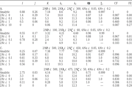
TABLE 3

Comparison of simulation and analytic results forε⬎0

I J K kA kB φ2 ␳2 CF FE

A. 2N␣ ⫽500, 2N␤ ⫽2N␥ ⫽300, 4Nu⫽0.05, 4Nv⫽0.2

Analytic 0.88 0.26 7.18 8.6 9.2 0.98 0.997 1 0

2Nc⫽0 1.4 0.39 7.4 10.0 11.2 0.87 1.0 0.987 0.004 2Nc⫽0.1 1.5 0.6 5.3 9.9 11.3 0.94 1.0 0.894 0.015

2Nc⫽1 0.5 0.06 0.6 9.2 11.4 0.86 1.0 0.460 0.080

2Nc⫽10 0 0 0.06 9.2 11.4 — — 0.087 0.279

B. 2N␣ ⫽100, 2N␤ ⫽2N␥ ⫽60, 4Nu⫽0.05, 4Nv⫽0.2

Analytic 0.55 0.17 3.32 4.21 4.60 0.96 0.99 1 0

2Nc⫽0 1.4 0.1 2.5 4.7 6.1 0.88 1.0 0.967 0.011

2Nc⫽0.1 0.78 0.28 2.4 5.3 6.3 1.0 1.0 0.883 0.036

2Nc⫽1 0 0 0 4.9 6.1 — — 0.183 0.310

C. 2N␣ ⫽500, 2N␤ ⫽2N␥ ⫽450, 4Nu⫽0.05, 4Nv⫽0.2

Analytic 0.25 0.07 7.38 7.77 7.95 0.997 0.999 1 0 2Nc⫽0 0.89 0.17 8.1 9.4 10.2 0.91 0.67 0.996 0.002 2Nc⫽0.1 0.61 0.33 6.8 8.6 9.2 0.90 1.0 0.962 0.005 2Nc⫽1 0.61 0.39 3.5 9.3 10.0 0.90 1.0 0.732 0.037

2Nc⫽5 0.56 0 0.11 10.5 12.1 1 — 0.096 0.201

D. 2N␣ ⫽500, 2N␤ ⫽475, 2N␥ ⫽50, 4Nu⫽4Nv⫽0.2

Analytic 2.75 0.03 4.14 7.0 10.5 0.71 0.999 1 0

2Nc⫽0 3.3 0 4.4 8.1 12.6 0.67 — 0.980 0.002

2Nc⫽0.1 2.0 0.06 3.2 7.8 12.3 0.61 1.0 0.830 0.019

2Nc⫽1 0.11 0 0.28 5.8 12.9 1.0 — 0.384 0.112

2Nc⫽5 0 0 0 5.4 12.3 — — 0.108 0.292

In all simulations N⫽5000. Each set of parameter values was run for 200,000 generations and data were accumulated every 10,000 generations beginning in generation 30,000.

that can be created by recombination, depending on

j⬎ 1

␤

冢

␣␥

␣ ⫺ ␤⫹ ␤ ⫺ ␣

冣

. (23a)

the common haplotypes the A and B alleles are in, but the analysis of each case is not difficult. To illustrate,

Similarly, if the A allele of the rare haplotype is in a let ␰ be the frequency of a rare haplotype containing

unique haplotype and the B allele is in a class i multi-A alleles at both loci that are otherwise found in unique

haplotype, then the rare haplotype will increase in fre-haplotypes. For example, if the rare haplotype is A1B1,

quency if and, at the equilibrium being analyzed, A1is in a unique

haplotype with some other B, say B2, and B1 is in a

i⬎1

␥

冢

␣␤

␣ ⫺ ␥⫹ ␥ ⫺ ␣

冣

. (23b)

unique haplotype with some other A, say A2, it is easy to show that A1B1will decrease in frequency ifε⬎0 and

will increase in frequency if the inequality is reversed. _{These two conditions imply thatε⬎0 is not sufficient} In a similar way, the conditionε⬎0 ensures that the for (4) to be locally stable. For (23a) and (23b) to be recombinant haplotype will decrease in frequency when satisfied for iⱖ2 and jⱖ2, both␤and␥must be close the A allele is otherwise in a unique haplotype and the to ␣. For example, if ␣ ⫽ 0.05, ␤ ⫽ ␥ ⫽ 0.03 (Table B allele is otherwise in a class j multi-B haplotype, or 3A), then the right-hand sides of (23a and b) are both when the B allele is in a unique haplotype and the A 1.83. If, instead,␤ ⫽ ␥ ⫽0.045 (Table 3C), the critical allele is in a class i multi-A haplotype. The same result values of i and j increase to 3.08. In general, larger also holds when the A allele of the rare haplotype is in values ofεpermit local stability of (4) for larger values a class i multi-A haplotype and the B allele is in a class of i and j, but only with very large values of␣are much

j multi-B haplotype. larger values of i and j possible in a stable equilibrium.

However, local stability is not guaranteed by ε ⬎ 0 If␤is close to␣but␥is quite small, the range of values for the other noncomplementary haplotypes. For exam- of i and j for which (4) is stable is also restricted. For ple, if the B allele of the rare haplotype is in a unique example, with ␣ ⫽ 0.05, ␤ ⫽ 0.0475, and ␥ ⫽ 0.005 haplotype and the A allele is in a class j multi-B haplo- (Table 3D), the right-hand sides of (23a) and (23b) are

These results suggest that the complementary equilib- chosen at random without replacement from each data ria predicted when c⫽0 are not of biological interest set for comparison with the data shown in Table 1, and because they are not locally stable. Simulation results in those cases a minimum value of 2 was used, as in the presented below show otherwise. With very low recombi- analysis of the data in Table 1.

nation rates, recombinant haplotypes that could destabi- Positive epistasis:Ifε⬎0, the simulation results can lize the equilibrium appear only very infrequently, and be compared to predictions from the analytic theory. their rate of increase when rare is very small, meaning Some results are shown in Table 3. For c⫽0, the simula-that they would have a very small chance of becoming tion results agree roughly with the analytic predictions. common. As a consequence, complementary equilibria When the threshold haplotype number is 100, there will be found in finite populations even if they would tend to be slightly more multi-A and multi-B haplotypes be unstable in infinitely large populations. than predicted. If that threshold is raised to 200, the simulation results are slightly different. For example, in Table 3A, if a threshold value of 200 copies is used, the SIMULATION RESULTS _{averages of I, J, and K in the simulations for c⫽0 are}

0.89, 0.39, and 8.2, respectively. The predictions of the approximate theory were

com-When c is of the same order of magnitude as u and pared with those from a computer simulation of the

v, the simulation results are still similar to analytic

pre-same model. The computer model used a rejection

dictions. That is consistent with the Karlin and scheme to simulate overdominant selection. In all cases

McGregor(1972) theory. When c is an order of magni-shown in the tables, a population size of N⫽5000 was

tude larger than u and v, the simulation results no used. For each set of parameter values, samples from

longer agree with the analytic theory. Fewer comple-the population were taken every 10,000 generations,

mentary haplotypes remain. Nevertheless, there is still beginning in generation 30,000 and continuing to

gen-substantial linkage disequilibrium present, many of the eration 200,000. Results presented in the tables are

val-possible haplotypes are still not found in appreciable ues averaged over those 18 samples. Other simulations

frequencies, and many complementary haplotypes are showed that this sampling scheme was sufficient to

ob-still present. tain results close to those from simulations carried out

Negative epistasis: If ε ⬍ 0, the analytic theory no

for much longer times.

longer provides an approximate solution but it does In the calculation of the various statistics shown, it

suggest what will be seen. Even without recombination, was necessary to choose a minimum number of copies

some mutations in multi-A or multi-B haplotypes can of a haplotype counted as a common haplotype. The

generate noncomplementary haplotypes that will not results shown in Tables 3 and 4 are for the entire

popula-be eliminated by selection. For example, if for a class tion. Haplotypes were counted in the analysis only if

2 multi-A haplotype, A1B1and A1B2, an A1in A1B1mutates ⬎100 copies were present in the population. That

num-to A*, A*B1 has a chance of increasing in frequency ber is less than the number of haplotypes expected at

to become common but A1B1 will not be eliminated. the deterministic equilibrium frequencies Equation 4,

However, A1B1is still liable to be lost because of drift, which were in the range 0.01–0.04 for the parameter

so complementarity can be restored. Although the solu-values used in Tables 3 and 4. As discussed below, the

tion for the deterministic equilibrium in that case can-choice of that minimum number affects the results

not be obtained in a simple form, it is easy to see that somewhat but does not change the overall patterns

found. In Table 5, samples of 253 chromosomes were the frequency of A1B1 at the deterministic equilibrium

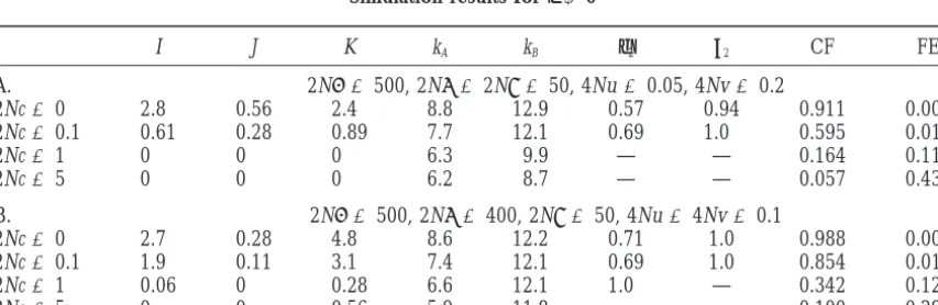
TABLE 4

Simulation results forε⬍0

I J K kA kB φ2 ␳2 CF FE

A. 2N␣ ⫽500, 2N␤ ⫽2N␥ ⫽50, 4Nu⫽0.05, 4Nv⫽0.2

2Nc⫽0 2.8 0.56 2.4 8.8 12.9 0.57 0.94 0.911 0.002 2Nc⫽0.1 0.61 0.28 0.89 7.7 12.1 0.69 1.0 0.595 0.019

2Nc⫽1 0 0 0 6.3 9.9 — — 0.164 0.112

2Nc⫽5 0 0 0 6.2 8.7 — — 0.057 0.432

B. 2N␣ ⫽500, 2N␤ ⫽400, 2N␥ ⫽50, 4Nu⫽4Nv⫽0.1

2Nc⫽0 2.7 0.28 4.8 8.6 12.2 0.71 1.0 0.988 0.005

2Nc⫽0.1 1.9 0.11 3.1 7.4 12.1 0.69 1.0 0.854 0.018

2Nc⫽1 0.06 0 0.28 6.6 12.1 1.0 — 0.342 0.123

is lower than the frequencies of either A*B1 or A1B2 the cases in whichε⬎ 0 and␤and␥ are comparable because it forms single homozygotes with both of them, in magnitude, including those shown in Table 3, A–C, and hence A1B1will have a higher rate of loss by drift. predict those patterns. The cases shown in Table 3D and The magnitude of this effect cannot be predicted but in Table 4 are similar enough to provide an adequate we can expect that substantial complementarity can be comparison with Table 1.

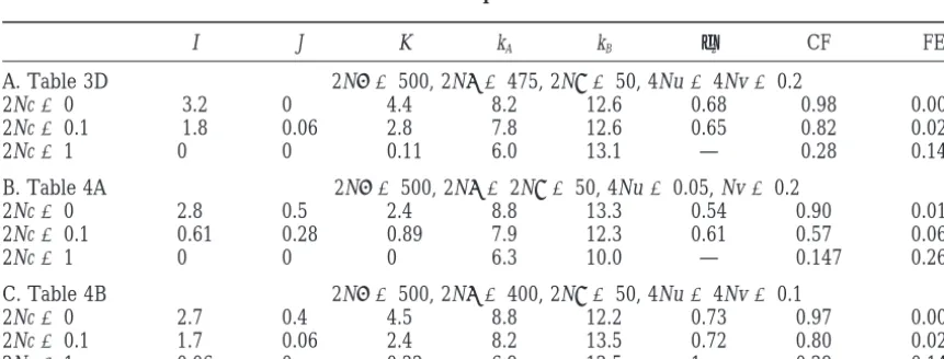
found ifε⬍0 and that a higher degree of complemen- Table 5 shows that many of the features found in the tarity will be found ifεis negative but small in absolute data in Table 1 can be reproduced by this model. Values value. These patterns are seen in Table 4 for c⫽ 0. of c of the same order of magnitude as the mutation For cases with ε ⬍ 0 and c ⬎ 0, the Karlin and rates give the closest agreement. Ifεis positive (Table McGregor (1972) theory is not useful for predicting 5A) or only slightly negative (Table 5C), strong asymme-patterns found in the simulations. Ifε⬍0, a completely _{try in selection on the single homozygotes (␤ Ⰷ ␥) is} complementary deterministic equilibrium with linkage required, but ifεis much⬍0, then a modest asymmetry disequilibrium is unstable to invasion by recombinant in mutation rates (Table 5B, with v ⫽ 4u) produces haplotypes, so the Karlin-McGregor theory predicts that similar results even with ␤ ⫽ ␥. In all these cases, we such an equilibrium should be structurally unstable to see differences in the numbers of alleles maintained, increases in c from 0. That is not seen in the simulation _{0 or nearly 0 values of J, relatively small values of φ2} results. Extensive linkage disequilibrium is found for (indicating relatively large values ofφi for i⬎ 2), and small values of c even whenεis relatively large in abso- values of both CF and FE that are roughly comparable lute value (ε⫽ ⫺0.04 in Table 4A). The loss of comple- to those found in the data. The simulation results differ mentarity with increasing c is more rapid than in the _{from Table 1 by predicting nearly the same values of I} cases withε⬎ 0, because selection is no longer acting _{and K, while in Table 1, I⫽2 and K⫽0.}

to maintain it. But the observation of substantial linkage _{For the data of Sauermann (1998) for the rhesus} disequilibrium and relatively high complementarity _{monkey, the pattern is very different. All 14 haplotypes} does not imply that εis positive. _{are unique haplotypes, so K⫽14, I⫽J⫽0, and there}

Small sample sizes:The simulation results shown in _{is perfect complementarity (CF⫽1) and no extra}

haplo-Tables 3 and 4 were chosen to illustrate the patterns _{types (FE⫽0). That pattern is found ifεis positive and} found in the whole population. I do not consider the _{relatively large, which means that␤and␥are} compara-general sampling problem but present results for sam- _{ble in magnitude and each nearly as large as␣, and if} ples of the same size as in Table 1, to determine what _{c is very small.}

kinds of selection are consistent with these observations. We can restrict our attention to cases that exhibit some of the general features of the data in Table 1, particularly

DISCUSSION AND CONCLUSIONS the difference in the numbers of alleles at the two loci,

This article has three goals. The first is to present new the relatively small number of haplotypes found, the

ways of quantifying the pattern of linkage disequilibrium high degree of complementarity, and the presence of

multi-A but no multi-B or unique haplotypes. None of between two multiallelic loci when there is obvious

sig-TABLE 5

Simulation results for samples of 253 chromosomes

I J K kA kB φ2 CF FE

A. Table 3D 2N␣ ⫽500, 2N␤ ⫽475, 2N␥ ⫽50, 4Nu⫽4Nv⫽0.2

2Nc⫽0 3.2 0 4.4 8.2 12.6 0.68 0.98 0.003

2Nc⫽0.1 1.8 0.06 2.8 7.8 12.6 0.65 0.82 0.021

2Nc⫽1 0 0 0.11 6.0 13.1 — 0.28 0.145

B. Table 4A 2N␣ ⫽500, 2N␤ ⫽2N␥ ⫽50, 4Nu⫽0.05, Nv⫽0.2

2Nc⫽0 2.8 0.5 2.4 8.8 13.3 0.54 0.90 0.018

2Nc⫽0.1 0.61 0.28 0.89 7.9 12.3 0.61 0.57 0.069

2Nc⫽1 0 0 0 6.3 10.0 — 0.147 0.268

C. Table 4B 2N␣ ⫽500, 2N␤ ⫽400, 2N␥ ⫽50, 4Nu⫽4Nv⫽0.1

2Nc⫽0 2.7 0.4 4.5 8.8 12.2 0.73 0.97 0.007

2Nc⫽0.1 1.7 0.06 2.4 8.2 13.5 0.72 0.80 0.024

2Nc⫽1 0.06 0 0.22 6.9 12.5 1 0.29 0.146

nificant nonrandom association between them. The sec- for the possibility that some alleles may carry intrinsic disadvantages, as modeled bySlatkinandMuirhead ond is to develop an approximate analytic model that

accounts for selection and mutation at two multiallelic (1999), and no possibility that mutation rates to differ-ent alleles or classes of alleles at each locus might differ. loci in a finite population. The third is to determine

the extent to which a simple highly symmetric model The goal in comparing data to theory is to see how good the predictions of this simple model are and where of selection can account for patterns found in data from

the DQA1 and DQB1 loci in the MHC regions of hu- apparent differences lie.

ForSauermann’s (1998) data for the rhesus monkey, mans and nonhuman primates.

Quantifying the extent of disequilibrium when there the theory fits the data well provided that selection is strong, the fitnesses of the single-locus homozygotes are is strong balancing selection requires new approaches

because it is not enough to show that there is significant comparable and nearly as small as the fitnesses of the double homozygotes, and the recombination rate is low, disequilibrium. In many cases, linkage disequilibrium

is so apparent that statistical tests are unnecessary. The not much larger than the mutation rates to functionally different alleles at each locus. The agreement between problem instead is to distinguish between the many

kinds of patterns that could be found. The approach theory and data does not mean that the model’s assump-tions are valid for DQA1 and DQB1 in rhesus monkeys, taken here is based on the theoretical result that with

very low recombination rates, selection, mutation, and only that no additional assumptions are necessary to account for the observations.

drift will together create and maintain

complementar-ity, with relatively few haplotypes found in appreciable The fit of the model’s predictions to the data in Table 1 is less good. Many of the features can be reproduced numbers and many or most of them having Lewontin’s

D⬘ ⫽ 1. That theoretical result suggests that FE and by the model but it does not seem possible to predict more multi-A haplotypes than unique haplotypes. That CF indicate how close to complete complementarity a

particular data set is. If high complementarity is found, difference would probably require a more complex model of selection that embodied the functional restric-then the numbers of alleles at one locus in haplotypes

with each allele at the other locus, measured by I, J, K, tions of the type found by Kwok et al. (1993). Still,

the parameter values needed to achieve the degree of φi, and␳j, are of interest because their values are

pre-dicted by the analytic model. asymmetry found in the data all have in common that one or both of the single-locus homozygotes must have The analytic model predicts the simulation results

with reasonable accuracy when there is positive epistasis a fitness comparable to the double homozygote. Not enough is known about the effect of these two loci on (ε⬎0) and low rates of recombination. When there is

positive epistasis, one of two patterns is found. If the fitness to know whether that is true for DQA1 and DQB1 in humans, but at least the model does suggest that fitnesses of the single-locus homozygotes are

compara-ble (␤and␥have similar magnitudes), then at an equi- there are differences in the fitness interactions between these loci in humans and in the rhesus monkey. librium, most haplotypes are unique and roughly equal

numbers of alleles are found at both loci even if muta- For chimpanzees and gorillas, Gyllensten and Erlich(1993) found no significant linkage disequilib-tion rates differ. Only if one of the single-locus

homozy-gotes is much less fit than the other (␤ Ⰷ ␥, but still with rium. They suggested that either the recombination rate is much higher or selection is weaker than in humans. ε⬎0) are the results asymmetric, with an appreciable

number of multi-A or multi-B haplotypes and a substan- The theory described here supports that view but shows that differences in either of these parameters would tial difference in the numbers of alleles at the two loci.

If ε⬍ 0, the analytic model can no longer be used have to be by an order of magnitude or more. Small differences from the values in humans would not be but the development of that model suggests that nearly

complete complementarity will be found for small sufficient to eliminate linkage disequilibrium. A differ-ence in effective population size could not account for enough recombination rates. Simulation results

con-firmed that prediction, but with two differences from the patterns observed, because both the recombination rates and selection coefficients are scaled by the same the cases withε⬎ 0. Recombination is more effective

in destroying complementarity and differences in the factor, so the relative intensities of selection and recom-bination would remain the same.

mutation rates can more easily lead to asymmetry of the

results. These conclusions about the action of selection at

DQA1 and DQB1 have to be regarded as tentative be-Both the analytic and simulation models are not

in-tended to provide a complete description of DQA1 and cause there are too few population-level studies of haplo-type frequencies in populations of humans and nonhu-DQB1 or any other pair of loci. The model was designed

to have as few parameters as possible. Selection is highly man primates to know whether those patterns are found in other populations as well. The data are discussed to symmetric, with the many possible genotypes grouped

into only four fitness classes. There are no specific inter- illustrate the application of the theory and to show that population-level data can be used to test hypotheses actions among alleles, as has been demonstrated for

Hill, W. G.,andA. Robertson,1968 Linkage disequilibrium in I thank S. McWeeney for providing information and references _{finite populations. Theor. Appl. Genet. 38: 226–231.}

about linkage disequilibrium in DQA and DQB and M. W. Feldman, Karlin, S.,andM. W. Feldman,1970 Linkage and selection: two S. McWeeney, and G. Thomson for helpful discussions and advice. locus symmetric viability model. Theor. Popul. Biol. 1: 39–71.

Karlin, S.,andJ. L. McGregor,1972 Polymorphisms for genetic This research was supported in part by National Institutes of Health

and ecological systems with weak coupling. Theor. Popul. Biol. grant GM-40282.

3:210–238.

Kimura, M.,andJ. F. Crow,1964 The number of alleles that can be maintained in a finite population. Genetics 49: 725–738.

Kwok, W. W., S. Kovats, P. ThurtleandG. T. Nepom,1993 HLA-DQ allelic polymorphisms constrain patterns of class II

hetero-LITERATURE CITED

dimer formation. J. Immunol. 150: 2263–2272.

Begovich, A. B., G. R. McClure, V. C. Suraj, R. C. Helmuth, N. _{Lewontin, R. C.,1964 The interaction of selection and linkage. I.} Fildeset al., 1992 Polymorphism, recombination, and linkage _{General considerations; heterotic models. Genetics 49: 49–67.} disequilibrium within the HLA class II region. J. Immunol. 148: _{Lewontin, R. C.,andK. Kojima,1960 The evolutionary dynamics} 249–258. of complex polymorphisms. Evolution 14: 458–472.

Bengtsson, B. O.,andG. Thomson,1981 Measuring the strength Marsh, S. G.,1998 HLA class II region sequences, 1998. Tissue of associations between HLA antigens and diseases. Tissue Anti- Antigens 51: 467–507.

gens 18: 356–363. Nagylaki, T., 1992 Introduction to Theoretical Population Genetics.

Christiansen, F. B.,andM. W. Feldman,1975 Selection in complex Springer-Verlag, New York.

Peterson, A. C., A. Di Rienzo, A. E. Lehesjoki, A. de la Chapelle,

genetic systems. IV. Multiple alleles and interactions between two

M. Slatkinet al., 1995 The distribution of linkage disequilib-loci. J. Math. Biol. 2: 179–294.

rium over anonymous genome regions. Hum. Mol. Genet. 4:

Cullen, M., J. Noble, H. Erlich, K. Thorpe, S. Becket al., 1997

887–894. Characterization of recombination in the HLA class II region.

Sasaki, A., 1989 Evolution of pathogen strategies. Ph.D. Thesis, Am. J. Hum. Genet. 60: 397–407.

Biology, Kyushu University, Fukuoka, Japan.

Ewens, W. J.,1979 Mathematical Population Genetics. Springer-Verlag,

Sasaki, A.,1992 The evolution of host and pathogen genes under New York.

epidemiological interaction, pp. 247–263 in Population

Paleo-Feldman, M. W., R. C. Lewontin, I. R. FranklinandF. B.

Christian-Genetics, edited byN. Takahata.Japan Scientific Society Press,

sen,1975 Selection in complex genetic systems. III. An effect

Tokyo. of allele multiplicity with two loci. Genetics 79: 333–347.

Sauermann, U.,1998 DQ-haplotype analysis in rhesus macaques:

Fernandez-Vin˜ a, M. A., X. J. Gao, M. E. Moraes, J. R. Moraes, I.

implications for the evolution of these genes. Tissue Antigens

Salatielet al., 1991 Alleles at four HLA class II loci determined

52:550–557. by oligonucleotide hybridization and their associations in five

Slatkin, M.,andC. A. Muirhead,1999 Overdominant alleles in a ethnic groups. Immunogenetics 34: 299–312.

population of variable size. Genetics 152: 775–781.

Gillespie, J. H.,1984 Some properties of finite populations

experi-Takahata, N., 1990 A simple genealogical structure of strongly encing strong selection and weak mutation. Am. Nat. 121: 691–

balanced allelic lines and trans-species evolution of polymor-708. _{phism. Proc. Natl. Acad. Sci. USA 87: 2419–2423.}

Grahovac, B., R. I. Sukernik, C. O’Huigin, Z. Zaleska-Rutczynska, _{Vekemans, X.,andM. Slatkin,1994 Gene and allelic genealogies} N. Blagitkoet al., 1998 Polymorphism of the HLA class II loci _{at a gametophytic self-incompatibility locus. Genetics 137: 1157–} in Siberian populations. Hum. Genet. 102: 27–43. _1165.

Griffiths, R. C., 1981 Neutral two-locus multiple alleles models _{Wolfram, S., 1996 The Mathematica Book. Wolfram Media Inc.,} with recombination. Theor. Popul. Biol. 19: 169–186. _{Champaign, IL.}

Gyllensten, U. B.,andH. A. Erlich,1993 MHC class II haplotypes