COLSON, THOMAS PAYTON. STREAM NETWORK DELINEATION FROM HIGH-RESOLUTION DIGITAL ELEVATION MODELS. (Under the direction of Professor James D. Gregory.)
by
THOMAS PAYTON COLSON
A dissertation submitted to the Graduate Faculty of North Carolina State University
in partial fulfillment of the requirements for the Degree of
Doctor of Philosophy
FORESTRY
Raleigh, North Carolina
2006
Approved By:
Dr. Helena Mitasova Dr. Montserrat Fuentes
Biography
Contents
List of Figures vii
List of Tables x
1 Introduction 1
1.1 Background . . . 2
1.2 Research Approach . . . 2
1.2.1 Objective 1: Collect Field Data . . . 3
1.2.2 Objective 2: Determine Extent of Accuracy of Available Stream Maps . . . 4
1.2.3 Objective 3: Evaluate Sources of DEMs . . . 4
1.2.4 Objective 4: Stream Extraction Evaluation. . . 4
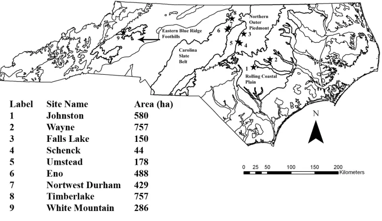
1.3 Study Sites . . . 5
1.4 References Cited . . . 7
2 Headwater Streams: A Review of the Literature 9 2.1 Headwater Streams: Definitions and Functions . . . 10
2.2 Field Identification of Streams . . . 10
2.3 Headwater Stream Sources . . . 14
2.4 Function of Headwater Streams. . . 15
2.4.1 Headwater Streams Form Channels . . . 16
2.4.2 Headwater Streams Move Sediment . . . 16
2.4.3 Headwater Streams Host Unique Biota . . . 17
2.5 Impacts of Disturbances to Stream Networks . . . 21
2.5.1 Impervious Surface (Hydrologic Alteration) . . . 21
2.5.2 Sedimentation . . . 24
2.5.3 Nutrient Loading . . . 27
2.6 Stream Management Regulatory Programs . . . 29
2.6.1 Federal Regulation . . . 30
2.6.2 North Carolina Regulation . . . 31
3 Stream Map Accuracy: A Review of the Literature 49
3.1 Abstract . . . 50
3.2 Introduction . . . 51
3.2.1 Headwater Stream Channel Representation on Topographic Maps . . . 52
3.2.2 Stream Representation Standards . . . 57
3.2.3 Impact of Cartographic Generalization . . . 58
3.2.4 Digital Stream Maps . . . 59
3.2.5 Calculation of Hydrologic Indices Using Blue Lines . . . 61
3.3 Conclusion . . . 65
3.4 Acknowledgments . . . 67
3.5 References Cited . . . 68
4 Mobile GIS 78 4.1 Abstract . . . 79
4.2 Introduction . . . 80
4.3 System Design . . . 84
4.4 System Application . . . 93
4.5 Conclusion . . . 97
4.6 Acknowledgements . . . 99
4.7 References Cited . . . 99
5 Accuracy and Completeness of Stream Maps 104 5.1 Abstract . . . 105
5.2 Introduction . . . 106
5.3 Methods . . . 110
5.3.1 Data Acquisition . . . 111
5.3.2 GPS Stream Survey. . . 112
5.3.3 National Hydrography Dataset Flowlines . . . 112
5.3.4 North Carolina Floodplain Mapping Program Surface Water Lines . . . 113
5.3.5 NRCS Soil Map Stream Lines . . . 113
5.3.6 County Data . . . 115
5.3.7 Assessment of Horizontal Accuracy . . . 116
5.3.8 Network Indices . . . 120
5.4 Results. . . 120
5.4.1 Horizontal Accuracy of Stream Maps . . . 122
5.4.2 Stream Network Completeness . . . 125
5.5 Discussion . . . 128
5.5.1 Horizontal Accuracy of County GIS Stream Lines . . . 128
5.5.2 Horizontal Accuracy of NRCS Soil Map Stream Lines . . . 129
5.5.3 Horizontal Accuracy of NCFMP Surface Water Lines . . . 130
5.5.4 Horizontal Accuracy of NHD Flowlines . . . 130
5.5.5 Completeness . . . 131
5.6 Conclusion . . . 133
5.7 Acknowledgments . . . 135
6 Extraction and Delineation 139
6.1 Abstract . . . 140
6.2 Introduction . . . 141
6.2.1 USGS DEMs . . . 142
6.2.2 LiDAR DEMs . . . 143
6.2.3 Creation of DEMs . . . 144
6.2.3.1 Kriging. . . 144
6.2.3.2 RST . . . 145
6.2.3.3 ANUDEM . . . 146
6.2.4 Effects of DEM Resolution on Terrain Analysis . . . 147
6.2.5 Spurious Depressions . . . 148
6.2.5.1 Treatment of Spurious Depressions in DEMs . . . 148
6.2.5.2 Breaching . . . 149
6.2.5.3 Impact Reduction Approach. . . 150
6.2.6 Flow Direction . . . 151
6.2.6.1 Single Flow Direction . . . 151
6.2.6.2 Multiple Flow Direction . . . 152
6.2.7 EDNA. . . 153
6.3 Objectives . . . 153
6.4 Methods . . . 154
6.4.1 Experimental Design and Statistical Analysis . . . 154
6.4.1.1 Digital Stream Networks . . . 155
6.4.1.2 Ground Truth Stream Networks . . . 156
6.4.1.3 Statistical Analysis . . . 157
6.4.2 Description of Study Site Locations . . . 157
6.4.3 Stream Surveying . . . 158
6.4.4 DEM Blocks . . . 159
6.4.4.1 Interpolation of LiDAR Data to Create DEMs . . . 159
6.4.4.2 USGS and NCFMP DEMs . . . 161
6.4.5 DEM Treatment . . . 161
6.4.6 Extraction of Stream Networks. . . 162
6.4.6.1 TAUDEM . . . 162
6.4.6.2 Arc Hydro . . . 163
6.4.7 Accuracy Determination . . . 165
6.5 Results. . . 168
6.5.1 ANUDEM Interpolation . . . 168
6.5.2 Stream Extraction. . . 170
6.5.3 Coastal Plain . . . 170
6.5.3.1 Johnston County Study Site . . . 171
6.5.3.2 Wayne County Site . . . 173
6.5.4 Carolina Slate Belt . . . 176
6.5.4.1 Timberlake . . . 177
6.5.4.2 Eno. . . 180
6.5.5 Northern Outer Piedmont. . . 183
6.5.5.1 Falls Lake . . . 184
6.5.5.2 Schenck Forest. . . 185
6.5.5.3 Umstead State Park . . . 186
6.5.6 Eastern Blue Ridge Foothills . . . 187
6.5.6.1 White Mountain . . . 187
6.6 Statistical Analysis of the Results. . . 189
6.6.1 Interaction Effects of DEM Source and Depression Removal Method . . . 190
6.6.2 Main Effects . . . 192
6.6.3 Differences Among Depression-Removal Methods . . . 193
6.6.4 Differences Among DEM Sources . . . 196
6.7 Discussion . . . 198
6.7.1 Block (DEM) Effect . . . 198
6.7.1.1 USGS 10m DEMs . . . 199
6.7.1.2 NCFMP 6.10 m DEMs . . . 199
6.7.1.3 Interpolated DEMs . . . 200
6.7.2 Treatment (Depression-Removal Method) Effect . . . 201
6.7.3 Comparison to Published Stream Maps . . . 203
6.7.3.1 NCFMP Surface Water Lines . . . 203
6.7.3.2 Soil Maps . . . 206
6.7.3.3 National Hydrography Dataset . . . 208
6.7.3.4 County GIS Streams . . . 210
6.8 Conclusion . . . 212
6.9 References Cited . . . 215
6.10 Appendix . . . 228
List of Figures
3.1 Stream omission error on USGS topographic maps, Shining Rock (North) and
Ros-man (South) Quadrangle, NC. . . 61
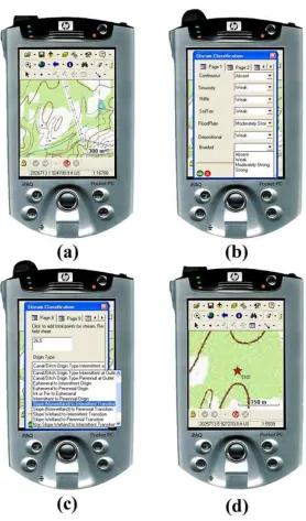
4.1 Stream ID application: (a) topographic map background, (b) attributing stream
ori-gin features, (c) determining oriori-gin type, and (d) labeled stream oriori-gin. . . 89
5.1 Stream location error on USGS topographic map. . . 109
5.2 Locations of study catchments relative to EPA Level IV Ecoregion. . . 111
5.3 Scanned soil map showing locations of the stream network at Schenck Forest in
Raleigh, NC. . . 114
5.4 Measuring distances of surveyed stream channel points from NHD flowlines. . . . 117
5.5 Multiple buffer ring analysis of blueline accuracy. . . 119
5.6 GPS surveyed streams at Timberlake study site compared to Soil Map (a), NHD (b),
NCFMP (c), and Person County GIS (d). . . 121
5.7 Number of GPS survey points within buffer distance classes for related GIS stream
segments only. County GIS stream lines (a), NCFMP surface water lines (b), NHD
Flowlines (c), and NRCS soil map stream lines (d). . . 125
5.8 NCFMP surface water lines and NHD flowlines in Person County, NC.. . . 131
6.1 Locations of study catchments relative to EPA Level IV Ecoregion. . . 156
6.2 Flowchart showing major steps in DEM acquisition, interpolation, conditioning, and
extraction process. . . 164
6.3 Example showing GPS points within each of a series of buffers drawn around a
mapped stream line. . . 167
6.4 Scatterplots showing effects of TOPOGRID parameter values on percent of GPS
points 3.05 m from a mapped channel, Johnston County site: roughness penalty (a), discrete error factor (b), vertical standard error (c) and, 3-way plot of all parameters (d).. . . 169
6.5 Mean percentage of GPS points 3.05 m from all mapped streams in the Coastal
Plain by (a) treatment and (b) block. . . 171
6.6 Sensitivity of depression-removal methods to flat and swampy terrain on a 1.52 m
resolution DEM interpolated with ANUDEM: a) Arc Hydro and constrained
6.7 Streams extracted from DEMs treated with impact reduction approach: a) 3.05 m resolution DEM and USGS 10 m DEM and b) 6.10 m resolution DEM and NCFMP DEM. . . 173
6.8 Comparison of depression-removal methods encountering a man-made obstacle on
a 3.05 m resolution DEM interpolated with ANUDEM, Wayne County, NC: a) con-strained breaching, b) impact reduction approach, c) Planchon and Darboux, and d)
slow breaching. . . 174
6.9 Comparison of depression-removal methods encountering a beaver pond and swamp
complex on a 3.05 m resolution DEM interpolated with ANUDEM, Wayne County, NC: a) slow breaching and Arc Hydro and b) constrained breaching and impact
reduction approach. . . 175
6.10 Mean percentage of GPS points 3.05 m from all mapped stream in the Carolina
Slate Belt by (a) treatment and (b) block. . . 176
6.11 Sensitivity of depression-removal methods to a large man-made obstruction (cul-vert) at the Timberlake site on a 1.52 m resolution DEM interpolated with ANU-DEM: a) slow breaching, constrained breaching, and Planchon and Darboux and b)
Arc Hydro and impact reduction approach . . . 178
6.12 Timberlake DEM showing affects of depression-removal methods on 1.52 m resolu-tion DEM: a) constrained breaching, b) impact reducresolu-tion approach, c) slow
breach-ing and d) Planchon and Darboux. . . 179
6.13 Comparison of depression-removal methods at the Northwest Durham site on a 1.52 m resolution DEM interpolated with ANUDEM: a) Arc Hydro and constrained breaching and b) impact reduction approach, Planchon and Darboux, and slow
breaching. . . 181
6.14 Effect of grid cell size on ability of impact reduction approach DEM treatment to “carve” a channel at the Northwest Durham study site: a) 1.52 m TG, b) 3.05 m TG,
c) 6.05 m NCFMP, and d) 10 m USGS DEM. . . 182
6.15 Mean percentage of GPS points 3.05 m from all mapped stream in the Northern
Outer Piedmont by (a) treatment and (b) block. . . 183
6.16 Comparison of various Falls Lake DEMs treated with impact reduction approach:
a) IRA 1.52, 3.05, and 6.10 m and b) USGS 10 m and NCFMP 6.10 m.. . . 184
6.17 Comparison of various Schenck Forest DEMs treated with slow breaching: a) IRA
1.52, 3.05, and 6.10 m and b) USGS 10 m and NCFMP 6.10 m.. . . 185
6.18 Comparison of various Umstead State study site DEMs treated with constrained
breaching: a) IRA 1.52, 3.05, and 6.10 m and b) USGS 10 m and NCFMP 6.10 m. 186
6.19 Mean percentage of GPS points 3.05 m from all mapped stream in the Eastern Blue
Ridge Foothills by (a) treatment and (b) block.. . . 187
6.20 Comparison of slow breaching treatment on two DEM blocks for the White
Moun-tain study site: a) SB and IRA 1.52 m and b) SB and IRA NCFMP 6.10 m.. . . 188
6.21 Trend line showing percentage of GPS points in each buffer distance class (TG 3.05
6.22 Interaction plots showing results of treatment (depression-removal method on stream extracted from blocks (DEM source). (a) Johnston and Wayne County sites, (b) Falls Lake, Schenck, and Umstead sites, (c) Eno River, Northwest Durham, and
Timberlake sites and, (d) White Mountain Site. . . 191
6.23 Comparison of NCFMP surface water lines to stream segments extracted from TG 3.05 m resolution DEM treated with impact reduction approach. Wayne (a),
Tim-berlake (b), Johnston (c), and Umstead (d).. . . 205
6.24 Comparison of NRCS soil survey map and TG 1.52 m DEM treated with impact
reduction approach stream networks, Johnston County study site. . . 207
6.25 Comparison of NHD flowlines and TG 1.52 m DEM treated with Arc Hydro and
constrained breaching stream networks, Johnston County study site. . . 209
6.26 Comparison of Wake County GIS stream lines and TG 1.52 m DEM treated with
List of Tables
2.1 Various state forestry agency flow regime definitions. . . 12
2.2 Effects of impervious surface on stream health. . . 22
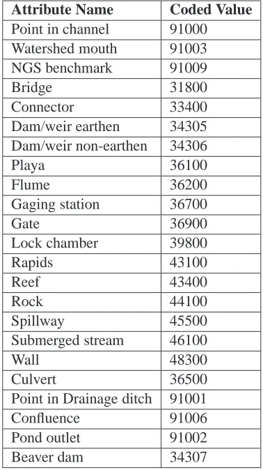
4.1 North Carolina Division of Water Quality Stream Identification Form. Version 3.1 . 85 4.2 Stream Point Attribute Types . . . 90
4.3 Distribution of surveyed stream origins among physiographic sub-regions of NC. . 93
4.4 GPS accuracy estimates . . . 94
5.1 NHD 8-Digit Hydrologic Unit Codes. . . 113
5.2 Accuracy of stream lines on maps, by study site (showing area, number of GPS survey points for that site), reporting percentage of GPS points within 3.05 m buffer for all GPS points and only GPS points with an associated stream. . . 122
5.3 Completeness of stream lines on maps, by study site, showing bias (shows more or less “-” stream links than truth), bifurcation ratio and length ratio. . . 126
6.1 Distribution of surveyed stream origins among physiographic sub-regions of NC. . 159
6.2 Top-performing TOPOGRID parameters. . . 170
6.3 Rolling Coastal Plain ANOVA table (Interaction). . . 191
6.4 Norther Outer Piedmont ANOVA table (Interaction). . . 192
6.5 Carolina Slate Belt ANOVA table (Interaction). . . 192
6.6 Eastern Blue Ridge Foothills ANOVA table (Interaction). . . 192
6.7 Rolling Coastal Plain ANOVA table. . . 193
6.8 Norther Outer Piedmont ANOVA table. . . 193
6.9 Carolina Slate Belt ANOVA table. . . 193
6.10 Eastern Blue Ridge Foothills ANOVA table. . . 193
6.11 Tukey’s HSD test: Rolling Coastal Plain, treatment means. . . 194
6.12 Tukey’s HSD test: Northern Outer Piedmont, treatment means. . . 195
6.13 Tukey’s HSD test: Carolina Slate Belt, treatment means. . . 195
6.14 Tukey’s HSD test: Eastern Blue Ridge Foothills, treatment means. . . 195
6.15 Tukey’s HSD test: Rolling Coastal Plain, block means. . . 197
6.16 Tukey’s HSD test: Northern Outer Piedmont, block means. . . 197
6.17 Tukey’s HSD test: Carolina Slate Belt, block means. . . 197
6.19 Percentage of GPS points within 3.05 m of a mapped channel, Rolling Coastal Plain 229
6.20 Percentage of GPS points within 3.05 m of a mapped channel, Carolina Slate Belt . 230
6.21 Percentage of GPS points within 3.05 m of a mapped channel, Northern Outer Pied-mont . . . 231
6.22 Percentage of GPS points within 3.05 m of a mapped channel, Eastern Blue Ridge
Foothills . . . 232
6.23 Depression Analysis . . . 233
6.24 Percentage of GPS points within 3.05 m of a mapped channel, all stream lines . . . 235
6.25 Buffer distance class, in meter, for which 90% or more of GPS points are within the
Chapter 1
1.1
Background
The current regulatory environment in the State of North Carolina recognizes a stream for planning and administrative purposes only if it exists on a United States Geological Survey (USGS) 1:24,000 scale topographic map or a Natural Resource Conservation Service (NRCS) county soil survey map. These maps are outdated and often inaccurate yet state agencies rely on them to con-duct planning and operations concerning the locations of streams and their potential impact on infrastructure improvements in the state. Beginning in 2000, the North Carolina Floodplain Map-ping Program (NCFMP) acquired Light Detection and Ranging (LiDAR) data and with these data created 6.10 m resolution digital elevation models (DEMs), surface water lines, and flood hazard zones. However, the ability of NCFMP surface water lines to depict the location of headwater streams accurately has not been quantitatively measured. Numerous methods exist for the delin-eation of stream networks from Digital Elevation Models (DEMs). However there is little research that utilizes the high-accuracy and high-resolution characteristics of LiDAR-based DEMs to com-pare stream mapping techniques. High-resolution DEMs such as those created with LiDAR data often contain micro-topographic features such as roads and detention ponds that were not consid-ered during the development of relic stream delineation techniques which are intended for use with coarser-resolution data.
1.2
Research Approach
subre-gions of North Carolina in order to evaluate the feasibility and accuracy of the mapping methodolo-gies across geologic, geomorphologic, and climatic variability. The digital mapping methods were tailored to landscape characteristics of the sampled physiographic subregions and extensive field data were collected to validate mapping methods and products.
1.2.1 Objective 1: Collect Field Data
In each study watershed, the stream networks were surveyed beginning at the mouth and walking every stream reach encountered to the intermittent origin. Survey data were collected with real-time differential global positioning system (GPS) with sub-meter accuracy. The coordinates of specific locations were surveyed using the State Plane Coordinate System (feet):
• Mouth of the watershed
• All tributary junctions
• Random points along stream reaches between tributary junctions to record major changes in direction and the location of the channel
• All stream origins and all transitions among stream types (e.g. intermittent to perennial)
A photographic record of all origins was obtained with a digital camera: two (or more, if appro-priate) photos at each location, upstream and downstream views. A field notebook was kept for each study watershed to record notes on character of the stream network and the characteristics of stream origins and stream type transitions. Stream origins were determined using the latest version of the North Carolina Division of Water Quality (NCDWQ) Stream Identification Form Version 3.1
(NCDWQ,2005). A digital version of the NCDWQ Stream Identification Form was created using
1.2.2 Objective 2: Determine Extent of Accuracy of Available Stream Maps
Streams depicted on USGS, NRCS, NCFMP, and local county maps were assessed using a measure of horizontal accuracy and network completeness. Data used to access these relationships were collected during the GPS survey, and points surveyed within stream channels were attributed with distance from each associated stream map dataset.
1.2.3 Objective 3: Evaluate Sources of DEMs
Grid based DEMs were interpolated from LiDAR elevation points using the Australian National University Digital Elevation Model (ANUDEM) software (Hutchinson, 1989). This ex-tension for ArcMap combines the efficiency of Inverse Distance Weighted (IDW) and Spline inter-polation techniques with the accuracy of Kriging methods (Hutchinson,1993). The program allows the user to specify the vertical standard error of the input data to minimize error in the output DEMs
(Hutchinson and Dowling, 1991). Three “versions” of LiDAR DEMs were interpolated, at 1.52,
3.05, and 6.10 m resolution. DEMs were also obtained from the USGS (10 m resolution) and the NCFMP (6.10 m resolution).
1.2.4 Objective 4: Stream Extraction Evaluation
Multiple software tools incorporating various stream extraction algorithms were compre-hensively compared. The significant variables in these models are thresholds of contributing area and flow direction algorithms. The analysis of pprocessing steps focused on five methods of re-moving artifact depressions in the DEMs. Stream extraction was performed using two off the shelf tools:
simple “point and click” interface for the delineation of watersheds and stream networks using grid DEMs as the only source of input (Maidment,2002).
• TAUDEM (ArcView): Terrain Analysis Using Digital Elevation Models (TAUDEM) is a more comprehensive watershed delineation and stream extraction utility that allows the user to specify parameters such as type of flow direction algorithm to use and method of stream delineation (contributing area threshold, grid order threshold, area and slope threshold, area and length threshold) (Tarboton,1997).
The locations of stream channels predicted via model output were compared to the stream networks surveyed in the nine study watersheds. Modeled stream networks were compared to surveyed stream networks by creating buffers around the modeled streams and classifying surveyed points that fell within 1.52, 3.05, 4.57, 6.10, 7.62, 9.14, 10.67, 12.19, 13.72, 15.24, 16.76, 18.29, 19.81, 21.34, 22.86, 24.38, and 304.80 m buffers around modeled stream networks. The minimum distance, 3.05 meters, represents the theoretical limit of the accuracy of the standard LiDAR DEMs provided publicly by NCFMP at 6.10 m pixel cell resolution (3.05 m on either side of the stream line, drawn through the center of the pixel).
1.3
Study Sites
Nine study watersheds were selected from each of three physiographic subregions of the Mountains, Piedmont and Coastal Plain of North Carolina. The soil systems in North Carolina
(Daniels et al., 1999) and the Environmental Protection Agency (EPA) Level IV Ecoregions of
• Carolina Slate Belt Soil System and Carolina Slate Belt Level IV Ecoregion
• Felsic Crystalline Soil System and Northern Outer Piedmont Level IV Ecoregion
• Middle Coastal Plain Soil System and Rolling Coastal Plain Level IV Ecoregion
• Low and Intermediate Mountain Soil System and Eastern Blue Ridge Foothills Level IV Ecoregion
Selection of the study watersheds was based on the availability of LiDAR data, the availability of control monuments, the representation of diverse stream environments from multiple physiographic regions, and accessibility of the sites for surveying and field data collection. The research focused predominantly on rural landscapes to determine the feasibility of the mapping approaches in stream networks that have not been dramatically altered by urbanization. Ideally, the physiographic sub-regions and study watersheds within subsub-regions should have been randomly selected. However, practical considerations of access to the streams, presence of control monuments, land ownership, etc. required manual selection of study watersheds. Each study watershed was large enough to ensure that:
• The main stream of the watershed and its principal tributaries were depicted on the USGS 1:24,000 scale topographic map and the USGS 1:24,000 scale hydrographic digital line graph (DLG).
• The watershed had a planimetric area of approximately 400-500 ha.
or higher order streams and many of these streams also are not on the maps. The first order streams are those that meet the definitions of intermittent or perennial streams contained in the NC river basin riparian buffer rules (15A NCAC 02B.0233; http://h2o.enr.state.nc.us/admin/rules/rb040103. pdf). The NCDWQ Stream Identification Methodology was used to determine the locations of the origins of first order streams and stream transitions from intermittent to perennial: Identification Methods for the Origins of Intermittent and Perennial Streams (NCDWQ,2005).
1.4
References Cited
Daniels, R. B., Buol, S. W., Kleiss, H. J.,Ditzler, C. A., 1999. Soil Systems in North Carolina. Soil Science Depatrment Technical Bulletin 314, North Carolina State University.
Griffith, G. E., Omernik, J. M., Comstock, J. A., Schafale, M. P., McNab, W. H., Lenat, D. R., MacPherson, T. F., Glover, J. B., Shelburne, V. B., 2002. Ecoregions of North Carolina and South Carolina,(color poster with map, descriptive text, summary tables, and photographs): Reston, Virginia. US Geological Survey (map scale 1: 1,500,000).
Hutchinson, M. F., 1989. A new procedure for gridding elevation and stream line data with auto-matic removal of spurious pits. Journal of Hydrology 106 (3-4), 211–232.
Hutchinson, M. F., 1993. Development of a continent-wide DEM with applications to terrain and climate analysis. In: Goodchild, M. F., Parks, B. O., Steyaert, L. T. (Eds.), Environmental Mod-eling with GIS. Oxford University Press, New York. pp. 392–399
Maidment, D. R., 2002. Arc Hydro: GIS for Water Resources. ESRI Press.
North Carolina Division of Water Quality(NCDWQ), 2005. Indentification methods for the origins of intermittent and perennial streams, version 3.1[Online]. Available at http://h2o.enr.state.nc.us/
ncwetlands/documents/NC Stream ID Manual.pdf. Accessed on June 20 2006.
Chapter 2
Headwater Streams: A Review of the
2.1
Headwater Streams: Definitions and Functions
Headwater streams are the primary sources of water in a drainage network (Stanford,
1996). Headwater stream networks serve as a critical hydrologic link between the surrounding landscape and the larger, connecting stream outflows within a watershed. These networks drain extensive surface areas within the watershed that are not directly in contact with higher order stream channels. These ”headwaters” join together many times forming a continuous hydrologic network consisting of streams, rivers, ponds, lakes, and wetlands.
The literal headwaters of any watershed are the subsurface and overland flow of water dur-ing (and often after) a precipitation event. As runoff water proceeds downslope, it begins to carve out barely discernible ephemeral channels. The location of these temporary stormwater channels is influenced by the topography of the landscape. Groundwater is not an input to ephemeral streams except to those draining wetlands, and they lack the biological, hydrological, and physical charac-teristics commonly associated with the continuous presence of flowing water. Ephemeral channels often transition to intermittent streams, which convey water not only during a storm event but also have baseflow during wetter conditions. Groundwater discharge serves as the predominant source of water input to these channels, however, they frequently dry up during the drier seasons when the groundwater table retreats below the level of the streambed. When groundwater flow is consistent enough to support the continuous flow of water year round, the stream is then defined as perennial
(Harman and Jennings,1999;OEPA,2005).
2.2
Field Identification of Streams
used to determine intermittent and perennial flowing streams (flow regime) for regulatory condi-tions. Many government agencies differentiate between intermittent and perennial streamflow when applying best management practices (BMPs) to land-management strategies. The assumption is that as streamflow duration increases, so does the potential for non-point pollution input and transport by the stream. Correct identification of perennial streams then becomes a critical step in applying BMPs.
Many decision makers rely upon United States Geological Survey (USGS) topographic map “blue lines” for determination of flow regime. Perennial streams are represented by solid blue lines and dashed blue lines are used for intermittent streams. Many government agencies rely solely on this map. Use of blue lines on a USGS topographic map has consistently been shown to be inaccurate for site specific application (Sveca et al.,2005). United States Geological Survey cartographic standards for the depictions of streams on topographic maps state that: 1) all perennial streams, regardless of length, 2) intermittent streams at least 609.6 m (2000 ft) long, and 3) headwater drainages terminate 304.8 m (1000 ft) from the drainage divide (USGS 1980). A West Virginia study showed that the USGS maps identified 12 headwater catchments as intermittent, whereas field observations identified 36 (Paybins,2002).
Table 2.1: Various state forestry agency flow regime definitions.
Agency Perennial Intermittent Citation
North Carolina Di-vision of Forest Re-sources
Flowing water 90% of the time
Flowing water 30 to 90% of the time
(NCDFR,2006)
Kentucky Forest Service
Holds water
throughout the year
Holds water during wet season
(Stringer and
Perk-ings,2001) Tennessee Forest
Service
Flowing water year round
Flowing water 40 to 90% of the time
(TDA,2003)
South Carolina Forestry Commis-sion
Continuously flow-ing water most years
Flowing water from headwater source for portion of year
(SCFC,2006)
Texas Forest Ser-vice
Flowing water 90% of the time
Flowing water 30 to 90% of the time
(TFS,2000)
The USGS has developed a linear regression formula for Massachusetts that accounts for drainage area, drainage density, geology, and basin slope to determine the likelihood of a stream flowing perennially or intermittently (Bent and Archfield, 2002). Hansen(2001) agreed that deci-sion makers should not rely on topographic map blue lines, which he found to depict only 14-21% of the entire stream network, and developed a method for the field determination of intermittent and perennial flow using a combination of geomorphologic and biological indicators.
drainage area contains 75% or more stratified drift deposits, and 3) if no flow is observed for four days the stream is classified as intermittent.
Only a few regulatory agencies combine map-based hydrology characteristics with de-tailed field observations to differentiate between intermittent and perennial flow regimes. These agencies have confirmed that USGS and Natural Resource Conservation Service (NRCS) blue lines depicted on paper maps do not accurately reflect intermittent and perennial transitions. Field indi-cators of hydrological, physical, and biological conditions within the stream are used to determine the likelihood of a stream flowing intermittently or perennially.
The North Carolina Division of Water Quality (NCDWQ) has developed a field protocol in which geomorphologic, hydrologic, and biologic field indicators of stream flow are ranked as 1) “Strong,” 2) “Moderate,” 3) “Weak”’ or 4) “Absent.” The presence and degree of development of each indicator is assigned a numerical value (e.g. “Strong Headcut” would receive a 3, “Absent Flowing Water” would receive a 0). Other indicators of perennial flow in the protocol include presence of fibrous roots in the stream bed (indicates little flow), hydric soils (indicates presence of water for extended period) and headcuts (fast and erosive flow). The sum of all the values is used to assist the investigator in determining flow regime, with a breakpoint value of at least 19 indicating an intermittent stream and 30 points for a perennial stream (NCDWQ,2005).
Fairfax County Virginia Public Works and Environmental Services has adapted the NCDWQ methodology and established a point threshold of 25 as the recommended number of indicator points that defines perennial stream flow. Key determination methods in the Fairfax County Perennial Stream Identification Protocol include consideration of climatic conditions, presence of aquatic species that depend on the year-round presence of water for survival, and ”local” knowledge of area stream flow trends (DPWES,2006).
when the number of points tallied does not conform to local knowledge. For example, both protocols allow a stream to be classified as perennial if a large number of perennial benthic invertebrate species are found, even though the total number of indicator points does not suggest a perennial stream. The key benefits of the two protocols, however, are their ability to establish a relative degree of consistency in determinations of stream origins, the methods are easily implemented, and numerous descriptive statistics can be compiled using the indicator values.
2.3
Headwater Stream Sources
A series of headwater streams connected by one common outflow is considered a stream network. First order channels drain into progressively larger second order channels, and so forth, continuing to the drainage outlet. Stream networks are created by three sources of flow; overland flow, interflow (rapid subsurface stormflow in large pores), and groundwater discharge.
Overland flow occurs when the total accumulation of rainfall has exceeded soil infiltration capacity and depression storage capacity and the excess precipitation flows over the surface downs-lope (Horton,1945). Moore and Larson(1979) identified three stages of overland runoff dependent upon depressional storage: (1) depressional storage only; (2) depressional storage with smaller de-pressions filling and contributing to some runoff; and (3) depressional storage capacity reached and all precipitation throughout the watershed contributing to runoff.
Dunne and Leopold(1978) noted that Hortonian overland flow seldom occurs in forested
Dubbed the variable source area (VSA) concept byHewlett and Hibbet (1967), this runoff model holds true when there has been little human disturbance to the watershed. Often runoff processes fit somewhat ambiguously between Hortonian and Variable Source Area when some disturbance or land use change from predominantly forest has occurred in the watershed.
The water table below a hillslope curves toward a stream channel. Groundwater discharge occurs where the water table intercepts the stream bed. This component of below-surface flow is called “baseflow.” During a precipitation event the water table hydraulic gradient steepens, adding subsurface flow to the baseflow and increasing the rate of ground water discharge. Hursh(1936) stated that subsurface flow is the dominant source of stormwater flow to a stream on hillslopes with high hydrologic conductivity and shallow restrictive layers. This is further supported by Beven
(1981) who concluded that highly permeable soils and steep hydraulic gradients contribute greatly to the transition of precipitation to subsurface flow whereas cultivated lands and urban watersheds are more likely to exhibit the characteristics of Hortonian overland flow.
2.4
Function of Headwater Streams
Undisturbed headwater stream networks exist in a natural state of dynamic equilibrium
Thorn and Welford (1994). When a stream network is in homeostatic balance, water and
sedi-ment inputs equal outputs and the characteristics of the network change slowly over geologic time
(Strahler,1957;Hack,1975). When that balance is upset the system will adjust itself to re-establish
2.4.1 Headwater Streams Form Channels
The point where Hortonian overland flow becomes concentrated within definable stream banks is known as a stream channel head (Dietrich and Dunne,1993;Istanbulluoglu et al.,2002). During a rainfall event, excess flow accumulates at these heads and incises ephemeral rills and gul-lies, which flow to more stable intermittent channels, which flow to permanent perennial channels. This location has also been defined as the point where diffusive flow transitions to incisive flow
(Smith and Brether,1972), where an erosion threshold has been exceeded (Horton,1945), or when
the energy of overland flow overcomes shear stress of the soil over which it flows (Montgomery and
Foufoula-Georgiou,1993).
The location of a channel head is by no means permanent. Channel erosion occurs at a faster rate than hillslope erosion causing the channel head to advance upslope (Willgoose et al.,
1991). The inverse of channel head advancement occurs when colluvium from upslope accumulates within the channel Dietrich et al.(1987). Dynamic equilibrium is maintained with the upslope or downslope shifting of the point of channel initiation.
2.4.2 Headwater Streams Move Sediment
Rainfall striking exposed soil in disturbed environments alters soil aggregates and con-solidates the surface. This in turn reduces the ability of water to infiltrate the soil (Guy, 1970). The excess water collecting on the surface due to the reduced infiltration and the kinetic energy of raindrops dislodging soil particles combine to create sheet flow. Sheet flow eventually encounters topographical restrictions and forms more powerful rills (cultivated fields) and gully flow (Foster,
and channel erosion in agricultural or developing areas and is mainly channel erosion in undisturbed forested areas.
In a meandering stream, particles are deposited on the inside of meander bends and form depositional bars. Multiple sediment bars can accumulate and grow in size to form braided channels. During high flow, when the stream exceeds bankfull flow, sediment can be deposited on either side of the stream as levees, which over time form to restrict excess flow to within the channel. High flow can also cause bank failure, resulting in slumps within the channel and contributing to the total sediment load carried downstream. Excessive bank failures can influence the sinuosity of a stream, changing a straight channel to a meandering one and causing stream meanders to migrate often moving the horizontal position of the channel over great distances over time. When dynamic equilibrium exists, the rate of bank failures compliments the formation of depositional bars, allowing the path of the stream to meander across valley bottoms. Meanders add length to a stream channel while decreasing its gradient and balance flow energy and sediment transport (Schiefer,
2005).
Surficial runoff and soil transport within the watershed transport nutrients from upslope terrestrial systems to aquatic systems further down in the watershed. Glomalin-related soil proteins (GRSP) supply nutrients to soil through their molecular structure (Rillig, 2004). These proteins enter the headwater network through leaching and erosion and potentially serve as a nutrient source within aquatic food chains (Harner et al.,2004). Dissolved nutrients carried by runoff and organic detritus carried by overland flow also add nutrients and energy to the aquatic food chain.
2.4.3 Headwater Streams Host Unique Biota
to 66% of dissolved organic inputs to be exploited by downstream ecosystems (Fisher and Likens,
1973). Headwater stream ecosystems are primarily influenced by in-stream productivity and al-lochthonous inputs of organic matter (Vannote et al.,1980). Total organic matter (TOM) consists of coarse particulate organic matter (CPOM), fine particulate organic matter (FPOM), and dissolved organic matter (DOM). Levels of CPOM and FPOM in headwater streams are directly related to precipitation and discharge; they decrease during warmer seasons as processing by aquatic inverte-brate results in higher DOM levels (Kiffney et al.,2000). Aquatic invertebrate consumption of plant matter provides secondary food input for species within and downstream of headwater networks (Wallace et al.,1997).
By eliminating terrestrial food inputs to a headwater stream,Nakao et al.(1999) showed that alterations to the headwater stream food web have a cascading effect on predatory fish assem-blages. Energy transfers from terrestrial biomass in headwater catchments is a critical component of the food web in less productive environments downstream. Kawaguchi and Nakano(2001) in-vestigated the concept of “top down” stream food webs where the distribution of headwater riparian zones influences allochthonous prey inputs for fish populations and that the spatial distribution of fish populations is subsequently related to the riparian zones in a “bottom up” fashion.
A single kilometer of salmon bearing stream in Alaska receives enough detritus from upstream fish-less headwaters to support up to 2000 first year coho salmon, making these headwaters critical conduits of food for several trophic levels and supporting aquatic production in streams of increasing order (Wipfli,2005).
recharges the groundwater via the hyporheic zone (Vervier and Naiman,1992). Hyporheic environ-ments are intrinsically heterogeneous and their characteristics vary greatly from system to system and within the same system (Brunke and Gonser, 1997). Biologic processes occurring within the hyporheic zone influence groundwater chemistry and affect production in riparian vegetation (Stan-ford and Ward 1993). The hyporheic zone also serves as a buffer for nutrients by nitrifying oxidized ammonium to nitrate during aerobic conditions or denitrifying nitrate during anaerobic conditions (Yates and Sheridan,1983).
Various aquatic species make their home in the hyporheic zone; (1) hyporheobionts which spend their entire life cycle in interstitial pores; (2) hyporeheophiles transitioning between perma-nent habitats (Schwoerbel, 1961); and (3) insects that complete their larval stage within the hy-porheic zone (Stanford and Ward, 1993). Stream insects will take refuge in the hyporheic zone during deleterious events and it provides a stable environment for developing fish embryos (Pugsley
and Hynes,1986). In undisturbed streams invertebrate production within the hyporheic zone may
be as much as 65% of total production (Smock et al.,1992). Concentrations of dissolved oxygen at varying depths and storm discharge scours greatly influence density and biomass of hyporheic invertebrate production (Strommer and Smock,1989).
Riparian zones are ecosystems containing “. . . complex assemblages of organisms and their environment existing adjacent to and near flowing water.” (Lowrance et al.,1985). Riparian zones serve as the link between terrestrial and aquatic ecosystems, influencing the flux of water, air, soil, and organisms between the two (Gregory et al.,1991). Riparian zones can contain as much as 100 times more biomass than other forested environments (Lindenmayer and Franklin,2002).
the affects of floodwater damage (Daily,1997). Stream-side riparian Zones are an important source of organic carbon, providing energy to sustain both terrestrial and aquatic food webs (Meyer and
Wallace,2001). Riparian zones that are intermediately flooded exhibit high degrees of plant species
richness and preserve genetic diversity (Pollock et al.,1998). Riparian zones also remove nutrients from surface and subsurface flow transitioning from upland sources to headwater streams (Peterjohn
and Correll,1984). Trees in riparian zones have been found to assimilate 25% of the nitrogen
tran-sitioning the zone from agricultural fields and it is widely known that riparian forests are nutrient sinks (Correll and Weller,1989;Yeakley et al.,1994). Heterogeneity of riparian vegetation compo-sition insures food sources for aquatic insects, which in turn serve as food sources for downstream fish communities (Naiman et al.,2000).
The role of wood in a stream ecosystem is perhaps the most critical component of stream ecology yet often receives little mention in discussions of the functions of headwater streams. Coarse woody debris (CWD) accumulating from adjacent riparian zones has a significant influ-ence on fluvial processes. Logs and sticks can stabilize banks, introduce flow resistance, and aid bar sedimentation (Hickin,1984). Larger CWD (longer than active channel width) can force the ac-cumulation of coarse woody debris (CWD) behind it and creates temporary pools rich with aquatic life, contributing to habitat diversity and food sources (Gurnell et al., 1995). In the absence of forested riparian zones the lack of woody debris results in a decrease in retention features that store organic material for consumption by invertebrates (Hetrick et al., 1998). Nearly all woody debris input into a stream comes from within 30m of the stream channel (Murphy and Koski,1989). Dur-ing flow disturbances, woody debris dams have been shown to provide a more stable refuge than stream substrate, leading to quicker recolonization of invertebrates after peak flow events (Hax and
Golladay,1998). In sand and mud dominated coastal plain streams, woody debris provides habitat
2.5
Impacts of Disturbances to Stream Networks
Human alterations to the landscape often have unintentional but negative effects upon stream health. Impervious surfaces covering soils lead to hydrologic alteration of the stream flow characteristics, development activities dislodge massive amounts of sediment which runs off into drainage channels, and removal of riparian vegetation reduces the ecosystem’s ability to filter harm-ful elements being introduced to the hydrologic cycle. Explosive population increases in the State of North Carolina have led to rapid construction of “bedroom communities” at massive scales, and economic interest groups often thwart legislative bodies when regulations are proposed that are designed to counter the negative effects of population growth on water quality. Counties in the Neuse River Basin experienced a 4.6% increase in population from 1990 to 2000 (NCSD,2004). In 2005, the largest political lobby in North Carolina, the North Carolina Homebuilders Associa-tion (NCHBA) considered as “major victories”: 1) defeating legislative initiatives for sedimentaAssocia-tion control, 2) defeating legislative initiatives that increase penalties for environmental rule violations, and 3) defeating legislation that introduced stricter soil property considerations in septic system design (NCHBA,2005). Despite the vast body of indisputable knowledge detailing the effects of urbanization on stream water quality, efforts to prevent the damage to headwater streams caused by urbanization have been stymied by the political climate in North Carolina.
2.5.1 Impervious Surface (Hydrologic Alteration)
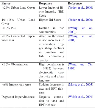
stream quality (Deacon et al.,2005). Impervious surfaces reduce the soil’s ability to infiltrate rainfall and decrease overland flow travel time to the drainage network. Using a distributed parameter runoff model, urbanized watersheds have been found to generate five times as much runoff volume and sediment yield than forested watersheds (Corbett et al.,1997). The body of literature discussing the effects of impervious surface on stream health is far too vast to cite each important peer reviewed article, however Table2.5.1neatly summarizes the area breakpoints at which urbanization causes degradation in water quality conditions.
Table 2.2: Effects of impervious surface on stream health.
Factor Response Reference
≺29% Urban Land Cover Lower Index of Bi-otic Integrity (IBI) Score
(Yoder et al.,2000)
4%≺15% Urban Land Cover
Higher IBI Score (Yoder et al.,2000)
≺10% ISC Decline in fish
communities
((Wang et al.,
2000))
≺12% Connected Imper-viousness
After this threshold minor increases in urbanization trig-ger sharp declines in baseflow and fish community quality
((Wang et al.,
2001)
≺16% Ubranization High correlation (r = 0.832) between electrolytic con-ductivity and urban land use
(Wang and Yin,
1997)
≺6% Impervious Area Sudden decrease in taxa and EPT rich-ness
(Morse et al.,2003)
Degree of Imperviousness Negative correla-tion to taxa and EPT richness
(Walsh et al.,2001)
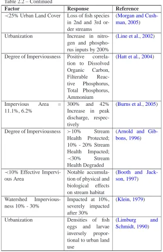
Table 2.2 – Continued
Factor Response Reference
≺25% Urban Land Cover Loss of fish species in 2nd and 3rd or-der streams
(Morgan and
Cush-man,2005)
Urbanization Increase in nitro-gen and phospho-rus inputs by 200%
(Line et al.,2002)
Degree of Imperviousness Positive correla-tion to Dissolved Organic Carbon, Filterable Reac-tive Phosphorus, Total Phosphorus, Ammonium
(Hatt et al.,2004)
Impervious Area = 11.1%, 6.2%
300% and 42% Increase in peak discharge, respec-tively
(Burns et al.,2005)
Degree of Imperviousness ≻10% Stream Health Protected; 10% - 20% Stream Health Impacted;
≺30% Stream Health Degraded
(Arnold and
Gib-bons,1996)
≺10% Effective Impervi-ous Area
Notable accumula-tion of physical and biological effects on stream habitat
(Booth and
Jack-son,1997)
Watershed Impervious-ness 10% - 30%
Impacted at 10%, severely impacted after 30%
(Klein,1979)
Urbanization Densities of fish eggs and larvae inversely propor-tional to urban land use
(Limburg and
Schmidt,1990)
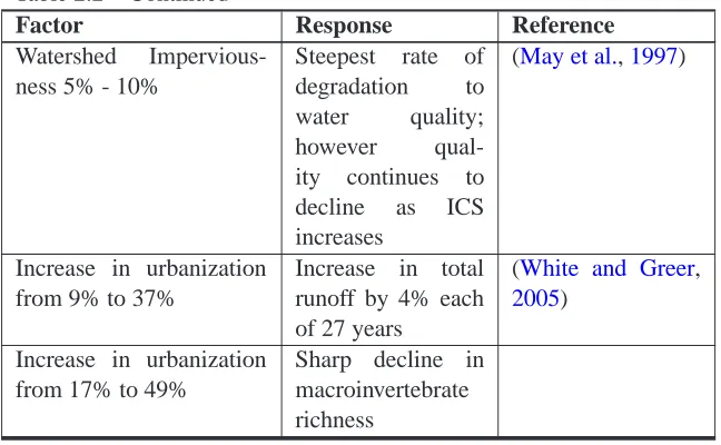
Table 2.2 – Continued
Factor Response Reference
Watershed Impervious-ness 5% - 10%
Steepest rate of degradation to water quality; however qual-ity continues to decline as ICS increases
(May et al.,1997)
Increase in urbanization from 9% to 37%
Increase in total runoff by 4% each of 27 years
(White and Greer,
2005)
Increase in urbanization from 17% to 49%
Sharp decline in macroinvertebrate richness
2.5.2 Sedimentation
A watershed in a natural state will produce sediment via sheet, rill and gully erosion
(Schiefer,2005). This combines with particles eroding from stream banks and beds to constitute
total solids load. During periods of high flow, greater amounts of sediment and larger particles are carried further downstream. During periods of high flow, sediment and particles are deposited on the substrata and form depositional features such as bars or alluvial deposits within or near the stream channel and connected floodplain.
Human impacts to the landscape such as agriculture and urbanization upset this natural balance and result in a disproportionate amount of sediment entering the stream network (Beschta
and Jackson,1979;McDonnell and Pickett,1990;Delong and Brusven,1998). It has been estimated
that depends upon the stream network maintaining its dynamic equilibrium. Sources of sediment in the stream network can be categorized as (1) channel sources originating from streambeds and banks and (2) non-channel sources originating from catchment slopes and erodible soils (Coldwell,
1957;Grimshaw and Lewin,1980).
Road networks can contribute excessive runoff during high intensity storm events leading to rapid movement of soil, sediment, and organic matter down steep stream channels (Jones et al.,
2000). Road construction has been correlated to erosion in steep landscapes (Swanson and Dryness,
1975) and the presence of a road drainage network in a catchment increases the length of the channel network and alters the erosional process (Montgomery,1994).
Burkhead and Jelks(2001) found that the decreasing rate of spawns and ripe eggs spawned
in spawning tricolor shiners (Cyprinella Trichoistia) was directly proportional to the concentration of suspended sediments within the stream channel (Lloyd et al., 1987). It has been found that excessive suspended sediment leads to a decrease in fish species requiring clean riffle pools for spawning (Sutherland et al., 2002). The same study, taking place in the Little Tennessee River Basin, North Carolina, also found that benthic crevice and gravel spawners become wiped out when a threshold of between 10 and 20% non-forested land cover is achieved, which results in a distinct increase in suspended sediment.
Excess sediment in water has been shown to effect fish species by: 1) clogging gills at lethal concentrations (Bruton,1985); 2) degrading the spawning habitat and stunting juvenile growth
(Chapman,1988); 3) modifying migratory habits of fish (Alabaster and Lloyd,1980); 4) reducing
habitat for insectivores via reduced primary production due to increased turbidity (Doeg and Koehn,
1994); and 5) affecting the ability of visual feeders to pursue prey (Ryan, 1991). Reduction of interstitial space caused by depositional sediment accumulation in headwater streams also increases the mortality rates of some salamander species (Lowe et al.,2004) and reduces the amount of refuge that adult salamanders can seek from predators. Sedimentation also has been shown to affect the quality of food consumed by snails (McIntyre et al.,2005), however this same research concluded that excess sedimentation alone is not immediately lethal to snail populations as previously stated
byArmitage and Fong(2004).
Biologic activity within the hyporheic zone within stream ecosystems is controlled by permeability of the bed substrate. Suspended sediment deposited during low flow periods intrudes porous spaces within the stream bed and degrades bed permeability. This process is referred to as colmation (Ibisch and Borchardt,2002). Silt accumulation in interstitial pores consequently reduces refugial space for invertebrates which in turn leads to a reduction in burrowing and feeding activity in streambed sediments (Hancock,2002). In a survey of interstitial only fauna, 22 taxa were found in the interstitial habitat (Mary and Marmonier,2000). It has been suggested that the lack of these taxa within the hyporheic zone, which are sensitive to elevating silt levels, indicates that degradation of water quality in the form of excess runoff is occurring upstream from the stressed habitat (Govedich et al.,1996).
Organic and inorganic particulate matter in dissolved form increases turbidity within the water present in a stream channel (Henley et al.,2000). Increased turbidity decreases the ability of light to penetrate through water and can lead to a reduction in phytoplankton production (Hoetzel
zooplankton and has a cascading effect on the entire food web (Daviescolley et al.,1992).
Poorly managed agriculture operations have been attributed to 67% of the sources of sedimentation into stream networks and this can be linked to negative impacts to stream biota (Lenat,
1984). It has been suggested in a recent study that high concentrations of suspended sediments are not lethal to some aquatic insect species, but rather the disappearance of invertebrates from impacted reaches can be attributed to the tendency of most species to avoid areas of high suspended solids or changes to the food web due to contaminant introduction to the stream network (Suren et al.,2005).
2.5.3 Nutrient Loading
Pollution entering watersheds is classified as either point or non-point sources. Point sources are generally single source locations such as sewer treatment plants, regulated mining op-erations, storm sewers outfalls, and construction sites. Non-point sources consist of the sum of all input flowing over a large land surface such as a cultivated field or an urban development, septic system leaching, atmospheric deposition, or logging activities (Carpenter et al.,1998). Non-point sources are usually the dominant sources of phosphorus and nitrogen inputs into rivers (Newman,
1995). Non-point sources of nitrogen have also been positively correlated to population density and increased by as much as 20 fold from pre-industrial times (Howarth et al.,1996). With most point sources of nutrients now subject to discharge permitting requirements, agriculture operations have been targeted as the dominant source of input of nutrients into freshwater systems (Sharpley et al.,
1994). The main cause of this non-point source is that a surplus of nutrients are often applied to agri-cultural lands, where fertilization applications far exceed production needs (Beaton et al.,1995). In a comparison of global phosphorus uptake efficiency,Isermann(1990) found that the average plant uptake efficiency in the United States was 56%, among the lowest among the nations surveyed.
Is-ermannalso found that on average, 18% of nitrogen applied as fertilizer is removed through plant
maintaining vegetated buffer strips around stream channels for the purpose of intercepting excess nutrients is highlighted by Osborne and Kovacic(1993), who, in a review of 21 vegetated buffer strip studies, found that buffers of 0-50 m in width removed 40 - 100% of nitrate and phosphorus applied upslope of the riparian buffers.
In urbanized catchments, N loading can be 45% higher than that of a forested catchment
(Wollheim et al.,2005). Some studies suggest that highly-urbanized catchments (greater than 35%
impervious surface) in the Neuse River Basin contribute more N to streams than do predominantly agricultural catchments (Lunetta et al.,2005). Seven percent of the Neuse River Basin is covered with managed turf grass (Osmond and Hardy, 2004). Osmond and Hardy(2004) illustrated some rather surprising trends regarding N sources to the Neuse River:
• Cary, NC had the smallest average turf area per household yet had the highest rate of lawn care service use.
• Lawn care services applied on average 50 kg/ha more fertilizer than homeowner self applica-tion.
• Cary residents had the lowest average of removing fertilizer pellets from impervious surfaces after application.
• Two times as much fertilizer is applied to crops in the Neuse Basin as is applied to all of the turf grass in the entire state.
issue in coastal estuaries (NRC,1993). The National Research Council (NRC) has also published findings that trace sources of contamination to agriculture operations, development, acid rain, strip mining, and invasive species (NRC,1992). Eutrophication leads to algae blooms which consume oxygen as they decompose and lead to anoxic conditions (Anderson, 1997). These blooms poison shellfish rendering them harmful to human consumption and have been linked to increased mortality rates in marine species off the Atlantic coast (Anderson, 1997;Burkholder et al.,1992). Nitrogen inputs to headwaters in the Neuse River basin in North Carolina have been shown to increase phy-toplankton biomass and a correlated increase in pfiesteria zoospores which has been directly linked to algal blooms and fish kills in the Neuse River Estuary (Pickney et al., 1998). Increased phy-toplankton biomass decreases light penetration thus reducing the ability of photosynthetic oxygen production to balance oxygen consumption (Meyercordt and Meyer-Reil,1999). Small changes in this penetration depth have catastrophic consequences on aquatic communities in shallow estuaries such as the Neuse River (Fear et al.,2004).
2.6
Stream Management Regulatory Programs
2.6.1 Federal Regulation
2.6.2 North Carolina Regulation
2.7
References Cited
Alabaster, J. S., Lloyd, R., 1980. Water quality criteria for freshwater fish. Butterworths, London.
Allan, J. D., Erickson, D. L., Fay, J., 1997. The influence of catchment land use on stream integrity across multiple spatial scales. Freshwater Biology 37 (1), 149–161.
Anderson, D. M., 1997. Bloom dynamics of toxic alexandrium species in the northeastern US. Limnology And Oceanography 42 (5), 1009–1022.
Armitage, A. R., Fong, P., 2004. Upward cascading effects of nutrients: shifts in a benthic microal-gal community and a negative herbivore response. Oecologia 139 (4), 560–567.
Arnold, C. L., Gibbons, C. J., 1996. Impervious surface coverage - the emergence of a key environ-mental indicator. Journal Of The American Planning Association 62 (2), 243–258.
Beaton, J. D., Roberts, T. L., Halstead, E. H., Cowell, L. E., 1995. Global transfers of P in fer-tilizer materials and agricultural communities. In: Tiessen, H. (Ed.), Phosphorus in the global environment: transfers, cycles and management. Wiley, Chichester; New York, pp. 7–26.
Bent, G. C., Archfield, S. A., 2002. A logistic regression equation for estimating the probability of a stream flowing perennially in Massachusetts. Water-Resources Investigations Report 02-4043, U.S. Geological Survey.
Beschta, R. L., Jackson, W. L., 1979. Intrusion of fine sediments into a stable gravel bed. Journal Of The Fisheries Research Board Of Canada 36 (2), 204–210.
Booth, D. B., Jackson, C. R., 1997. Urbanization of aquatic systems: Degradation thresholds, stormwater detection, and the limits of mitigation. Journal Of The American Water Resources Association 33 (5), 1077–1090.
Brunke, M., Gonser, T., 1997. The ecological significance of exchange processes between rivers and groundwater. Freshwater Biology 37 (1), 1–33.
Bruton, M. N., 1985. The effects of suspensoids on fish. Hydrobiologia 125 (JUN), 221–241.
Burkhead, N. M., Jelks, H. L., 2001. Effects of Suspended Sediment on the Reproductive Success of the Tricolor Shiner, a Crevice-Spawning Minnow. Transactions of the American Fisheries Society 130 (5), 959–968.
Burkholder, J. M., Noga, E. J., Hobbs, C. H., Glasgow, H. B., 1992. New phantom dinoflagellate is the causative agent of major estuarine fish kills. Nature 358 (6385), 407–410.
Burns, D., Vitvar, T., McDonnell, J., Hassett, J., Duncan, J., Kendall, C., 2005. Effects of subur-ban development on runoff generation in the Croton River Basin, New York, USA. Journal of Hydrology 311 (1-4), 266–281.
Carpenter, S. R., Caraco, N. F., Correll, D. L., Howarth, R. W., Sharpley, A. N., Smith, V. H., 1998. Nonpoint pollution of surface waters with phosphorus and nitrogen. Ecological Applica-tions 8 (3), 559–568.
Chapman, D. W., 1988. Critical-review of variables used to define effects of fines in redds of large salmonids. Transactions Of The American Fisheries Society 117 (1), 1–21.
Corbett, C. W., Wahl, M., Porter, D. E., Edwards, D., Moise, C., 1997. Nonpoint source runoff modeling - a comparison of a forested watershed and an urban watershed on the South Carolina coast. Journal of Experimental Marine Biology and Ecology 213 (1), 133–149.
Correll, D. L., Weller, D. E., 1989. Factors limiting processes in freshwater wetlands: An agricul-tural primary stream riparian forest. In: Sharitz, R., W., G. J. (Eds.), Freshwater Wetlands and Wildlife. United States Department of Energy, Oak Ridge, Tenn, pp. 9–23.
Daily, G. C., 1997. Nature’s services: societal dependence on natural ecosystems. Island Press, Washington, DC.
Daviescolley, R. J., Hickey, C. W., Quinn, J. M., Ryan, P. A., 1992. Effects of clay discharges on streams.1: Optical-properties and epilithon. Hydrobiologia 248 (3), 215–234.
Deacon, J. R., Soule, S. A., Smith, T. E., 2005. Effects of urbanization on stream quality at selected sites in the seacoast region in New Hampshire, 2001-03. Scientific Investigations Report 2005-5103, U.S. Geological Survey.
Delong, M. D., Brusven, M. A., 1998. Macroinvertebrate community structure along the longitudi-nal gradient of an agriculturally impacted stream. Environmental Management 22 (3), 445–457.
Dietrich, W., Reneau, S., Reneau, C., 1987. Overview: ’zero-order basins’ and problems of drainage density, sediment transport and hillslope morphology. In: Erosion and Sedimentation in the Pa-cific Rim. International Association of Hydrological Sciences, Corvallis, Or, pp. 27–37.
Dietrich, W. E., Dunne, T., 1993. The channel head. In: Beven, K., Kirkby, M. J. (Eds.), Channel Network Hydrology. John Wiley, New York, pp. 175–219.
Department of Public Works and Environmental Services (DPWES), 2006. Perennial Stream Clas-sification Protocol [Online]. Fairfax County, Virginia. Available at http://www.fairfaxcounty.gov/
dpwes/watersheds/ps protocols.pdf. Accessed 10 June 2006.
Dunne, T., Leopold, L. B., 1978. Water in environmental planning. W. H. Freeman, San Francisco.
Fear, J., Gallo, T., Hall, N., Loftin, J., Paerl, H., 2004. Predicting benthic microalgal oxygen and nutrient flux responses to a nutrient reduction management strategy for the eutrophic Neuse River Estuary, North Carolina, USA. Estuarine, Coastal and Shelf Science 61 (3), 491–506.
Ferguson, B. K., 1994. The concept of landscape health. Journal of Environmental Management 40 (2), 129–137.
Fisher, S. G., Likens, G. E., 1973. Energy flow in Bear Brook, New Hampshire - integrative ap-proach to stream ecosystem metabolism. Ecological Monographs 43 (4), 421–439.
Foster, G. R., 1986. Understanding ephemeral gully erosion. In: Assessing the National Research Inventory. National Academy Press, Washington, D.C., pp. 90–125
Govedich, F., Oberlin, G., Blinn, D. W., 1996. Comparison of channel and hyporheic invertebrate communities in a Southwestern USA desert stream. Journal Of Freshwater Ecology 11 (2), 201– 209.
Gregory, S. V., Swanson, F. J., Mckee, W. A., Cummins, K. W., 1991. An ecosystem perspective of riparian zones. Bioscience 41 (8), 540–551.
Grimshaw, D. L., Lewin, J., 1980. Source identification for suspended sediments. Journal Of Hy-drology 47 (1-2), 151–162.
habitats - implications for management. Aquatic Conservation-Marine And Freshwater Ecosys-tems 5 (2), 143–166.
Guy, H. P., 1970. Fluvial sediment concepts. In: Techniques of Water-Resources Investigations of the United States Geological Survey, Book 3, Chapter C1. U.S. Geological Survey.
Hack, J., 1975. Dynamic equilibrium and landscape evolution,. In: Melhorn, W.N. and Flemal, R.C. (Eds.), Sixth Annual Binghampton Symposium. Theories of Landform Development, Proceed-ings of the Sixth Annual Binghampton Symposium. pp. 87–102.
Hancock, P. J., 2002. Human impacts on the stream-groundwater exchange zone. Environmental Management 29 (6), 763–781.
Hansen, W. F., 2001. Identifying stream types and management implications. Forest Ecology and Management 143 (1-3), 39–46.
Harman, W. A., Jennings, G. D., 1999. River course: Natural stream processes [Online]. North Carolina Cooperative Extension Service. Available at http://www5.bae.ncsu.edu/programs/
extension/wqg/sri/rv-crs-1.pdf. Accessed 12 August 2006.
Harner, M. J., Ramsey, P. W., Rillig, M. C., 2004. Protein accumulation and distribution in flood-plain soils and river foam. Ecology Letters 7 (9), 829–836.
Hatt, B. E., Fletcher, T. D., Walsh, C. J., Taylor, S. L., 2004. The influence of urban density and drainage infrastructure on the concentrations and loads of pollutants in small streams. Environ-mental Management 34 (1), 112–124.
Hedman, E. R., Osterkamp, W. R., 1982 Streamflow characteristics related to channel geometry of streams in Western United States, Water Resources Investigations Report 82-4092, U.S. Geolog-ical Survey.
Henley, W., Patterson, M., Neves, R., Lemly, A., 2000. Effects of sedimentation and turbidity on lotic food webs: A concise review for natural resource managers. Reviews in Fisheries Science 8 (2), 125–139.
Hetrick, N. J., Brusven, M. A., Meehan, W. R., Bjornn, T. C., 1998. Changes in solar input, water temperature, periphyton accumulation, and allochthonous input and storage after canopy removal along two small salmon streams in Southeast Alaska. Transactions Of The American Fisheries Society 127 (6), 859–875.
Hewlett, J. D., 1982. Principles of forest hydrology. University of Georgia Press, Athens, Ga.
Hewlett, J. D., Hibbet, A. R., 1967. Factors affecting the response of small watersheds to precipita-tion in humid areas. In: 1st Internaprecipita-tional Symposium on Forest Hydrology. pp. 253–275.
Hickin, E. J., 1984. Vegetation and river channel dynamics. Canadian Geographer-Geographe Cana-dien 28 (2), 111–126.
Hoetzel, G., Croome, R., 1994. Long-term phytoplankton monitoring of the Darling River at Bur-tundy, New South Wales: Incidence and significance of cyanobacterial blooms. Australian Jour-nal of Marine and Freshwater Research 45 (5), 747–759.
Horton, R. E., 1945. Erosional development of streams and their drainage basins - hydrophysical approach to quantitative morphology. Geological Society Of America Bulletin 56 (3), 275–370.
Z. L., 1996. Regional nitrogen budgets and riverine N&P fluxes for the drainages to the North Atlantic Ocean: Natural and human influences. Biogeochemistry 35 (1), 75–139.
Hursh, C. R., 1936. Storm-water and absorption. Transactions of the American Geophysical Union 17 (2), 301–302.
Ibisch, R., Borchardt, D., 2002. Influences of periphyton biomass dynamics on biological colma-tion processes of the hyporheic zone. Proceedings of the North American Benthological Society Annual meeting. Pittsburgh, PA.
Isermann, K., 1990. Share of agriculture in nitrogen and phosphorus emissions into the surface waters of Western-Europe against the background of their eutrophication. Fertilizer Research 26 (1-3), 253–269.
Istanbulluoglu, E., Tarboton, D., Pack, R., 2002. A probalistic approach for channel initiation. Water Resources Research 38 (12), 61(1)–61(14).
Jones, J. A., Swanson, F. J., Wemple, B. C., Snyder, K. U., 2000. Effects of roads on hydrology, geomorphology, and disturbance patches in stream networks. Conservation Biology 14 (1), 76– 85.
Karr, J. R., 1981. Assessment of biotic integrity using fish communities. Fisheries 6 (6), 21–27.
Kawaguchi, Y., Nakano, S., 2001. Contribution of terrestrial invertebrates to the annual resource budget for salmonids in forest and grassland reaches of a headwater stream. Freshwater Biology 46 (3), 303–316.
Klein, R. D., 1979. Urbanization and stream quality impairment. Water Resources Bulletin 15 (4), 948–963.
Lenat, D. R., 1984. Agriculture and stream water-quality - a biological evaluation of erosion control practices. Environmental Management 8 (4), 333–343.
Limburg, K. E., Schmidt, R. E., 1990. Patterns of fish spawning in Hudson River tributaries - re-sponse to an urban gradient. Ecology 71 (4), 1238–1245.
Lindenmayer, D., Franklin, J. F., 2002. Conserving forest biodiversity: a comprehensive multiscaled approach. Island Press, Washington, DC.
Line, D. E., White, N. M., Osmond, D. L., Jennings, G. D., Mojonnier, C. B., 2002. Pollutant export from various land uses in the upper Neuse River Basin. Water Environment Research 74 (1), 100– 108.
Lloyd, D., Koenings, J. P., Laperriere, J. D., 1987. Effects of turbidity in freshwaters of Alaska. North American, Journal of Fisheries Management 7, 18–33.
Lowe, W. H., Nislow, K. H., Bolger, D. T., 2004. Stage-specific and interactive effects of sedimen-tation and trout on a headwater stream salamander. Ecological Applications 14 (1), 164–172.
Lowrance, R., Leonard, R., Sheridan, J., 1985. Managing riparian ecosystems to control nonpoint pollution. Journal of Soil and Water Conservation 40 (1), 87–91.
Lunetta, R. S., Greene, R. G., Lyon, J. G., 2005. Modeling the distribution of diffuse nitrogen sources and sinks in the Neuse River Basin of North Carolina, USA. Journal Of The American Water Resources Association 41 (5), 1129–1147.
May, C., Horner, R., Karr, J., Mar, B., Welch, E., 1997. Effects of urbanization on small streams in the Puget Sound Lowland Ecoregion. Watershed Protection Techniques 2, 483–494.
McDonnell, M. J., Pickett, S. T. A., 1990. Ecosystem structure and function along urban rural gradients - an unexploited opportunity for ecology. Ecology 71 (4), 1232–1237.
McIntyre, P. B., Michel, E., France, K., Rivers, A., Hakizimana, P., Cohen, A. S., 2005. Individual-and assemblage-level effects of anthropogenic sedimentation on snails in Lake Tanganyika. Con-servation Biology 19 (1), 171–181.
Meyer, J. L., Wallace, J. B., 2001. Lost linkages and lotic ecology: Rediscovering small streams. In: Press, M. C., Huntly, N. J. (Eds.), Ecology: Achievement and Challenge. Blackwell Scientific Publications, Oxford, MA, pp. 295–317.
Meyercordt, J., Meyer-Reil, L. A., 1999. Primary production of benthic microalgae in two shallow coastal lagoons of different trophic status in the Southern Baltic Sea. Marine Ecology Progress Series 178, 179–191.
Montgomery, D., Foufoula-Georgiou, E., 1993. Channel network source representaion using digital elevation models. Water Resources Research 29 (12), 3925–3934.
Montgomery, D. R., 1994. Road surface drainage, channel initiation, and slope instability. Water Resources Research 30 (6), 1925–1932.
Moore, I. D., Larson, C. L., 1979. Estimating microrelief surface storage from point data. Transac-tion of the American Society of Agricultural Engineers 20, 1073–177.