Strategy for scalable scenarios modeling and calculation in early software reliability engineering

77:9 (2015) 139–148 | www.jurnalteknologi.utm.my | eISSN 2180–3722 |

Jurnal

Teknologi

Full Paper

S

TRATEGY FOR

S

CALABLE

S

CENARIOS

M

ODELING AND

C

ALCULATION

IN

E

ARLY

S

OFTWARE

R

ELIABILITY

E

NGINEERING

Awad Ali

_{, Dayang N. A. Jawawi}

_{, Mohd Adham Isa}

a

_{Department of Software Engineering, UTM, Johor, Malaysia}

_{University of Kassala, Kassala, Sudan}

Article history

Received

2 February 2015

Received in revised form

8 October 2015

Accepted

12 October 2015

*Corresponding author

[email protected]

Graphical abstract

Abstract

System scenarios derived from requirements specification play an important role in the early software reliability engineering. A great deal of research effort has been devoted to predict reliability of a system at early design stages. The existing approaches are unable to handle scalability and calculation of scenarios reliability for large systems. This paper proposes modeling of scenarios in a scalable way by using a scenario language that describes system scenarios in a compact and concise manner which can results in a reduced number of scenarios. Furthermore, it proposes a calculation strategy to achieve better traceability of scenarios, and avoid computational complexity. The scenarios are pragmatically modeled and translated to finite state machines, where each state machine represents the behaviour of component instance within the scenario. The probability of failure of each component exhibited in the scenario is calculated separately based on the finite state machines. Finally, the reliability of the whole scenario is calculated based on the components’ behaviour models and their failure information using modified mathematical formula. In this paper, an example related to a case study of an automated railcar system is used to verify and validate the proposed strategy for scalability of system modeling.

Keywords: Reliability engineering, architecture-based reliability, scenario-based reliability, component-scenario-based software, software quality

Abstrak

mengesahkan strategi yang dicadangkan untuk penskalaan permodelan system.

Kata kunci: Kebolehpercayaan kejuruteraan, kebolehpercayaan berasaskan senibina, kebolehpercayaan berasaskan scenario, perisian berasaskan komponen, kualiti perisian

© 2015 Penerbit UTM Press. All rights reserved

1.0 INTRODUCTION

Failure of software can lead to critical events and fatal consequences in safety-critical applications as well as in business applications. In order to meet customer expectations and needs, the software must have high

reliability. Increasing demands on software

functionalities are leading to various issues, which include the scalability and degree of concurrency of the software system. Customer satisfaction is also a serious challenge; thus software reliability engineering should live up to today’s complex software systems and their specific challenges.

The reliability approach is formalized to explain the failure behaviour within the system. Software reliability is defined as the probability that the software system will perform a required function correctly (failure free) in a stated environment for a specified period of time [1, 2]. Due to the heterogeneity of the execution environment and the development methodology of the current software systems, a failure broadly can mean that the software system is unable to deliver the expected service and is not capable of resuming its service as it was not interrupted. Several kinds of failures are possible during service execution, such as faults in the implementation of the software components, hardware failure and network failure. Hardware failure is due to an unreliable hardware resource, and network failure is just because the message is lost or there is a problem in inter-component communication [3, 4]. Predicting software reliability at design-time enables the software designer to identify weak design spots, which would be more cost-effective to improve than fixing consequent errors at later implementation phases. Therefore, the reliability approach must be able to work at the early design stage, and particularly during the architectural design.

During the last decade, researchers have proposed many approaches to predict reliability depending upon architectural design and targeting design-time specification. These approaches address different problems and challenges. However, extension of a scenario specification toward partial behaviour modeling is integral part that should be considered to predict the reliability based on the architecture [5, 6]. Except for certain approach [7], which we will discuss in the related work, most of the current approaches [8-17] compute the reliability based upon large behavioural models, without taking into account the

scalability problem (e.g., dealing with applications consist of a large number of components).

To address the problem of scalability, a partial behaviour modeling approach is presented in this paper using expressive scenario specification language and finite state machine. The scenario language describes system scenarios in a compact and concise manner that enables the system engineer to model the system in fewer scenarios. The finite state machine explains the basic states of the scenario and helps in computation along limited space so as to avoid the computational complexity.

The rest of the paper is divided into six sections. Section 2 describes the research background. Section 3 describes in brief the proposed strategy. The details of behaviour modeling are given in Sections 4. The reliability calculation strategy is given in Section 5. Furthermore, Section 6 is about related work and it compares and classifies the current works based on the proposed strategy. Section 7 concludes the research and identifies future research directions.

2.0 BACKGROUND

This section briefly defines and reviews the concepts of system scenarios and behaviour models, on which we base our modeling and calculation of system scenarios. The running example that used to illustrate the different proposed aspects is also introduced. Finally, an outline is given which illustrates the proposed strategy.

2.1 System Scenarios and Behaviour Models

Two common ways for describing and documenting system requirements specification have been found very useful in practice, particularly at earlier stages of system design. One is scenarios based that describes how the different components in the system interact, for example, UML sequence diagrams (SD), and Message Sequence Charts (MSC) [18]. The other way is state description language that describes and defines conditions and constraints among the internal states of individual components, for example, Object Constraint Language (OCL) [19], and VDM Specification Language (VDM-SL) [20].

MSC by adding liveness. LSC equipped to describe alternative and repetitive behaviour, synchronous, asynchronous, data values on messages, and symbolic instances. In addition, there are characteristics that enable making explicit causality relations between different behaviours by means of conditional, triggered and pre-empted behaviour. LSC describes system scenarios in two types of charts: an existential live sequence charts (eLSC) and a universal sequence charts (uLSC). eLSC are more like MSC and SD [22]. The eLSC scenarios define an example of system behaviour, and must be satisfied through at least one system run. The uLSC scenarios describe a rule that all system behaviour is expected to satisfy; they encapsulate a conditional behaviour as action and reaction, using a pre-chart and main chart: once the pre-chart occurs, the main chart must occur. The reason being that during the requirements obtained from the domain knowledge, there is a progressive movement from existential statements, in the formula of examples and use-cases to universal statements in the formula of declarative properties. Most important point of uLSC scenarios, they document the last confirmation of the system requirements specification. Thus, behaviour models generated from them are more accurate than the behaviour models build from other charts.

In this research work, the system requirements specification is described by extended uLSC charts and OCL. The extended uLSC is part of this paper’s contribution (defined in section 4.1). Then these specifications are translated to a set of finite state machines (FSM). FSM are simply directed graphs, with nodes denoting states, and arrows (labelled with the triggering events and guarding conditions) denoting transitions [23]. FSM describes the dynamic behaviour of system in a sequential flow. Most of behaviour modeling approaches converts FSMs to other type of state representation graphs such as statecharts [23], Labeled Transition System (LTS) [24], and Modal Transition System (MTS)[25], in order to expressively allow for more compact representation of large and complex software systems. However, in this research work, calculation of reliability was built upon the basic behaviour models without the need of integration to complex behaviour models.

2.2 Running Example

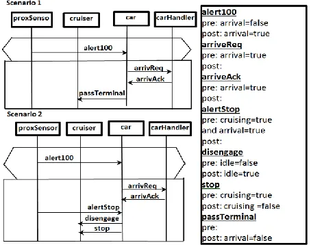
An ongoing example is used in this paper to illustrate the proposed strategy. The automated railcar system presented in [26], and already used in our previous work [27] is selected as the ongoing example. Because our main goal is to improve our previous work by achieving more scalability via reducing number of scenarios, thus, use of this example can ease the comparison. The railcar system consists of six terminals located on a cyclic path, and each pair of adjacent terminals is linked by two rail tracks. Many railcars are existed to carriage passengers between terminals. A number of scenarios have been depicted in the previous work [27], for ease of illustration, in this paper

our focusing will be on two of them: scenario of car approaching to the terminal with stopping at that terminal (scenario 1 in Figure 1), and scenario of car approaching to the terminal with passing the terminal (scenario 2 in Figure 1). The scenarios consisted of four components named: proxSensor, cruiser, car, and carHandler. The details of the scenarios are depicted in Figure 1.

Figure 1 Portion of Railcar system specifications

3.0 THE PROPOSED STRATEGY

The proposed strategy has four steps as detailed below. These steps are distributed into two phases, behaviour modeling (Section 4.0) and reliability calculation (Section 5.0).

 Describing of system scenarios using extended uLSC notations.

 Annotation of scenario specification using system constraints

 Translation of annotated scenarios to FSMs.

 Determination of components’ criticalities.

 Calculation of scenarios reliability.

(components interactions), in turn, avoiding the state space explosion problem. Figure 2 depicts the strategy phases and steps.

Figure 2 The proposed strategy phases and steps

Modeling phase focuses on moving from scenario-based specification to state scenario-based specification. Unlike most of reliability approaches, in the modeling we move from system specification explicitly. Most approaches rely on Markov notations directly (state based specification) as a primary modeling notation without describing how the states generated. In the calculation phase, the calculation conducts partially. Given the state specification of the scenarios, the calculation adopts mathematical formula to tackle the state space partially. The following sections describe the phases in details.

4.0 BEHAVIOUR MODELING

By documenting the behaviour of the system in two different and complementary ways of requirements specification (as scenarios notations (e.g. uLSC) and constraints (e.g. OCL)), the architects of the system are forced to truly understand the requirements specification and the behaviour implied by them. In Figure 1, the requirements specifications are documented by uLSC. As mentioned before, the characteristic of uLSC compared to eLSC and other scenario notations, they give the last confirmation of the requirements specification. Unfortunately, use of uLSC as single scenarios notation produces increase number of scenarios (each action and its reaction documented separately). In case of large software systems there is need for a scenario language that can reduce the number of the scenarios. Thus, the uLSC

notations are extended to hold more than one scenario specifications, by adopting constructs from UML 2.0 SD[28].

4.1 Moving from uLSC to Extended uLSC

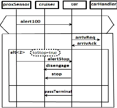
In the scenario description, an extended form of uLSC is used, which includes additional constructs. Part of these constructs is adopted from UML 2.0 SD such as interaction combined fragment with alt operator. The idea was to constructs an uLSC that is able to combine more than one uLSC bases on the similarity between triggers. After unifying the pre-chart of scenarios, the main charts are combined via a combined fragment notation with alt operator. A combined fragment is expression of an interaction by a box contains a subset of messages and is defined by an operator (e.g. alt), which states the connection between the fragment's messages. An alt is an operator which denotes that the messages within the fragment are alternatives to each other. Each alternative has a guard and contains the interaction that occurs when the condition for that guard is met. Only one of the conditions can occur at the same time. An 'alt' combined fragment is similar to nested if-then-else and switch/case constructs in programming languages. Conditions in the guards can be described as implied triggers. Figure 3 depicts the extension idea by drawing a single uLSC holding scenario 1 and scenario 2 of the running example.

Figure 3 The extended uLSC combing scenario 1 and scenario 2 of railcar system

4.2 Annotate the Scenario Specification by System Constraints

constraints and their state variables as basic information sources to depict the component's behavior precisely. The constraints and their state variables (called as a set, state vector) are already provided as domain knowledge related to early design specification. For example, the state vector of the railcar system based on the constraints shown in Figure 1 is: < “idle, cruising, arrival”>.

Component state vector is a vector holding a state variable(s) elicited from the system state vector and its values represent the component state before and after each operation (message). The component state vector is employed in the strategy to annotate the scenario specification based on the system constraints. The following steps give details of how component state vector elicited and then how it can be employed to annotate the scenario specifications.

i) Elicit component’s state vector:

Component state vector uses as pre- and post-conditions to component’s operations invocation (incoming and outgoing messages). Therefore, in order to elicit component state vector, following procedures are needed. Firstly, the determination of component’s incoming and outgoing messages. Secondly, the addition of each state variable appears in the preconditions of the outgoing messages to component’s state vector. Finally, the addition of each state variable modified by the component’s incoming or outgoing messages to the component’s state vector. The previous procedures can be defined formally as follows:

Definition 1: (Sets of component’s incoming and outgoing messages):

Let compom and compim be the sets of outgoing and

incoming message of the component i (compi)

respectively. compi extended uLSC , a message

mi  extended uLSC will be added to the compom iff

mi sent by the compi to other components within the

extended uLSC; and mi will be added to the compim iff

it was received by compi from other components

within the extended uLSC.

Definition 2: (State vector and pre-conditions):

Let compsv be a component’s state vector.





compom if





constraints, then the state variable that appear in the preconds of the opname will be added to the compsv iff is

not already existing in compsv.

Definition 3: (state vector and the modified variables):











opname does not matching the value of postconds, then

the state variables related to the preconds or postconds

will be added to the compsv iff does not already

existed in compsv.

For example, according to these definitions and the railcar constraints, the state vector of the car component is < idle, cruising, arrival >, cruiser: < idle,

cruising>, the proxSensor: < cruising, arrival >, and the carHandler component is: < arrival >.

ii) Scenario annotation and propagation:

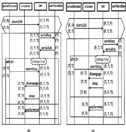
After the elicitation of the state vector of each component, annotation and propagation of the component’s within the scenario can be conducted similar to the techniques in [29] and [30]. The goal of the annotation procedure is to enrich component information by defining the system state from a component’s perspective before and after execution of each operation depicted in the scenario. In this procedure, firstly, annotation parameters are built based on variables of the state vector and their values in the system constraints (e.g. see Figure 4 below). The annotation values before and after each operation is determined according to the system constraints. Some operations (messages) may not be given a specification specifying system state before or after; so, secondly, the propagation process is used to propagate unknown values (?) in (before and after) the annotations. Propagation is executed using the technique in [29]. Figure 4(a) shows annotation result of our running example and Figure 4(b) shows the annotation result after the propagation.

Figure 4 (a) Annotation result of railcar example (b) The annotation after propagation

3.3 Translate the Annotated Scenario to FSMs

(S,S ,S ,T)₀

i

Fm b be a FSM synthesized from instance i in

m. The basic idea is to construct a state for each state vector value. Thus, S is the set of states corresponding to the state vector values along the instance. S0

contains exactly the state corresponding to the first state vector value. Sb contains state corresponding to

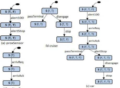
the branching state vector value if it existed (first state vector value in the combined fragment box). T is a transition relation labelled with associated messages sent or received by the instance. Figure 5, shows FSMs for railcar system components translated from the scenario in Figure 4.

Figure 5 The obtained FSMs of the railcar system components

5.0 RELIABILITY CALCULATION

Once the FSMs of the scenario are given, scenario’s reliability can be calculated. The calculation builds upon mathematical formula tackling each FSM separately to avoid the computation complexity. The following sub sections defines calculation formulas and discusses calculation results.

5.1 Calculation Formulas and Failure Information

Let comp1, comp2,…, compK denote the K

components participated in scenario Scj . Let fi be the

failure probability of the component compi and assume fi’s to be known. Let ni be the number of invocation of component i within the scenario Scj. Recall that fij is the probability that the ith component

(compi) fails in the jth _{scenario (Scj). The value of fij can} be computed by [31]:

1 (1

)

ij i

f

  

f

From Equation (1), assuming that component failure probabilities are independent, the scenario failure probability

_{fSc j}

1

1

(1

)

j

K

n

Sc i

i

f

f



 





Design specifications depicted by our scenario description notation can reveal both structural and behavioural inconsistencies among component interaction. However, identification and classification of these inconsistences are beyond the scope of this paper. In particular, they reveal directional errors as well as mismatches among interface signatures and pre- and post-conditions, more details about such type of errors can be found in [32]. However, all these errors are related to components required and provided services which implemented via component operations, thus, all these types of errors are abstracted and encapsulated in operations’ failure probability. In the previous work [27], the failure probability of the whole component is used as failure information required as an input for equation (2) in order to calculate reliability of scenario. In this paper, to be more accurate, the failure probability of operations will be used as alternatives to component failure. This use due to the fact that component failure estimates or calculates as a function of the entire component states, while in each interaction moment, only specific set of operations participates in the failure.

By observing to the scenario descriptions, for example, the operations that a component executes at each specific time can be identified exactly. Following this line of thinking, _fi can be replaced with a set of operation failure probabilities l

f i, where ,...,

1

l l _ln is the index of the operation within the

component. Equation (1), in this case, becomes:

1

1

(1

)

n

l

l

ij i

l l

f

f



 





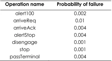
Failure information needed now is the probabilities of failure of the operation such as the information shown in Table 1 which is related to the operations invoked in the railcar system. As mentioned previously, the failure information will be tackled abstractly, therefore, this paper’s illustration is not limited to specific type of error, a preliminary estimate of l

Table 1 Failure information of each operation in the railcar scenario

Operation name Probability of failure alert100 0.002 arriveReq 0.01 arriveAck 0.004 alertStop 0.004 disengage 0.001

stop 0.001

passTerminal 0.004

From Equation (3), assuming that component failure probabilities are independent, the scenario failure probability

_{fSc j}

equation (3); thus

_{fSc j}

1

1

1

(1

)

n

j

l K

l

Sc i

i l l

f

f

 

 





Note that equation (3) and (4) are only feasible under the assumptions that: an operation’s failure probability does not depend on the failure probabilities of other operations and the scenario is a

sequential structure. Unfortunately, important

enhancement made by extend uLSC is the propose of branching notation, this in the most cases will produce branching scenarios (e.g. see FSMs of car and cruiser components in Figure 4); thus, for more accurate, in case of branching scenario, for equation (3) and (4) the calculation can be done by considering each branch as a sequential structure, and then taking the mean of the branches before the subtraction from 1.

The scenario reliability can be defined as the probability of not being in a failure state; thus reliability of scenario Scj is computed as:

1

Scj Scj

R

 

f

5.2 Results of Calculation and Discussion

Once FSMs of the scenario have been derived from the extended uLSC where, each FSM represents a component instance, the next step is to calculate the reliability of the scenario. Using Equation (3) and values of the expected failure of the operations invoked by the component, the probability of component failure is calculated. By calling back our railcar system the probabilities of failure of the components proxSensor, cruiser, car, and carHandler are: 0.0059920, 0.002995, 0.0208480, and 0.0139600 respectively. These values denote to the criticality of these components regarding to the scenario and then the system. Applying Equation (4), if the branching structure of the components is not considered, the probability of failure of the whole scenario will be 0.050818. Based on this failure probability and using

Equation (5), the reliability of the scenario is 0.949182. By considering the branching structure of cruiser and car components (taking mean of branches failure) probability of failure of the scenario will be 0.047004 and thus reliability of the scenario is 0.952996. The difference between the reliability values in the case of considering versus ignoring the branching structure is 0.003814. This difference in some applications, may seems relatively small, however, in the case of long branches, the difference can be significant. Thus, considering the weighted mean value would be deemed helpful. Furthermore, a weighted mean that takes into account the number of states in the branches represent a more accurate model of the actual system.

Summing up, the scenario reliabilities calculation based on the system requirements specifications have been discussed. These specifications were modeled through a scalable scenario description (the scenario modeled in a compact and concise manner). After the scenarios calculation stage, the system global behaviour model can be constructed in hierarchical (e.g. see [7]) or flat (e.g. see [24]). In the global behaviour model of the system, the scenarios can represent the basic elements as alternative to the components potentially reducing the complexity of the system global structure (e.g. a software system may consist hundreds of components). Each scenario will represent node in the structure. The relation and connections among these nodes (scenarios) will be determined based on the information of the system specification (e.g. eLSCs and system documents) and operational profile artifact, which can describe the related and unrelated behaviours. After global model construction, reliability of the system can be computed using any reliability technique [10, 35] or formula [13, 36] that provided to utilize system structures and behaviour in the prediction.

6.0 RELATED WORK

During the last decade, researchers proposed several approaches to predict reliability at the design-time utilizing the architectural design of the software system and the interaction scenarios of components; these

approaches address different problems and

challenges. For the sake of brevity, a brief overview of the approaches of greatest interest to the scope of this paper’s work is provided. The approaches classified to two groups, bases on their closeness to this paper’s work.

states. The architecture analysis is used based on Quartert views to reveal the potential problems of design and implementation. Result of architecture analysis are built based on Quartert views of this work and can be used as input to the proposed strategy in this paper. However, in the work [37] and [24] the total behaviour of system is represented by a flat model. The flat model as reported in [7] suffers from scalability problem. The main reason for these problems is the number of states which is also known as state explosion problem, exactly, in the case of large systems. Authors of [7] proposed extension to the work in [37] by modeling and calculating system scenarios hierarchically. The hierarchical method can provide solution in the case of large systems, especially when

the synchronization nature of the system

implementation is taken into account [6]. However language of scenario description is message sequence charts in classical form. Thus, the description of system scenarios in a compact and concise manner toward archiving scalability is not addressed by the approaches in [7] and even in[38]. Moreover, there is no new calculation strategies that consider computation complexity are presented in most of these approaches.

In the second group the approaches [3, 4] address the utilization of usage profiles and the component environment, to predict the system reliability in the deployment environment of the system. In [4] the previous usage information which is named as architectural kens and defined as a parameters store the error probability of component, while there are no specifications about how the values are obtained. The work in [3] extends the ideas in [4] by utilizing the usage profiles. Furthermore, this approach includes hardware factor (failures caused by communication links or hardware) in the reliability calculation. The usage-profile is built upon parameter dependencies. The parameters dependencies concept is about the influence of the input values on the control and data flow. These values are derived from the usage scenarios by domain expert and treated as a stochastic expression and the probability distribution of the failure. However, unlike our proposed work, these approaches focus on the structural aspects rather than the behavioural aspects of the component interactions.

Comparatively, our work enhances the work of the first group, that is, by adding more scalability by using extended scenario description language that describes the system scenarios in a compact and concise manner. Furthermore, our work provides promising scenario calculation strategy, treated the calculation partially. In fact, unlike most of the first group approaches (i.e. lack of step-by-step

traceability), our strategy forces traceable mapping from system specification to the reliability calculation through explicitly processes. Compared to the second group, our focuses on both behavioural and structural aspects while these approaches focus on the structural aspects rather than the behavioural.

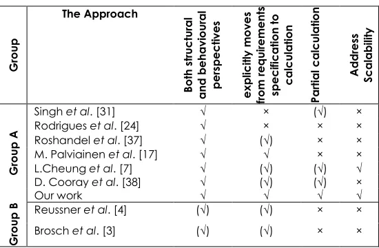
Table 2 summarizes our findings regarding current approaches for design-time reliability engineering. A check mark in parenthesis means that an approach partially supports the feature.

7.0 CONCLUSION AND FUTURE WORK

In this paper, we presented a strategy for scalable modeling and calculation of scenarios reliability based on the system requirements specification. The work is applicable to the early design stage of the software life cycle. The major contribution lies on modeling scenarios in a scalable way by using a scenario language that describes system scenarios in a compact and concise manner potentially results in reduced number of scenarios. Another contribution lies in the calculation, where the well-known “divide and conquer” strategy is followed through the scenarios reliability calculation. Each part of the scenario is tackled separately in the calculation to achieve better traceability and avoid computational complexity in the case of having scenarios consisting of a large number of components. A finite state machine is used to truncate each scenario into its basic elements (component instances) and to reveal their internal states. In the reliability calculation, the failure probabilities of the operations within the component and operations’ invocations that exhibited in the scenarios are utilized as base for the scenario reliability. In summary, the proposed approach may enhance the ability of the current reliability approaches to deal with large software systems.

Table 2 Current approaches for design-time reliability G roup The Approach Bo th s tr uctu ra l a nd b eha vi our a l p er sp ec tiv e s ex p licit ly m ov es from requ irem ents sp ec ificat ion to calcu la tion Pa rtia l c a lcul a tion A d d res s Sc a la b ili ty G roup A

Singh et al. [31] √ × (√) × Rodrigues et al. [24] √ × × × Roshandel et al. [37] √ (√) × × M. Palviainen et al. [17] √ √ × × L.Cheung et al. [7] √ (√) (√) √ D. Cooray et al. [38] √ (√) (√) ×

Our work √ √ √ √

G

roup

B Reussner et al. [4] (√) (√) × × Brosch et al. [3] (√) (√) × ×

Acknowledgement

The authors are very grateful to the Ministry of Education (MOE) Malaysia, under vote no. 4F303, and Universiti Teknologi Malaysia, for their financial support of this research. The authors would also like to thank Embedded & Real-Time Software Engineering Laboratory (EReTSEL) members for their thoughtful and constructive feedback.

References

[1] Lyu, M. R. 2007. Software Reliability Engineering: A Roadmap. IEEE.

[2] Musa, J. D., A. Iannino, and K. Okumoto. 1987. Software Reliability: Measurement, Prediction, Application. McGraw-Hill, Inc.

[3] Brosch, F., et al. 2011. Architecture-Based Reliability Prediction with the Palladio Component Model. IEEE Transactions on Software Engineering. 99: 1-1.

[4] Reussner, R. H., H. W. Schmidt, and I. H. Poernomo. 2003. Reliability Prediction for Component-Based Software Architectures. Journal of Systems and Software. 66(3): 241-252.

[5] Immonen, A. and E. Niemelä. 2008. Survey of Reliability and Availability Prediction Methods from the Viewpoint of Software Architecture. Software and Systems Modeling. 7(1): 49-65.

[6] Krka, I., et al. 2009. A Comprehensive Exploration of Challenges in Architecture-based Reliability Estimation. Architecting Dependable Systems VI. 202-227.

[7] Cheung, L., et al. 2012. Architecture-Level Reliability Prediction of Concurrent Systems. ACM.

[8] Gokhale, S. S. and K. S. Trivedi. 2002. Reliability Prediction and Sensitivity Analysis Based on Software Architecture. IEEE. [9] Cortellessa, V., H. Singh, and B. Cukic. 2002. Early Reliability

Assessment of UML Based Software Models. ACM.

[10] Yacoub, S., B. Cukic, and H. H. Ammar. 2004. A Scenario-Based Reliability Analysis Approach for Component-Scenario-Based Software. Reliability, IEEE Transactions on. 53(4): 465-480. [11] Cukic, B. 2005. The Virtues of Assessing Software Reliability

Early. Software, IEEE. 22(3): 50-53.

[12] Goswami, V. and Y. Acharya. 2009. Method for Reliability Estimation of COTS Components based Software Systems. [13] Hsu, C. J. and C. Y. Huang. 2011. An Adaptive Reliability

Analysis Using Path Testing for Complex Component-Based

Software Systems. Reliability, IEEE Transactions on. 60(1): 158-170.

[14] Fan, Z., et al. 2008. A Novel Model for Component-Based Software Reliability Analysis. In High Assurance Systems Engineering Symposium, 2008. HASE 2008. 11th IEEE. [15] Tyagi, K. and A. Sharma. 2012. A Rule-Based Approach for

Estimating the Reliability of Component-based Systems. Advances in Engineering Software. 54: 24-29.

[16] Kim, Y., et al. 2013. Validating Software Reliability Early through Statistical Model Checking.Software, IEEE. PP(99): 1-1.

[17] Palviainen, M., A. Evesti, and E. Ovaska. 2011. The Reliability Estimation, Prediction and Measuring of Component-based Software.Journal of Systems and Software. 84(6): 1054-1070. [18] Mauw, S., M. Reniers, and T. Willemse. 2001. Message Sequence Charts in the Software Engineering Process. Handbook of Software Engineering and Knowledge Engineering. 1: 437-464.

[19] Pilone, D. 2005. UML 2.0 in a Nutshell. O'Reilly Media, Inc. [20] Diirr, E. and J. van Katwijk. 1992. VDM++, A Formal

Specification Language For Object-Oriented Designs. In Proceedings 6th Annual European Computer Conference, Compeuro.

[21] Harel, D. and R. Marelly. 2003. Come, Let’s Play: Scenario-Based Programming Using Lscs and the Play-Engine. Vol. 1. Springer.

[22] Sibay, G., S. Uchitel, and V. Braberman. 2008. Existential Live Sequence Charts Revisited. In Software Engineering, 2008. ICSE'08. ACM/IEEE 30th International Conference on. IEEE. [23] Harel, D. 1987. Statecharts: A Visual Formalism for Complex

Systems.Science of Computer Programming. 8(3): 231-274. [24] Rodrigues, G., D. Rosenblum, and S. Uchitel. 2005. Using

Scenarios to Predict the Reliability of Concurrent Component-Based Software Systems. Fundamental Approaches to Software Engineering. 111-126.

[25] Sibay, G. E., et al. 2013. Synthesizing Modal Transition Systems from Triggered Scenarios. Software Engineering, IEEE Transactions on. 39(7): 975-1001.

[26] Harel, D. and E. Gery. 1996. Executable Object Modeling with Statecharts. In Proceedings of the 18th International Conference on Software Engineering. IEEE Computer Society.

[27] Ali, A., D. N. Jawawi, and M. A. Isa. 2014. Modeling and Calculation of Scenarios Reliability in Component-Based Software Systems. In Software Engineering Conference (MySEC), 2014 8th Malaysian. IEEE.

[29] Krka, I., et al. 2009. Synthesizing Partial Component-Level Behavior Models from System Specifications. In Proceedings of the 7th Joint Meeting of the European Software Engineering Conference and the ACM SIGSOFT Symposium on the Foundations of Software Engineering. ACM.

[30] Whittle, J. and J. Schumann. Generating statechart designs from scenarios. in Software Engineering, 2000. Proceedings of the 2000 International Conference on. 2000. IEEE. [31] Singh, H., et al. A bayesian approach to reliability prediction

and assessment of component based systems. 2001. IEEE. [32] Roshandel, R., et al. Understanding tradeoffs among

different architectural modeling approaches. in Software Architecture, 2004. WICSA 2004. Proceedings. Fourth Working IEEE/IFIP Conference on. 2004. IEEE.

[33] Goseva-Popstojanova, K., et al. 2003. Architectural-level Risk Analysis Using UML.Software Engineering, IEEE Transactions on. 29(10): 946-960.

[34] Sadi, M. S. et al. 2010. Component Criticality Analysis to Minimizing Soft Errors Risk. International Journal of Computer Systems Science and Engineering. CRL Publishing. 25(5). [35] Wang, W. L., D. Pan, and M. H. Chen. 2006.

Architecture-Based Software Reliability Modeling. Journal of Systems and Software. 79(1): 132-146.

[36] Gokhale, S. S. and K. S. Trivedi. 2002. Reliability Prediction and Sensitivity Analysis Based on Software Architecture. In Software Reliability Engineering, 2002. ISSRE 2003. Proceedings. 13th International Symposium on. IEEE. [37] Roshandel, R., N. Medvidovic, and L. Golubchik. 2007. A

Bayesian Model for Predicting Reliability of Software Systems at the Architectural Level. Software Architectures, Components, and Applications. 108-126.