Computing Robin problem on unbounded simply connected domain via an integral equation with the generalized Neumann kernel

(1)

Computing Robin Problem on Unbounded Simply

Connected Domain via an Integral Equation with the

Generalized Neumann Kernel

Shwan H. H. Al-Shatri

Science Department Institute of Training and Educational

Development in Sualiamni-Iraq

[email protected]

Munira Ismail. Department of Mathematical Sciences

Faculty of Science

Universiti Teknologi Malaysia, Malaysia

[email protected]

Karzan Wakil

Sualimani Polytechnic University-Iraq University of Human Development-Iraq

[email protected]

Abstract: A Robin problem is a mixed problem with a linear combination of Dirichlet and Neumann D-N conditions. The aim of this paper are presents a new boundary integral equation BIE method for the solution of unbounded Robin boundary value problem BVP in the simply connected domain. The method show how to reformulate the Robin boundary value problem BVP as Riemann-Hilbert problem RHP which lead to the system of integral equation, and the related differential equations are also created that give rise to unique solutions. Numerical results on several tests regions by the Nyström method NM with the trapezoidalrule TR are presented to clarify the solution technique for the Robin problem when the boundaries are sufficiently smooth.

Keywords: Robin problem, Riemann-Hilbert problem, Integral equation, Generalized Neumann kernel, Simply connected region.

1. INTRODUCTION

Many applications of the Laplacian differential operator are related to physical geodesy, measurement [1-2], while the application of mixed boundary value problem has been developed only during recent century [3]. In this study the mixed boundary value problem in the literature is the mixed D-N boundary value problem BVP

.

In this paper the applications of the mixed D-N of BVP in potential theory can be seen in [4]. A mixed BVP has mixed D-N type boundary conditions [5-6].

A Robin problem is a mixed BVP with a linear combination of D-N conditions, commonly called a Robin condition [6]. Many analytical methods for computing the Robin BVP for the Laplace’s equation ∆u=0 in a simply connected region are limited to special domains. For general shape region, we have to resort to numerical methods [7–9]. Robin’s condition is also called the third boundary condition in some books such as [10–12].

Robin problem was named after French mathematician called Victor Gustave Robin (1855-1897). He was a professor of applied mathematics, specifically in the field of mathematical physics at Sorbonne University in Paris [13].

At recent days, the interplay of RHP and integral equation with the generalized Neumann kernel GNK has been investigated in [14] for simply connected regions with smooth boundaries and in [15-16] for bounded and unbounded doubly connected and multiply connected regions.

In this paper we are compute the Robin BVP by reducing it to form of RHP, hence as long as the related system of boundary integral equation BIE method. By the additional conditions to the Robin BVP are given to obtain the unique solution.

2. NOTATIONS

AND

AUXILIARY

MATERIAL

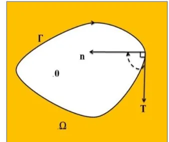
Consider the unbounded Robin problem on an arbitrary simply connected domain Ω with the boundary Γ. It consists of finding a function u harmonic in the domain, continuous on domain and the boundary and satisfies the Robin’s equation. An unbounded simply connected region with clockwise orientation boundary Γ which is a smooth Jordan curve (see Figure 1).

Figure 1 An unbounded simply connected domain Ω. The curve is parameterized by2 -periodic twice continuously differentiable complex function



(

t

)

with non-vanishing first derivative.

(2)

( ( ))

( ) ( ( ))t u t ( ) t u t = ( ) ( ), ( )l t t t 0, ( )t ,

        

n

(1)

where n is exterior normal vector to . If _>₀

) ( ) ( t t





_,

then the Robin BVP has a uniquely solution (see e.g [11, p. 163] and [12, p. 141]).The RHP can be computed a BIE with the GNK. This paper, relate the Robin problem with the RHP. We are define the real kernels in GNK and as imaginary kernel in GNK and real parts in GNK [8-9].

The RHP is consists of finding a function

g

is analytic

in the domain Ω.

.

=

]

[

Re

Ag



Theorem 1. ([8-13]) If

g

in the RHP equation

Re[Ag]= is a solution of the RHP with BVP

,

i

=







Ag

(2)

Then from equation (2) the imaginary part



is satisfies the BIE





N



= -M



. (3)

In this work the solubility of BIE with the GNK is specific by the index of the peroidic function

A

(

t

)

[9].

Theorem 2. ([14] Cauchy Integral Formula CIF) Let

f

be a function that is analytic everywhere in



and on a simple closed contour



. If z is any point in side the domain . Then the CIF is

∫ {



(4)

3. METHODOLOGY

OF

ROBIN

PROBLEM

We consider the methodology of computingthe Robin BVP with the Robin condition in an unbounded simplyconnected region as shown in Figure 2.

Figure2 Flowchart of Methodology

It can be shown that the Robinproblem (1) cab be reformulated as [15-16]:

0 0

1 2

0 0

1 2 1 2 1 2

( ) | ( ) | cos ( ) ( ) | ( ) | sin ( )

( ) ( ( )) = i

( ) ( )

( ) cos ( ) ( ) sin ( )

i i

( ) ( )

= ( ) i ( ) i ( ) ( ) i

= ( ( ) ( ) ) i( ( ) ( ) ),

t t

l l

A t g t d d

d d c c

t t t t c c

t t c t t c

                     _     _                               

tJ,

(5)

Where

c

₁,

c

₂, are unknown real constants in H, and

, , ) ( ) ( cos | ) ( | ) ( := ) ( 0

1 d t J

l

t



t  

         (6) , , ) ( ) ( sin | ) ( | ) ( := ) ( 0

2 d t J

l

t



t  

         (7)

Are known functions in H, and

, , ) ( ) ( cos ) ( := ) ( 0

1 t d t J

t 















(8) , , ) ( ) ( sin ) ( := ) ( 0

2 t d t J

t 



        (9)

Are unknown functions in H [15-16].Then the equation (5) can be written briefly describe as equation (5) where

1 2

1

(

)

(

)

=

)

(

t



t





t



c



(10)

2 1

2

(

)

(

)

=

)

(

t



t





t



c



(11)

From the equation (5) the real part produce the RHP.

The periodic function

A

(

t

)

=

e

i(t)is not periodic in general.To stratify the result of Theorem 1, the periodic function

A

(

t

)

must be satisfy the condition









(2

)



(0)

=

2

. Then by the Theorem 1 implies that equation(2) becomes the integral equation

. ) ) ( ) ( ( = ) ) ( ) ( )(

(IN 2 s 1 s c2 M1 s 2 s c1 (12)

. ) ( ) ( ) ( = ) ( ) ( ) ( )

(IN 1 s M2 s Mc1 INc2 M1 s  IN2 s (36)

Then applying both integral operatorsN andM[8,9], we obtain ), ) ( )) ( ), ( ( ) ( ( ) ( )) ( ), ( ( )) ( ), ( ( ( )) ( ), ( ( ) ( )) ( ), ( ( ) ( )) ( ), ( ( ) ( 2 2 1 2 2 1 2 1 1



         J J J J J J dt t t s N s dt t t s M dt c t s N c dt c t s M dt t t s M dt t t s N s                   (13)

The system of integral equations (13) is in two unknown real functions



₁

(

t

),



₂

(

t

)

also two unknown real constants

c

₁

,

c

₂. In this work by both functions



₁

(

t

)

(

2

t



are given in equations (7),(8) respectivly,have a condition in the form of a differential equation

, 0, = ) ( )) ( ( cos ) ( )) ( (

sin



t



₁' t 



t



₂' t tJ (14)

(3)

1(0) = 0,

 and



₂

(0) = 0.

(15)

For the exterior Robin problem, we have which implise

g

(



)

. Then applying the CIF for unbounded domain



in the Theorem 2, we have together with (5), (10) and (11), yields

. , )

( ) (

) ( )] ) ( ) ( ( i ) ( ) ( [ i 2

1 =

) ( ) (

)) ( ( i 2

1 = ) ( i 2

1 = ) (

2

0

2 1 2 1 2

1 _dt _t _J

t t A

t c t t c t t

dt t t

t g d

g g

 

    



  



   

 

 

   

 



 ₍₁₆₎

Thus

g

(



)

, implies that

∫

Re ̇ +i Im ̇ (17) The real part and imagenary part of equation (17) gives more conditions as

∫ ̇ ∫ ̇ +c1∫

̇

+ (18)

c2∫ ̇

= ∫ ̇

∫ ̇

and

∫ ̇

∫ ̇ +c1∫ ̇

- (19)

c2∫ ̇

=∫ ̇

-∫ ̇

Finally to compute the Robin BVP (1) on exterior domain, we compute for c1 and c2 from (14),(14), (15), (18) and (19). Then we compute from (5).Furthermore, by the relationship of g= -if we get ( ) ( ) and hence ( ) ( ) . The interior values of ( )can be calculate with the CIF (4) which yields when the values z in the exterior domain .

4. IMPLEMENTATION

The functions in the form of both

A

(

t

)

and



(

t

)

are





2

periodicfunction respectively, then the integral equation in (12) can be better discretized in this study on an equidistant connection by the Nystrom method NM with the Trapezoidal rule TR by using

n

equidistant nodes [17]. Since

M

=

M

₁



K

, in this work the singular kernel K are discretized using the Wittich’s

method WM [18]. Hence, now we have

n

equations in

2

2 n



unknowns variables

2 1 2 2 2 1 2 1 2 1 1

1(t),(t ),...,(tn), (t), (t ),..., (tn),c,c

 _.(20)

This equation (14) will be discretized to obtain n more equations [19]. We now have

2 n

equations in

2 n



2

in unknowns variables (20). For the Robin BVP on unbounded simply connected domain, we also have two conditionsfrom (15), we obtained

(2

n



2)

by

.

2)

(2

n



Finally, the two more equations from (18) and (19) are respectively add to give a (2n+4) by (2n+2) linear system.

In this case, the obtained linear systems are computed by using the MATLAB softwere (2011a), 32-bit operating system.

From the computed solutions

1 2 1 2

1(t),



(t),



(t),



(t),c



and

c

₂, the approximate

boundary values of the analytic function f_n(



(t)) are

calculated using the formula

. ) ) ( ) ( ( i ) ) ( ) ( ( = )) (

( 2 1 2_i ₍₎ 1 2 1

t n

e

c t t c

t t t

f      _   

(21)

We approximate interior values of the equation (21) are calculated with the CIF in the form of

.

i 2

1 1

) ( i 2

1 ) ( = ) (

z d

d z f f

z f

J J

 





  

 

 

(22)

Here f(∞) = 0 ,then approximate the integral in (22) for exterior region [20] then computed by using the trapezoidal rule.

5. NUMERICAL

RESULT AND

EXAMPLE

Considered two examples computing of Robin BVP in exterior domain.

Example1. In this examplewe coonsider the domain are bounded by

.

2

0 ,

)

(

:













t

e

t

it

For



(t),



(t), u(t) in (1), we choose

,

sin

2 .

0

1 )

(

t





t



and



(

t

)



1 .

Thefunction

l

(

t

)



2 cos

t



0 .

5 cos

2

t

in (1) the exact

solution in this example is

(4)

The real constantes are c1=0 andc2= -1. For this example, ()_ (0.5sin), _ _[0,2].

J t e

t

A it t

Table 1 and Table 2 are lists the maximum error norm

|| ( ( ))

u



t



u

_n

( ( )) ||



t

_ and the error || ( )f z f zn( ) ||

respectively are plotted in Figure 3 and Figure 4 as shown below with n=512.

Table 1: The error || ( ( ))ut u_n( ( )) ||t _ for Example 1.

Table 2: Absolute error _| _f₍_z₎ _f ₍_z₎_|

n

 at some selected points on domain .

n -1.3+1.1i -1.2+1.2i -1-1.5i 32 5.49(-5) 7.36(-5) 7.85(-5) 64 6.15(-6) 7.29(-6) 8.34(-6)

128 256 512

4.75(-7) 3.16(-8) 2.02(-9)

5.53(-7) 3.66(-8) 2.33(-9)

6.16(-7) 4.06(-8)

2.59(-9)

Figure 3 The error |u(z) − (z)| for Example 1 with n= 512.

Figure 4 The approximation solution for Example 1 with n= 512.

Example2. In this example also we coonsider the domain are bounded by

.

2

0 )

cos

5 .

0

8 .

1 (

)

(

:















t

e

t

it

In (1) the exact solution of this example is

z z

f( ) 1,

The real constants are c1=0, c2=-0.4348.

Table 3 and Table 4 are lists the maximum error norm

|| ( ( ))

u



t



u

_n

( ( )) ||



t

 and the error || ( )f z f zn( ) || respectively are plotted in Figure 5 and Figure 6 as shown below with n=512.

Table 3: The error || ( ( ))ut u_n( ( )) ||t _for Example 2.

n

32 9.45 (-3)

64 4.29 (-4)

128 256 512

1.84 (-5) 1.32 (-7) 1.01 (-8)

Table 4: Absolute error | f(z)f_n(z)| at some selected points on domain .

n 1.1+1.1i -1.1-1.1i 1.1-1.1i -1.1+1.1i

32 2.70(-3) 2.10(-3) 1.40(-3) 1.80(-3) 64 1.12(-4) 9.63(-5) 1.07(-4) 9.41(-5) 128

256 512 1024

7.06(-6) 4.40(-7) 4.77(-8) 1.72(-9)

6.00(-6) 3.75(-7) 2.34(-8) 1.40(-9)

6.94(-6) 4.34(-7) 2.71(-8) 1.69(-9)

5.92(-6) 3.69(-7) 2.30(-8) 1.43(-9)

Figure 5 The error |u(z) − (z)| for Example 2 with n= 512.

Figure 6 The approximation solution for Example 2 with n= 512.

6. CONCLUSIONS

We have solved exterior Robin problems in simply connected domain with smooth boundaries using a

n

32 9.20 (-3)

64 3.87 (-4)

128 256 512 1024

(5)

combination of a system of integral equation and the differential equations. In this paper, the integral equation is discretized by the Nystrom method NM with the Trapezoidal rule TR and the Wittich’s method WM in [15-16], however in this study the differential equation is discretized in [19]. In conclusion, the presented numerical results clarify that our method can be used to make approximations [20] of good accuracy and best results.

7. REFERENCES

[1] W. Heiskanen,H. Moritz. Physical Geodesy. San Francisco / London. 1967

[2] W. Fang, Z. Suxing. Numerical recovery of Robin boundary from boundary measurements for the Laplace equation.Journal of Computational and Applied Mathematics, 224:573-580, 2009.

[3] K. Gustafson, A. Takehisa. The third boundary condition was it Robin’s?The Mathematical Intelligencer, 20:63-71, 1998.

[4] I. N. Sneddon.Mixed Boundary Value Problems In Potential Theory. North-Holland. 1966

[5] M. M. S. Nasser, A. H. M. Murid, M. Ismail, E. M. A. Alejaily. Boundary integral equations with the generalized Neumann kernel for Laplace’s equation in multiply connected regions. Appl. Math. Comput, 217:4710-4727, 2011.

[6] S. A. A. Alhatemi, A. H. M. Murid, M. M. S. Nasser. A boundary integral equation with the generalized Neumann kernel for a mixed boundary value problem in unbounded multiply connected regions.Boundary Value Problems, 1: 1-17, 2013. [7] M. M. S. Nasser. Numerical conformal mapping via

a boundary integral equation with the generalized Neumann kernel. SIAM Journal on Scientific Computing, 31:1695-1715, 2009.

[8] R. Wegmann, A. H. M. Murid, M. M. S. Nasser. The Riemann-Hilbert problem and the generalized Neumann kernel.Journal of Computational and Applied Mathematics, 182:388-415, 2005.

[9] R. Wegmann, M. M. S. Nasser.The Riemann-Hilbert problem and the generalized Neumann kernel on multiply connected regions.Journal of Computational and Applied Mathematics, 214:36-57, 2008.

[10]T. Petrila. Complex value boundary element method for some mixed boundary value problems. Studia Univ, Babes-Bolyai, Informatica, 44:37-42, 1999. [11]R. M. M. Mattheij, S. W Rienstra, J. H. M. ten Thije

Boonkkamp. Partial Differential Equations Modeling, Analysis, Computation.SIAM. 2005 [12]S. Salsa.Partial Differential Equations in Action

From Modeling to Theory.Springer Science and Business Media. 2008

[13]M. M. S. Nasser. The Riemann-Hilbert problem and the generalized Neumann kernel on unbounded multiply connected regions. The University Researcher Journal, 20: 47-60, 2009.

[14]F. D. Gakhov. Boundary Value Problem. Oxford Pergamon Press. 1966

[15]S. H. H. Al-Shatri, A. H. M. Murid, M. Ismail, M. I. Muminov. Solving Robin problems in multiply connected regions via an integral equation with the generalized Neumann kernel.Boundary Value Problem.2016, 1-23,2016.

[16]S. H. H. Al-Shatri, A. H. M. Murid, M. Ismail. Solving Robin problems in bounded doubly connected regions via an integral equation with the generalized Neumann kernel. AIP Conference Proceedings.1750,1, p. 030004) 2016.

[17]K. E. Atkinson. The Numerical Solution of Integral Equations of the Second Kind. Cambridge: Cambridge University Press. 1997

[18]D. Gaier. Konstruktive Methoden der Konformen Abbildung.Berlin-Göttingen-Heidelberg. 1964 [19]M. Abramowitz, I. E. Stegun. Handbook of

Mathematical Functions, with Formulas, Graphs, and Mathematical Tables. Courier Corporation. 1964