APPLICATION OF MASTER CURVE METHODOLOGY IN THE
DUCTILE TO BRITTLE TRANSITION REGION FOR THE MATERIAL
20MnMoNi55 STEEL
S. Bhowmik1, A. Chatterjee1, S.K. Acharyya1, P. Sahoo1, S. Dhar1, J. Chattopadhyay2 1 Department of Mechanical Engineering, Jadavpur University, Kolkata – 700032 2 Reactor Safety Division, Bhaba Atomic Research Centre, Trombay, Mumbai - 400085
E-mail of corresponding author: [email protected], [email protected]
ABSTRACT
Fracture toughness is an important material property to assess the critical load for structural integrity of reactor pressure vessel steel. In this paper, Master Curve method proposed by Kim Wallin is used to estimate the fracture toughness of 20MnMoNi55 steel in the ductile to brittle transition regime. Reference temperature (T0) is
evaluated using both single temperature and multi-temperature method for one inch thick compact tension (1T-CT) and 1/2-CT specimens. Reference temperature (T0) is also determined from Charpy V-notch test data and compared.
Effect of selection of temperature range and number of test temperatures on the value of T0 is also studied. The
correction proposed for thickness adjustment has been verified. It is observed that Charpy test results yield lower values of unirradiated T0 compared to 1T-CT specimen tests. It is also observed that most of the fracture toughness
values fall between 5% and 95% boundary of fracture toughness curves for all the evaluations.
INTRODUCTION
Both the scatter of fracture toughness in the transition zone and temperature dependence of fracture toughness is captured and expressed through Master curve method [3]. The master curve methodology is based on modelling cleavage fracture toughness at a fixed temperature in the transition with a 3-parameter Weibull distribution and the proposition that the shape of the fracture toughness vs. temperature curve is identical for all ferritic steels but having difference in absolute position in the temperature axis. The particular position of the curve for a particular steel is given in terms of the fracture toughness reference temperature (T0) which is defined as the
temperature at which the median fracture toughness for a 1T (one inch thick) compact tension (CT) specimen equals to 100 MPa√m [4]. Thus the master curve defines both the variation of the median value of fracture toughness with temperature and the scatter of fracture toughness about this median value. The master curve together with a reference temperature (T0) value define the complete transition fracture toughness curve in a manner appropriate for
use in both probabilistic and deterministic analysis. The master curve method is also used to construct a bounding curve on the fracture toughness. Typically a bounding curve with a 95% degree of confidence is used as lower bound on the fracture toughness. In this paper Master Curve method proposed by Kim Wallin is used to estimate the fracture toughness of the 20MnMoNi55 material in the ductile to brittle transition regime. Transition zone for the material is identified by Charpy impact test results. Then tensile properties are measured at different temperatures in the transition zone. Fracture toughness of 1T-CT and 1/2-CT specimens of the 20MnMoNi55 material is measured at different temperatures covering upper shelf to transition. For Cleavage fracture in the transition zone Weibull Parameters (Kmin, K0 ) are estimated from fracture toughness results obtained from the experiments. Then both the
single temperature and multi-temperature analysis are used to determine the reference temperature for master curve of the material. The correction proposed for thickness adjustment has been verified. All the propositions described in Master curve methodology are verified for this particular steel and found to be satisfactory. Proposition regarding Kmin is validated. Single and multi-temperature reference temperature estimation algorithm yield equivalent
estimates. It is found master curves obtained from single temperature analysis fall between 5% and 95% bound fracture toughness curves obtained from multi-temperature evaluation. The effects of specimen thickness, a/w, testing temperature range and no. f test temperatures used to compute T0 on the value of T0 are also studied.
MASTER CURVE ANALYSIS
Master Curve Analysis for Charpy Test Data
Wallin showed that the brittle fracture probability Pf for a given temperature in the transition region is
⎥ ⎥ ⎦ ⎤ ⎢ ⎢ ⎣ ⎡ ⎟⎟ ⎠ ⎞ ⎜⎜ ⎝ ⎛ − − − − = 4 min 0 min JC
f K K
K K exp 1
P (1)
where KJC value is converted value of JC equal to critical K obtained from JC in MPa√m, K0 is a scale parameter
dependent on the test temperature and specimen thickness, and Kmin is the minimum possible fracture toughness. In
this study, Barsom and Rolfe’s [5] correlation has been used to estimate the fracture toughness transition curve based on experimental Charpy absorbed energy as given below.
(
)
324 2
IC 2.2 10 CVN E
K = × − (2)
The fracture toughness values obtained from Eq. (2) have been normalized to those of the 1T size using the following equation.
[
]
41 0 1T min IC(X) min
JC(1T) K K K BB
K ⎟⎟ ⎠ ⎞ ⎜⎜ ⎝ ⎛ − +
= (3)
where B0 is thickness of the tested specimen (side grooves not considered) in mm, B1T is the thickness of 1T-CT
specimen [4, 6].
Master Curve Analysis for Fracture Test Data
The transition curve definition for ferritic steels, as specified in ASTM E1921 was originally derived in 1991 from data measured on various quenched and tempered structural steel. The temperature dependence of the median fracture toughness in the transition region can be estimated from [7],
(median)
[
(
0)
]
JC 30 70exp0.019T T
K = + − (4)
Once T0 is known for a given material, the fracture toughness distribution can be obtained as a function of
temperature through Eqs. (1) and (4). Now both upper and lower tolerance bounds can be calculated using following equation [8].
( )
{
[
(
0)
]
}
4 1
.XX 0
JC 20 ln 1 01 11 77exp0.019T T
K .XX + −
⎥ ⎥ ⎦ ⎤ ⎢ ⎢ ⎣ ⎡ ⎟⎟ ⎠ ⎞ ⎜⎜ ⎝ ⎛ − +
= (5)
where 0.XX represents the cumulative probability level.
Finally T0 is compared by rearranging Eq. (4). The KJC limit is calculated according to the ASTM E1921 standard.
Evaluation of T0 from Single Temperature Test Data
For single temperature evaluation, the estimation of the scale parameter K0, is performed according to
following equation [9, 10].
(
)
min 4 1 N 1 i 4 min JC(i)0 N K
K K K + ⎥ ⎥ ⎦ ⎤ ⎢ ⎢ ⎣ ⎡ − =
∑
= (6)
Here KJC(i) is the individual KJC(1T) value and N is the number of KJC values. The fracture toughness for a median
(50%) cumulative probability of fracture is determined using the following equation.
(
)( )
41 min 0 min
JC(median) K K K ln2
K = + − (7)
Now the KJC(median) value determined for the data set at test temperature is used to calculate T0 at KJC(median) of 100
⎟⎟ ⎠ ⎞ ⎜⎜ ⎝ ⎛ − ⎟ ⎠ ⎞ ⎜ ⎝ ⎛ − = 70 30 K ln 0.019 1 T
T0 JC(median) (8)
Evaluation of T0 from multi-temperature test data
For multi-temperature evaluation the determination of T0 is performed with KJC values distributed over a
restricted temperature range, namely, T0 = ±500C. The value of T0 is evaluated by an iterative solution of the
following equation [3].
(
)
[
]
(
)
[
]
(
{
)
[
[
(
(
)
]
}
)
]
∑
=∑
= + − = − − − − + − N 1 i N 1 i 5 0 i 0 i 4 min JC(i) 0 i 0 i i 0 T T 0.019 77exp 11 T T 0.019 exp K K T T 0.019 77exp 11 T T 0.019 exp δ (9)Here Ti is the test temperature corresponding to KJC(i) and δi is the censoring parameter.
δi = 1, if the KJC(i) datum is valid. and δi = 0, if the KJC(i) datum is not valid and censored.
MATERIAL DETAILS
The material used in the present work is 20MnMoNi55 RPV applications steel. It is a German designated material received from Bhaba Atomic Research Centre, Mumbai. The different chemical compositions of the material are given in Table 1.
Table 1: Chemical composition of 20MnMoNi55 steel.
Name of element C Si Mn P S Al Ni Mo Cr Nb
% composition (in weight) 0.20 0.24 1.38 0.011 0.005 0.068 0.52 0.30 0.06 0.032
EXPERIMENTAL DETAILS
For determining master curve various experiments has been performed on the 20MnMoNi55 RPV steel. Tensile tests are performed on round bar specimen according to ASTM E8 standard at different temperatures in the range between 220C and -1400C to evaluate the yield strength, ultimate strength and modulus of elasticity of the
material at different temperatures. All the tensile tests are done in the cryo-chamber attached to a computer controlled Universal Testing Machine with 100 kN grip capacity. The required zero and sub-zero test temperature are attained by flowing liquid nitrogen from fully automated self pressurized Dewar flask of 120 L capacity. To determine Charpy absorbed energy of the material Charpy impact test has been done according to ASTM E23 method with eleven numbers of specimens at temperature 250C, 80C, –100C, –270C, –450C, –620C, –800C, –970C, –
1150C, –1320C and –1500C.
The fracture toughness tests in this investigation are performed on standard 1T-CT and 1/2-CT specimen. All the CT specimen are machined according to ASTM E399-90 standard and pre-crack is introduced at room temperature according to ASTM E647 standard in the range of a/W = 0.45 – 0.50. All the pre-cracking experiments are carried out on servo-hydraulic universal testing machine using commercial da/dN (Fatigue crack growth rate per cycle) software at stress ratio (R) of 0.02 using initial frequency of 10 Hz and with a constant ΔK (increment stress intensity factor) of 30 MPa√m and later on the frequency is increased to 15 Hz. Now to determine J-integral values, the pre-cracked specimens are tested at different temperature range between 220C and –1400C. The J
C fracture
toughness program is used for J-integral testing to obtain J–Δa data on universal testing machine according to ASTM E1820. The required zero and sub-zero test temperature are attained by flowing liquid nitrogen.
RESULTS AND DISCUSSION
Tensile Test Results
The relations between yield and ultimate strength with test temperature are derived using best fit curve and the equations are given below.
Yield strength, σys =0.0112T 2 −0.0431T +494.01 (10)
Ultimate strength, σus =0.0058T 2 −0.6817T +644.81 (11)
Charpy Test Results and Master Curve from Charpy Test Data
From the test results, it is found that the Charpy absorbed energy values start decreasing with decrease in temperature at about 00C and the sharp slope continues up to –1000C and then gets saturated on further decrease in
temperature. The test results fit well with the tangent hyperbolic curve (Fig.1),
⎟ ⎠ ⎞ ⎜
⎝
⎛ +
+ =
43.3 47.3 T 134.5 142
CV (12)
where CV stands for Charpy impact energy in Joule and T is the test temperature in 0C. Initial estimation of master
curve reference temperature (T0 = T41J – 240C ) for 1T specimen is found to be –1140C . From the Charpy transition
curve of the material, the linear elastic fracture toughness is estimated and finally the 1T-CT equivalent elastic plastic fracture toughness transition curve of the material is obtained. The KJC values at different temperature from
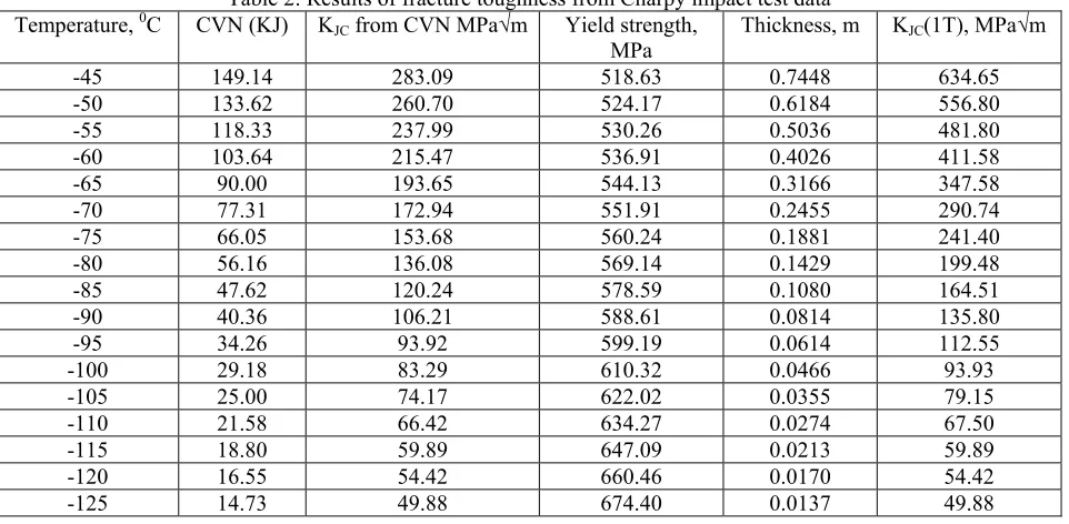
Charpy impact test are listed in Table 2.
Table 2: Results of fracture toughness from Charpy impact test data Temperature, 0C CVN (KJ) K
JC from CVN MPa√m Yield strength,
MPa Thickness, m KJC(1T), MPa√m
-45 149.14 283.09 518.63 0.7448 634.65
-50 133.62 260.70 524.17 0.6184 556.80
-55 118.33 237.99 530.26 0.5036 481.80
-60 103.64 215.47 536.91 0.4026 411.58
-65 90.00 193.65 544.13 0.3166 347.58
-70 77.31 172.94 551.91 0.2455 290.74
-75 66.05 153.68 560.24 0.1881 241.40
-80 56.16 136.08 569.14 0.1429 199.48
-85 47.62 120.24 578.59 0.1080 164.51
-90 40.36 106.21 588.61 0.0814 135.80
-95 34.26 93.92 599.19 0.0614 112.55
-100 29.18 83.29 610.32 0.0466 93.93
-105 25.00 74.17 622.02 0.0355 79.15
-110 21.58 66.42 634.27 0.0274 67.50
-115 18.80 59.89 647.09 0.0213 59.89
-120 16.55 54.42 660.46 0.0170 54.42
-125 14.73 49.88 674.40 0.0137 49.88
Six fracture toughness dataset have been taken from the Charpy impact test data. The dataset are selected in the range from 100 MPa√m to 300 MPa√m (Kim et al, 2002) and these data are used to determine the reference temperature T0 to generate master curve. The reference temperature value T0 = –1220C and the fracture toughness
curve are shown in Fig. 2.
J-integral Test Results
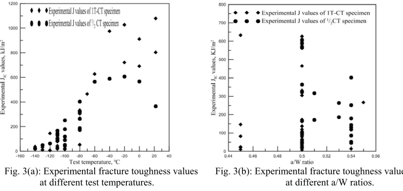
J-integral test is performed according to ASTM E399-90 standard on 1T and 1/2-CT specimens at different temperatures in the range between 220C to –1400C and a/W ratio. All the experimental result using 1T-CT and
1/2-CT specimen at different temperature and different crack length are shown in Fig. 3(a) and 3(b).
Fig. 3(a): Experimental fracture toughness values Fig. 3(b): Experimental fracture toughness values
at different test temperatures. at different a/W ratios.
The fracture toughness values for only those specimens which have undergone brittle failure have been considered for master curve.
Table 3. Values of Reference temperature T0 in 0C
Single temperature Specimen
-80 0 C -110 0 C Multi temperature
Full CT -130 -129
Half CT -126 -130 -126
Combined full
and half CT -130
T0 Estimation at Temperature –800C
The master curve combining both the specimens at –800C is shown in Fig. 4(a) and 4(b).
Fig. 4(a): Master curves at –800C test temperature Fig. 4(b): Master curves at –800C test temperature
for 1/2-CT specimen. for 1T and 1/2-CT combination.
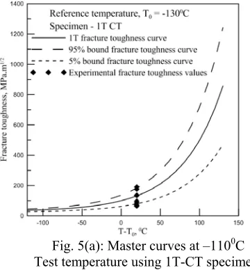
T0 Estimation at Temperature –1100C
Fig. 5(a): Master curves at –1100C Fig. 5(b): Master curves at –1100C
Test temperature using 1T-CT specimen test temperature using 1/2-CT specimen.
T0 Estimation using Multi-temperature Evaluation
In case of multi temperature evaluation different temperature sequences have been considered. The value of T0 is –1290C for 1T-CT specimen. The corresponding master curve is shown in Fig. 6(a). Similarly the value of T0
using multi-temperature method is –1260C for 1/2-CT specimen. The corresponding master curve is shown in Fig.
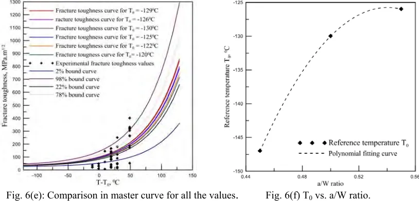
6(b). A number of master curves are obtained for the same material using different methods and specimens. All these curves are presented in the Fig. 6(e) for comparison with the master curve obtained using 1T and 1/2-CT specimens combined and using multi-temperature method.
Fig. 6(e): Comparison in master curve for all the values
.
Fig. 6(f) T0 vs. a/W ratio.Effect of Test Temperature Combination and Temperature Range on Reference Temperature
The value of T0 is estimated using 1T-CT and 1/2-CT specimen by multi-temperature evaluation for
different combination of test temperature. When the data of two test temperature is used for evaluating T0, the value
of T0 varies from –1280C to –1330C for 1T-CT specimen and from –1240C to –1290C for 1/2-CT specimen. When
the data of three test temperatures are used the value of T0 varies between –1270C to –1310C for 1T-CT specimen
and –1240C to –1280C for 1/2-CT specimen. Also the range is –1260C to –1300C for 1T-CT and –1230C to –1260C
for 1/2-CT when data of four test temperature is used. Pearson’s product-moment correlation coefficient is used to measure the dependence of T0 for both the cases of 1T-CT and 1/2-CT specimen with test temperature range. From
the analysis it is has been found that as the temperature range increases the value of T0 from consistent for both the
specimen.
Effect of a/W for Fixed Thickness on Reference Temperature T0
Specimens from both 1T-CT and 1/2-CT having same a/W ratio are taken together in a sample to evaluate T0. KJC values for 1/2-CT are adjusted with size correction. Thus values of T0 are evaluated for a/W of 0.45, 0.50
and 0.55. From the result it is observed that as the value of a/W increases the value of T0 also increases. Hence a
dependence of T0 on a/W ratio is found from the results.
Kmin validation
The single temperature data is plotted into the probability diagram; it must be ordered by rank and designated rank probabilities. The three common estimates of the rank probability are
Prank=[(i-0.5)/n] 14(a) Prank=[i/(n+1)] 14(b) Prank = [(i-0.3)/(i+0.4)] 14(c)
In Fig. 7(a) linear fitting is used to fit the experimental fracture toughness data to verify the Kmin value using
rank probability Eq.14(a). This fitting does not satisfy the Kmin estimation, need more experimental value. In Fig.
7(b) linear fitting is used to fit the experimental fracture toughness data to verify the Kmin value using rank
probability Eq. 14(b). This fitting nearer to the Kmin estimation, satisfy the experimental value. Similarly linear
fitting is used to fit the experimental fracture toughness data to verify the Kmin value using rank probability Eq.
14(c). This fitting does not satisfy the Kmin estimation, need more experimental value.
CONCLUSION
Fracture toughness of 20MnMoNi55 steel is evaluated by Charpy impact test method and master curve method. Both the single temperature and multi-temperature analysis are used to determine the reference temperature for master curve of the material on CT specimen. From the present study, the following conclusions can be made:
i) Like other ferritic RPV steels, this material also shows the scatterness of the fracture toughness values in DBT region.
ii) Brittle fracture is observed at and below –800C.
iii) As expected, the reference temperature T0 obtained from CT specimen fracture tests is less than the Charpy
impact test data. The variation in T0 between these two methods is ±50C.
iv) Although multi-temperature method is more effective way in estimating reference temperature, in the present study both single and multi-temperature estimation yield close result.
v) In case of multi-temperature evaluation T0 is found to be more consistent when number and range of test
temperatures increase.
vi) Considering fracture toughness curve derived from multi-temperature method as reference curve, it is found that most of the fracture toughness values fall within 95% and 5% bound confidence levels of the reference curve.
vii) For negligible variation in reference temperature derived from different methods and differently sized specimen one can derive the reference temperature by single temperature evaluation method and 1/2-CT specimens to reduce time, material utilization and cost also.
REFERENCES
[1] Wallin, K., The size effect in KIC result. Engineering Fracture Mechanics, Vol. 22, 1985, pp. 149-163.
[2] Wallin, K., The scatter in KIC result. Engineering Fracture Mechanics, Vol. 19, 1984, pp. 1085-1093.
[3] Viehrig, H.-W., Boehmert, J., Dzugan, J., Some issues by using the master curve concept. Nuclear
Engineering and Design, Vol. 212, 2002, pp. 115 – 124.
[4] Kim, S.H., Park, Y.W., Kang, S.S., Chung, H.D., Estimation of fracture toughness transition curves of RPV
steels from Charpy impact test data. Nuclear Engineering and Design, Vol. 212, 2002, pp. 49-57.
[5] Barsom, J.M., Rolfe, S.T., Correlations between KIC and Charpy V-notch test results in the
transition-temperature range. ASTM STP, Vol. 466, 1970, pp. 281-302.
[6] Kim, S., Lee, S., Lee, B. S., Effects of grain size on fracture toughness in transition temperature region of
Mn-Mo-Ni low-alloy steels. Materials and Engineering, Vol. A359, 2003, pp. 198 – 209.
[7] Serrano, M., Perosanz, F.J., Lepe a, J., Direct measurement of reactor pressure vessel steels fracture
toughness: Master Curve Concept and instrumented Charpy. V-test. International Journal of Pressure Vessels and Piping, Vol. 77, 2000, pp. 605 – 612.
[8] Brumovský, M., Check of Master Curve application to embrittled RPVs of WWER type reactors. International Journal of Pressure Vessels and Piping, Vol. 79, 2002, pp.715-721.
[9] Rosinski, S.T., Server, W.L., Application of the Master Curve in the ASME Code. International Journal of
Pressure Vessels and Piping, Vol. 77, 2000, pp. 591 – 598.