Comparisons between Computation and Experiment for Shock-Layer Radiation.

(1)

ABSTRACT

MCCORKLE, EVAN REID. Comparisons between Computation and Experiment for Shock-Layer Radiation. (Under the direction of Hassan Hassan.)

In attempts to validate NEQAIR, a tool used by NASA Ames Research Center for the

calculation of radiative heating, a study was undertaken that ventured to understand and explain

the discrepancies between computations and the experimental spectroscopy of the NASA Ames Electric Arc Shock Tube facility. A method is described by which the spatially-spectrally resolved

spectrographic data of shock-layer radiation can be reduced to spectrally-only resolved data

representative of the radiation behind the shockwave. Workflows are created to allow the linking of different computational flowfields to NEQAIR. These include Chemical Equilibrium with

Applications (CEA), producing a simple post-shock equilibrium flowfield with no spatial variation, and the Data-Parallel Line Relaxation computational fluids code (DPLR), producing a complex

thermochemical nonequilibrium flowfield with both axial and radial spatial variations. In an

attempt to resolve discrepancies through radiation modeling changes, updates to the NEQAIR codebase and databases were undertaken. These included the addition of new molecular bands,

changes in atomic Stark broadening, a sync of atomic bound-bound transitions from the NIST

Atomic Spectra database, and an application of atomic bound-free cross-sections from The Opacity Project. Another attempt was made to resolve discrepancies through flowfield modeling changes,

i.e. by using DPLR and allowing for spatial variation and nonequilibrium effects. In this way, the

effect of the boundary-layer on calculated radiation was studied. While the update of NEQAIR did little, the DPLR flowfield method had some effect in closing the gap between computation

(2)

c

(3)

Comparisons between Computation and Experiment for Shock-Layer Radiation

by

Evan Reid McCorkle

A thesis submitted to the Graduate Faculty of North Carolina State University

in partial fulfillment of the requirements for the Degree of

Master of Science

Aerospace Engineering

Raleigh, North Carolina

2010

APPROVED BY:

Stephen Campbell Hong Luo

Hassan Hassan

(4)

BIOGRAPHY

Evan McCorkle was born in 1985 to Gary and Leslie McCorkle in Charlotte, North Carolina. After

his pastoral youth, he moved to the City of Oaks (Raleigh, North Carolina) to study Aerospace

Engineering at North Carolina State University. After finishing his undergraduate degree, he enrolled in the graduate program under the direction of Professor Hassan Hassan. During this

program, several fruitful summers were spent interning at NASA Ames Research Center under

(5)

TABLE OF CONTENTS

List of Figures . . . iv

Chapter 1 Introduction . . . 1

1.1 Motivation . . . 1

1.2 Methodology . . . 2

Chapter 2 Equilibrium Comparisons . . . 6

2.1 Workflow . . . 6

Chapter 3 Updated Computational Models . . . 8

3.1 Updates . . . 8

Chapter 4 Nonequilbrium Comparisons . . . 11

4.1 Workflow . . . 11

Chapter 5 Results & Discussion. . . 16

5.1 Nomenclature . . . 17

5.2 Sample EAST Spectroscopy . . . 17

5.3 Updated NEQAIR . . . 19

5.4 DPLR . . . 20

5.5 Conclusions . . . 23

(6)

LIST OF FIGURES

Figure 1.1 Shocktube setup/nomenclature . . . 4

Figure 1.2 Shock structure after diaphragm bursts . . . 4

Figure 1.3 Spectroscopy setup . . . 5

Figure 1.4 Spectrographs record spectral and axial variation . . . 5

Figure 2.1 Equilibrium (CEA) workflow . . . 7

Figure 4.1 Nonequilibrium (DPLR) workflow . . . 14

Figure 4.2 Variation of Computational (DPLR) Shock-Front Speed . . . 15

Figure 5.1 Shock structure after diaphragm bursts . . . 23

Figure 5.2 Spectroscopy setup . . . 24

Figure 5.3 Example of EAST Spectroscopy with Annotated Spatial-Averaging Region 25 Figure 5.4 Example of EAST Radiance Profile . . . 26

Figure 5.5 Example of EAST Spatial-Averaged Spectral Radiance . . . 27

Figure 5.6 Example of EAST Spectroscopy with Annotated Spatial-Averaging Region 28 Figure 5.7 Example of EAST Radiance Profile . . . 29

Figure 5.8 Example of EAST Spatial-Averaged Spectral Radiance . . . 30

Figure 5.9 Spectral Radiance from CEA-NEQAIR in the Vacuum Ultraviolet Spectrum 31 Figure 5.10 Spectral Radiance from CEA-NEQAIR in the Ultraviolet Spectrum . . . 32

Figure 5.11 Spectral Radiance from CEA-NEQAIR in the Visible Spectrum . . . 33

Figure 5.12 Spectral Radiance from CEA-NEQAIR in the Infrared Spectrum . . . 34

Figure 5.13 Spectral Radiance from CEA-NEQAIR in the Ultraviolet Spectrum . . . 35

Figure 5.14 Spectral Radiance from CEA-NEQAIR in the Ultraviolet Spectrum . . . 36

Figure 5.15 Spectral Radiance from CEA-NEQAIR in the Visible Spectrum . . . 37

Figure 5.16 Spectral Radiance from CEA-NEQAIR in the Infrared Spectrum . . . 38

Figure 5.17 Comparison of Spectral Radiance from EAST, NEQAIR, and CEA-NEQAIR (large artificial impurity addition) in the Ultraviolet Spectrum . 39 Figure 5.18 Comparison of Spectral Radiance from EAST, NEQAIR, and CEA-NEQAIR (large artificial impurity addition) in the Ultraviolet Spectrum . 40 Figure 5.19 Comparison of Spectral Radiance from EAST, NEQAIR, and CEA-NEQAIR (large artificial impurity addition) in the Visible Spectrum . . . . 41

Figure 5.20 Comparison of Spectral Radiance from EAST, NEQAIR, and CEA-NEQAIR (large artificial impurity addition) in the Near-Infrared Spectrum 42 Figure 5.21 Comparison of Spectral Radiance from EAST, NEQAIR, and CEA-NEQAIR (large artificial impurity addition) in the Infrared Spectrum . . 43

Figure 5.22 Comparison of Spectral Radiance from EAST, NEQAIR, and CEA-NEQAIRup (bound-free updates only) in the Ultraviolet Spectrum . . . . 44

Figure 5.23 Comparison of Spectral Radiance from EAST, NEQAIR, and CEA-NEQAIRup (bound-free updates only) in the Visible Spectrum . . . 45

(7)

Figure 5.25 Comparison of Spectral Radiance from EAST, NEQAIR, and CEA-NEQAIRup (bound-free updates only) in the Infrared Spectrum . . . 47 Figure 5.26 Translational Temperature Snapshot of DPLR Flowfield showing

Shock-Front Curvature and Viscous Effects . . . 48 Figure 5.27 Axial Velocity Snapshot of DPLR Flowfield showing Shock-Front Curvature

and Viscous Effects . . . 49 Figure 5.28 Translational Temperature Snapshot of DPLR Flowfield showing both Axial

and Radial Variation . . . 50 Figure 5.29 Vibrational Temperature Snapshot of DPLR Flowfield showing both Axial

and Radial Variation . . . 51 Figure 5.30 Axial Velocity Snapshot of DPLR Flowfield showing both Axial and Radial

Variation . . . 52 Figure 5.31 Pressure Snapshot of DPLR Flowfield showing both Axial and Radial Variation 53 Figure 5.32 Density Snapshot of DPLR Flowfield showing both Axial and Radial Variation 54 Figure 5.33 Helium Density Snapshot of DPLR Flowfield showing both Axial and Radial

Variation . . . 55 Figure 5.34 Degree of Ionization Snapshot of DPLR Flowfield showing both Axial and

Radial Variation . . . 56 Figure 5.35 Helium Mole Fraction Snapshot of DPLR Flowfield showing both Axial and

Radial Variation . . . 57 Figure 5.36 Atomic Nitrogen Mole Fraction Snapshot of DPLR Flowfield showing both

Axial and Radial Variation . . . 58 Figure 5.37 Atomic Nitrogen Ion Mole Fraction Snapshot of DPLR Flowfield showing

both Axial and Radial Variation . . . 59 Figure 5.38 Atomic Oxygen Mole Fraction Snapshot of DPLR Flowfield showing both

Axial and Radial Variation . . . 60 Figure 5.39 Atomic Oxygen Ion Mole Fraction Snapshot of DPLR Flowfield showing

both Axial and Radial Variation . . . 61 Figure 5.40 Electron Mole Fraction Snapshot of DPLR Flowfield showing both Axial

and Radial Variation . . . 62 Figure 5.41 Effect of Boundary-Layer Molecular Species on Spectral Radiance in the

Vacuum Ultraviolet Spectrum . . . 63 Figure 5.42 Effect of Boundary-Layer Molecular Species on Spectral Radiance in the

Ultraviolet Spectrum . . . 64 Figure 5.43 Effect of Boundary-Layer Molecular Species on Spectral Radiance in the

Visible Spectrum . . . 65 Figure 5.44 Effect of Boundary-Layer Molecular Species on Spectral Radiance in the

Infrared Spectrum . . . 66 Figure 5.45 Translational Temperature Snapshot of DPLR Flowfield showing both Axial

and Radial Variation . . . 67 Figure 5.46 Vibrational Temperature Snapshot of DPLR Flowfield showing both Axial

and Radial Variation . . . 68 Figure 5.47 Translational Temperature Snapshot of DPLR Flowfield showing both Axial

(8)

Figure 5.48 Translational Temperature Snapshot of DPLR Flowfield showing both Axial and Radial Variation . . . 70 Figure 5.49 Vibrational Temperature Snapshot of DPLR Flowfield showing both Axial

and Radial Variation . . . 71 Figure 5.50 Spectral Radiance from DPLR-NEQAIR (Boltzmann) in the Ultraviolet

(9)

CHAPTER

1

Introduction

The design of a thermal protection system (TPS) for atmospheric reentry vehicles depends

almost solely on the ability to accurately predict heat transfer. This involves predicting both the aerothermal environment and the heating resulting from this environment. The aerothermal

environment is relatively well, though by no means completely, understood. Convective heat

transfer is also relatively well understood. Unfortunately, this is not the only method of heat transfer. Radiative heat transfer also occurs due to the extreme conditions encountered during

planetary entry and uncertainties are high in its prediction. Until now, its effect has been relatively

small but as we design more ambitious vehicles and missions, we require the ability to accurately model and predict radiative heating.

1.1 Motivation

One such ambitious vehicle/mission combination is the NASA Orion Capsule for Lunar or Mars

return trajectory. It is estimated that the thermal protection system (hereafter abbreviated as

TPS) on Orion for the Lunar trajectory will encounter radiative heating comparable to convective heating. An efficient design requires a good understanding of this radiative heating so as not

to use more TPS materials than necessary. High uncertainties in radiative heating will, in the

best case, will lead to a heavy and overbuilt TPS with less mass/space for science and cargo. In the worst case, they could lead to the loss of the mission. Because of this, understanding and

decreasing the uncertainties in our predictions of radiative heating is a high priority for the Orion

TPS design.

(10)

entry applications, engineering correlations can be used. Two correlations of interest are the

Sutton-Graves[13] formula for convective heating and the Tauber-Sutton[14] formula for radiative

heating. These are given in Equation 1.1 and Equation 1.2 respectively.

˙

qc∝r−1/2

ρ1/2

V3 (1.1)

˙

qr ∝raρbf(V) (1.2)

For these equations,r,ρ,V, ˙qc, and ˙qr represent blunt-body nose radius, freestream density,

freestream velocity, convective heat flux, and radiative heat flux, respectively.

For Tauber-Sutton, f(V) is a nonlinear function of velocity. Often, for comparison with

Sutton-Graves, it is approximated as V7. For Earth entry, the exponents in Tauber-Sutton are

given as 0≤a≤1 and b= 1.22. For Mars entry, they area= 0.526 andb= 1.19.

The important differences to note here are the exponents on r (the body nose radius) and

V (the freestream velocity). Convective heating decreases with increasing nose radius while

radiative heating does the opposite. Radiative heating increases much faster with velocity than convective heating. These two results imply that as entry-vehicles becomes larger and/or faster,

such as Orion, radiative heating will begin to dominate. The desire to accommodate larger science payloads or fly novel mission profiles will necessitate our understanding of this phenomenon and

how to model it for TPS design purposes.

Increasingly, computation models are being used as engineering design tools. To be considered useful, these models must be validated against experimental data. For estimating radiative heating,

one of the primary tools is the Nonequilibrium Air (NEQAIR) code created by Whiting et al.

[15] and used by NASA Ames Research Center. Lacking a flight experiment, attention has been focused on validating NEQAIR against the recent experiments of Grinstead et al. [7] and Cruden

et al. [3] using the NASA Ames Electric Arc Shock Tube (EAST) facility. These experiments

measured spectral radiance at flow conditions similar to those for an Orion Lunar return trajectory. The following work focuses on improving agreement and understanding disagreement between

NEQAIR and EAST by adjusting computational models and methods.

1.2 Methodology

The EAST facility uses a a diaphragm-based shock tube. A schematic of the shock tube and

associated nomenclature is given in Figure 1.1. For the experiments of concern, Grinstead et al. [7] and Cruden et al. [3], the driver gas was Helium at 100 psi (689 kPa or 5 170 torr). The driven

(11)

1.0 torr. This work will focus on the Earth atmosphere cases (Lunar return trajectory).

The EAST facility operates as follows. The driver and driven gas chambers are separated by

an aluminum diaphragm. Energy is added to the driver gas by way of an electricial discharge from a large capacitor bank. This results in an increase of both pressure and temperature. Eventually,

the diaphragm ruptures and a shockwave moves through the driven gas. A schematic of the

resulting flow structure is given in Figure 1.2. The region denoted as 2 is similar to the shock layer for an atomospheric entry-vehicle and is the region of interest for this work. As the shockwave

travels down the tube, a series of pressure sensors note the shockwave’s passing. This information

is used post-experiment to calculate the shockwave’s travel speed. After the shockwave has traveled some distance down the tube, several spectrographs are used to record spatially (axially)

resolved spectra from the hot, radiating gas behind the shockwave. A schematic of this process is given in Figure 1.3 and Figure 1.4.

NEQAIR was originally developed for the calculation of spectral radiance in nonequilibirum

air. This is very close to its use in this case. It is a line-by-line radiation code, which means atomic, and in particular, molecular radiation is computed on a very fine scale. Molecular

band radiation is made up of many individual lines instead of simplifying approximate band

shape/radiance. Meaning, these features can be more accurately simulated, albeit at a significantly higher computational cost. NEQAIR solves the radiative transport equation allowing for both

emission and absorption. NEQAIR also uses the tangent slab assumption to reduce the radiative

transport equation to an extent that it becomes feasible to solve. Under this assumption, gas composition varies along a one dimensional line, known as a line-of-sight. The slab normal to this

line has this same composition. This assumption allows for a reduction of the radiative transport

equation to one spatial variable and simplifies the handling of solid angle dependence. NEQAIR allows for separate translational, vibrational, and rotational temperatures when specifing gas

conditions (mixture temperatures, not species specific). NEQAIR incorporates many different

line broadening mechanisms, including Natural, Stark, van de Waals, and Resonance, using a Voigt line shape (combination Gaussian and Lorentzian shape). Finally, as mentioned above

NEQAIR handles convolution of spectral radiance with a slit-function in order to compare with

experimental data.

Using the NEQAIR code to predict these EAST spectrography measurements requires first

predicting the flowfield behind the shock (region 2) in the EAST facility. The following work

involves two different types of flowfield predictions and one NEQAIR model update to understand and improve discrepancies between computation and experiment. The simplest flowfield model

producing good agreement is desirable. Because of this, the first flowfield model attempted assumes that the flow behind the shockwave has reached thermochemical equilibrium. This

method and results are given in chapter 2. The NEQAIR code is updated and the update is

(12)

is used in chapter 4. Throughout this work, attempts will be made to describe the current state

of agreement and to understand any disagreements/discrepancies between NEQAIR and EAST.

Driver Gas

Driven Gas

Diaphragm

x r,y

Centerline

Figure 1.1: Shocktube setup/nomenclature

1

2 3b

3a

4

x r,y

Centerline

(13)

1

2 3b

3a

4 Top View

Spectro-graph

x r,y

Centerline

Figure 1.3: Spectroscopy setup

(14)

CHAPTER

2

Equilibrium Comparisons

Accuracy of the NEQAIR predictions of EAST measurements depends on prediction of the

flowfield behind the shockwave (region 2). In particular, NEQAIR requires knowledge of the mixture temperatures (translational, vibrational, rotational, etc) and the number densities

(particles/volume) of each component species. The simplest possible accurate flowfield is desirable.

For this reason, we begin by assuming the flowfield is in thermochemical equilibrium. If this is the case, the experiment and computational models (and methods) are more directly traceable to

the Orion Lunar return design. This is because the shock-layer for this entry-vehicle is dominated

by flow in thermochemical equilibrium, as discovered by Bose et al. [1].

2.1 Workflow

The assumption of thermochemical equilibrium behind the shockwave precludes any spatial variation of the flowfield. The flowfield is constant in region 2, both in axial and radial directions.

The conditions behind the shockwave can then be found by a relatively simple equilibrium

calculation using the pre-shock conditions (driven gas temperature, pressure, and composition) and the shockwave speed. The former is known as it is controlled directly by the experimental

setup in the EAST facility. And as mentioned earlier, the latter is calculated from pressure

sensors in shocktube. This equilibrium calculation is done using the Chemical Equilibrium with Applications (CEA) code of Gordon and McBride [5]. This NASA developed code provides the

capability to simulate many different processes, including a shockwave, using arbitrary input

(15)

spectroscopy, though not directly. The NEQAIR spectral radiance must be convolved with a slit

function for direct comparison. The slit function is dependent on the EAST spectrograph setup

(changes between experiments and spectrographs). However, the convolution does not change the integrated spectral radiance (radiance). Thus, a first check of computational prediction valid

for all experiments and spectrographs is to compare NEQAIR and EAST radiance (not spectral

radiance). A schematic of this process is show in Figure 2.1.

Shock Conditions

CEA

Generate Line-of-Sight

NEQAIR (Boltzmann)

Integrate

(16)

CHAPTER

3

Updated Computational Models

To address deficiencies with the CEA-NEQAIR model, either the flowfield or the radiation

model must be improved. The latter is presented first. It is applicable to more than just EAST predictions. Also, as mentioned earlier, the Orion shocklayer was found to be dominated by

equilibrium flow so a CEA flowfield would be directly applicable. Improving the radiation model

involves updating the radiation database. Much of this database has not been updated since 1996. In order to address concerns about the baseline radiance seen in the EAST facility, several

improvements were made. The first involve the addition of atomic bound-bound transitions

involving energy levels with higher principal quantum numbers (n >5). Secondly, attempts were made to update Stark broadening. This, according to Bose et al. [1], is the dominant broadening

mechanism in highly ionized shocklayers such as the one for Orion Lunar return. Thirdly, the bound-free atomic radiation database was updated. Finally, several molecular radiation bands

were added.

3.1 Updates

The first update was the addition of atomic bound-bound transitions involving energy levels

with higher principal quantum numbers (n >5). The species of concern are Nitrogen, Oxygen,

and Carbon. Allowed transitions for these species were found using the NIST Atomic Spectra database[12] and converted for use in NEQAIR. Most of the new transitions where due to Carbon.

In using the NIST database, no preference was given towards the accuracy of the transitions.

Transitions were added down to the NEQAIR lower wavelength limit and up to 50000˚A.

(17)

half-height in NEQAIR is given by

∆λs= ∆λs,0 Te 104 n Ne 1016 (3.1)

where Te is the electron temperature in Kelvin,Ne is the electron number density in particles per

cubic centimeter, nis a transition dependent temperature dependence exponent, and ∆λs,0 is

transition dependent and given by experimental data or curvefit. For strong/important atomic transitions, ∆λs,0 and nare given by experimental data. For others, they are found using the

following curvefit [8, 9]:

∆λs,0=

Csλ2cl

(Ei−Eu)ms (3.2)

n= 1/3 (3.3)

where Cs and ms are constants, λcl is the center-line wavelength for the transition, Ei is the ionization energy for the species, and Eu is the energy of the upper state of the transition in

inverse centimeters. The term Ei−Eu is limited so as not to create unrealistic line widths. This work begins by updating the experimentally found values, nand ∆λs,0, using data from Griem[6] and Wilson and Nicolet[16]. The ∆λs,0 is a straightforward lookup while the update ofninvolves

a least-squares fitting of ∆λs againstTe using Equation 3.1 withNe equal to 1016 part/cm3.

Another method of Stark broadening calculation was also tried. For Nitrogen and Oxygen, a curvefit form developed by Page,et al.[11] was used. This fit calculates the Stark half-width

directly, without having need for ∆λs,0. The fit is as follows for Nitrogen and Oxygen respectively:

∆λs = (1.39×10−21)NeT0.25n6u(`2−`+ 1),˚A (3.4)

∆λs = (1.84×10−22)NeT0.46n6u(`2−`+ 1),˚A (3.5)

where nu and `are the principal and azimuthal quantum numbers of the upper transition state. The above fits are valid between 3947˚A and 13164˚A and should not be used for high values of

principal quantum numbers.

The third update was to the atomic bound-free transition database. Atomic bound-free

(photoionization) transitions happen when a photon transfers enough energy to an atom to

dislodge an electron (or an electron is captured by an atom, emitting a photon). This process can be described as follows:

(18)

The spectral absorption coefficient (κν) for the bound-free transition is calculated using:

κν =X

n∗

Nnσνn (3.7)

whereNn is the number density,σνn is the cross-section, for the atomic energy level n, andn∗

denotes the lowest energy level for which a photon of frequency ν can detach an electron. The

cross-section is the key term in this expression and is what needs updating. NEQAIR originally

assumed that all atoms are hydrogen-like in their cross-section and then correct it using a Gaunt factor (function of energy). This can cause significant error, especially for states near the gound

state. Instead of using a Gaunt factor approach, we tabulate the cross-section directly against

energy. No assumption of a hydrogen-like atom is made. Also, this allows for much more detail in the cross-section profile as each Gaunt factor was interpolated over a large energy/wavelength

range. The tabulated cross-sections were obtained from the TOPbase atomic database[4]. This

database is the online atomic database for the Opacity Project. The information contained within was determined solely using theoretical computation with L-S coupling.

Finally, four molecular electronic transition bands were added by Dinesh Prabhu. These

are Birge-Hopefield (b1Πu −X1Σ+g), Lyman-Birge-Hopefield (a1Πg −X1Σ+g), Carroll-Yoshino

(c+₄Σ+_u −X1Σ+_g), and Worley-Jenkins (c+₃Πu −X1Σ+g). The above bands are usually small

(19)

CHAPTER

4

Nonequilbrium Comparisons

Updates to the radiation model in NEQAIR did not account for the discrepancies seen between

computation and experiment. Therefore, another avenue of exploration must be attempted. Now, it is supposed that NEQAIR is accurately predicting the radiation emitted from a slab of gas

with given conditions. If this is the case, it must be that the conditions given to NEQAIR do

not match those present in the EAST facility. Thus, an update to the computation flowfield must be undertaken. This can be accomplished by eschewing CEA (equilibrium) calculations

and adopting a higher-fidelity approach. The Data-Parallel Line Relaxation code[17] (hereafter

referred to as DPLR) in use at NASA Ames Research Center provides the desired calculations. DPLR is a Navier-Stokes CFD code that allows for thermal and chemical nonequilibrium. The

use of this tool for simulating EAST facility experiments provides two capabilities that are lacking when using CEA. Firstly, thermochemical relaxation of the flowfield behind the shockwave allows

for axial variation in computed radiance (similiar to that seen in experimental spectroscopy).

Secondly, the ability to calculate axisymmetric flowfields allows for a study of the effect of the boundary-layer on radiation in the EAST facility. Both of these capabilities enable the calculation

of flowfields which more closely match the characteristics of shocktube flow, when compared with

CEA. Unfortunately, this advantage comes with a significant cost in terms of time and complexity.

4.1 Workflow

As mentioned above, the use of DPLR to calculate a higher fidelity flowfield comes at a cost in

(20)

the requirement of a mesh brings with it the questions of grid refinement and grid convergence.

Secondly, the various models available in DPLR provide many capabilities not possible with a

CEA flowfield. Finally, the use of DPLR requires specification of initial and boundary conditions that may be unknown.

As mentioned above, a spatial mesh is required on which to find the flowfield. For this work,

a two-part axisymmetric mesh is used. The two parts being the individual meshes for the driver and driven gas. These are joined together at the diaphragm location. The radial dimensions and

spacings are the same for both mesh parts. A stretched (constant stretching ratio) is used in the

radial direction, with the finest spacing at the shocktube wall. This fine spacing is required to resolve the viscous effects in the shocktube. In the axial dimension, the driven gas mesh is much

larger than the driver gas mesh. Also, the axial spacing of the driven gas mesh is much more fine that that of the driver gas mesh. The region of concern (directly being the shockwave) exists

solely in the driven gas mesh and as such, this mesh needs to be of higher quality than that of

the driver gas. As long as attention is paid to the left-running rarefaction, no problems should arise from a coarse driver gas mesh.

The use of DPLR requires specification of initial and boundary conditions. The boundary

conditions are simplest and will begin the discussion. As the shocktube is axisymmetric, there is a natural axisymmetric boundary condition along the centerline of the tube (the bottom edge of

the mesh). The shocktube wall is considered to be at room temperature. This gives the upper

edge of the mesh a viscous, isothermal boundary condition. Finally, the left and right edges of the mesh are set to always hold the initial conditions of the driver and driven gas, respectively.

This is the simplest boundary condition for these edges and causes no problems as long as the

important flow features do not reach these boundaries (a condition which is held in all results). The initial conditions are more complicated. The initial conditions in the driven gas are

known. This is because the composition and pressure are specified, the temperature can be

assumed to be room temperature, and the gas mixture can be assumed to follow the ideal gas law. Unfortunately, the driver gas inital conditions are not so easily found. As the name implies,

the Electric Arc Shock Tube (EAST) facility works by adding a large amount of electrical energy

into the driver gas. This results in a large increase in both pressure and temperature of the driver gas and is terminated with the rupture of the diaphragm seperating the driver and driven gases.

This point of rupture is the initial condition of the flowfield computation. There is not sufficient

instrumentation in the driver gas section of the shocktube to determine the conditions at rupture. There is however, some information that is known. Namely, the conditions before the energy

addition and the amount of energy stored for addition into the shocktube. The conditions before the energy addition are 100% He at 100 psia and room temperature. This information can be used

to construct an estimate of the conditions after energy addition. It is assumed that the addition

(21)

Conservation of mass implies that the density of the driver gas can not change, due to a closed

and rigid driver gas chamber. This, coupled with the ideal gas law, means only temperature is

needed to find the conditions at rupture. Assuming no energy is lost before being added into the driver gas, this temperature can be found using the first law of thermodynamics. For simplicity,

assume also that the driver gas specific heat (at constant volume) is taken to be an average value

(for a quick/uncomplicated estimate). Equation 4.1 can then be used to calculate the temperature rise caused by the addition of the electric energy. The symbols are as follows: E is the electric

energy added, m the mass of the driver gas,Cv the specific heat at constant volume, and ∆T

the temperature rise. The temperature at rupture can then be found by solving for ∆T and realizing that the temperature before energy addition was room temperature. Many assumptions

went into the creation of this rupture temperature and thus rupture conditions estimate. In order to validate these conditions, another piece of EAST experimental information is used. The

EAST facility measures shock speed at the spectrographs’ location using a series of pressure

sensors. For each experimental shot, the shock speed is calculated and can be compared with the speed calculated from DPLR. A small amount of code was added to DPLR to track the shock

front as it traveled across the mesh. This information can be used to refine the initial rupture

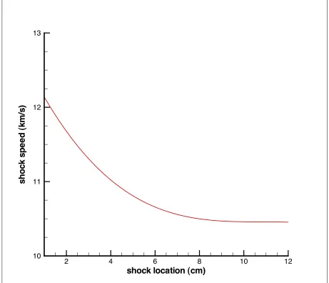
temperature estimate in an iterative process until the computational shock speed matches that of the experiment. However, the shock speed (experimental or computational) is not constant but

rather begins relatively high and drops quickly until its deceleration becomes small and almost

constant. An example of this can be seen in Figure 4.2 Obtaining this situation requires the computational flowfield to be run out for some time. Because of this, the iterative procedure is

listed here is very slow. This process was done only for the nominal shock velocity of 10 km/s.

The temperature found was around 6 000 K for the 0.2 torr case (around 6 000 K to 7 500 K for all cases). These temperatures are much lower than the estimates found using thermodynamic

arguments. This points to problems with shock speed accuracy in DPLR and/or to large losses

when energy is added to the driver gas in experiment. Even with no losses, it is also very possible that the diaphragm ruptures before all the energy is released, resulting in the same issue.

E =mCv∆T (4.1)

Even with access to a parallel computating tool such as DPLR, a solution on a relatively short

mesh (0.5-0.8 m long) took several days on 32-64 processors using the Columbia supercomputer at NASA Ames Research Center (SGI Altix system using 1.6 GHz Intel Itanium 2 Montecito

CPUs). Attempts were made to work around this short mesh limitation by coarsening the grid in

both axial and radial directions or in the axial direction only. However, running such a case to the 7 meters necessary to simulate the actual size of the EAST shock tube caused anomalies in

(22)

trace this computational flowfield to that of the EAST facility.

Initial Conditions

DPLR

mo

dify

Generate Lines-of-Sight

NEQAIR (QSS)

NEQAIR (Boltzmann)

Integrate Integrate

(23)

shock location (cm)

s

h

o

c

k

s

p

e

d

(k

m

/s

)

2 4 6 8 10 12

10 11 12 13

(24)

CHAPTER

5

Results & Discussion

Results shown here consist primarily of spectral radiance or radiance comparisons over various

spectral ranges. Comparisons involving computations, experiments, or both are shown. Not all results involve direct comparision with EAST spectroscopy. For example, comparisons and

discussion involving early CEA results can be found in Bose et al. [2] and are not listed here;

Though the CEA results themselves are listed for comparison with later results. Other comparisons may only involve the differences between different flowfield models, with no concern for experiment.

Still others may show the similarities/differences present in the EAST spectroscopy with no

interest in computation. Dispite this, most comparisions involve both EAST spectroscopy and some sort of computation. These results are divided into several wavelength regions, vacuum

ultraviolet, ultraviolet, visible, near-infrared, and infrared. The intervals involved are completely determined by the EAST spectroscopy, as it is the more limited of the two data sets. The

computational results include both convolved and raw spectral radiance. For the latter, spectral

line shapes and sizes are not directly comparable between computation and experiment. However, it is possible to compare the integral (radiance) over these spectral lines. Midway through this

project, the preferred nomenclature for radiation in the EAST facility changed and the results

here reflect that change. In plots, spectral radiance is referred to both as intensity and as spectral radiance. The integral over wavelength is referred to both as integrated intensity and as radiance.

As the latter set of terms is more widely accepted and the former set is often ambiguous, spectral

(25)

5.1 Nomenclature

In undertaking a discussion of the results obtained through this research, some nomenclature is

used to simplify the description of the workflows/methods used. This nomenclature consists of the flowfield calculation method followed by the radiation calculation method. These two terms will be

hyphenated and appear as a single identifier,e.g. CEA-NEQAIR. Any other pertinent information

is listed in parentheses and follows this identifier. Possible flowfield calculations methods are CEA and DPLR. Possible radiation calculation methods are NEQAIR and NEQAIRup corresponding

to NEQAIR verision 99d and the updated version described here, respectively. Information to

be listed in parentheses includes the addition of impurities into the flowfield and nonstandard options in either the flowfield or radiation calculations. One specified nonstandard option to note

is the use of Boltzmann vs non-Boltzmann (quasi-steady-state) assumptions when modeling the

distribution of excited states in NEQAIR. Unless otherwise noted, a Boltzmann distribution was used.

5.2 Sample EAST Spectroscopy

Experimental data was taken from two test series at the EAST facility. The first of these was

under the direction of Grinstead[7]. The second was under the direction of Cruden[3]. Both

test series used a driven gas tube with an interior diameter of 10.16 cm. The total length of the tube was 8.4 m with spectrographs at about 7 m from the diaphragm rupture point. The driver

gas was Helium while the driven gas contained either synthetic Earth or Martian atmosphere.

Only the Earth atmosphere cases were considered in this work. Data is available for velocities ranging from 9.5 km/s to 10.8 km/s at various driven gas pressures. These velocities and pressures

are representative of some of the typical environments seen by atmospheric entry vehicles at

maximum heating. In both test series, the spectrographs measure spatially (axial only) and spectrally resolved shock-layer radiation as the shock wave passes by windows in the shock tube.

These spectrographs used intensified charged-coupled device (ICCD) cameras to record the data.

The work of Grinstead et al. [7] used two spectrographs to simultaneously capture images in two different wavelength regions during the course of a single shockwave’s passing. The work of

Cruden et al. [3] extended this capability to allow for the use of four spectrographs simultaneously,

greatly improving the amount of useful data obtained from a single test shot. This work and others (Bose et al. [2]) noticed some issues with contamination and baseline radiation in the

data from Grinstead[7]. Because of this, an EAST facility update was undertaken to address

these issues. This was done by the introduction of a shock-tube heater blanket, oil-free vacuum pumps, and most importantly, a oxygen plasma cleaning system for the tube walls. The data

from Cruden[3] includes these updates. Because of contamination issues, this work primarily

(26)

In other to elucidate the results that follow, examples of EAST spectroscopy and its

asso-ciated/derived plots are given. For convenience, the shock structure and EAST camera setup

schematics are repeated here in Figure 5.1 and Figure 5.2, respectively. Almost always, the EAST spectrograph images will include a small portion of region 1 followed by a large portion of

region 2. Occasionally, region 3b will be shown as well. All computational work focuses solely

on region 2. The sample plots here follow the methodology laid out in section 2.1. Begin with the two-dimensional spectrographic image (spectral radiance over axial distance and wavelength).

From this, a radiance profile can be generated against axial distance. This profile is invaluable in

selecting the spatial region over which to average spectral radiance, reducing the two-dimensional image to a single plot of spectral radiance against wavelength.

As mentioned earlier, the experimental flowfield posseses both axial and radial variation, though only the axial is seen directly by spectroscopy. Therefore, a method was devised to

reduce the experimental data so that it could easily be compared with that of computation. This

procedure involves selecting a small axial slice from each spectrographic image and averaging spectra over this portion. Even with almost exactly the same integrated radiance, adjacent axial

(wavelength varying) lines from the spectroscopy can have slightly different spectral radiances.

The averaging within an axial slice is done to reduce the effects of this noise and further reduce the data. Unfortunately, there is no way to remove the effects of radial variation from the experiment.

However, proper selection of the axial slice size and location can be used to reduce the experimental

data as consistently as possible with the assumptions of the computation models. This is done by examining a plot of integrated radiance against axial location for each spectrographic image in

question. Many of these images, as expected, show a spike of radiance at the shock front, followed

by a trough, then a rise and subsequent plateau. A final change in radiance is seen at the location of the contact surface where the driven gas meets the driver gas. In spectrograph images such as

this, it is assumed that the plateau region represents an equilibrium region and this plateau is

taken as the axial slice for data reduction. Unfortunately, not all experimental images follow this expected trend. In these cases, the axial slice is taken to be small and located just forward of the

contact surface. This portion of the flowfield has had the most time to equilibrate and therefore

will be closest to equilibrium. Using this data reduction technique on all the EAST facility spectroscopy allows for simple and direct comparison with the computation spectral radiance

obtained via CEA and NEQAIR or via DPLR and NEQAIR.

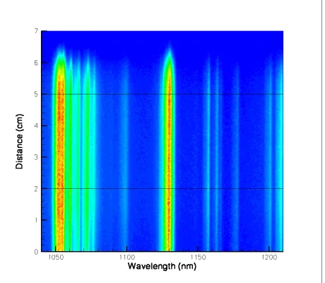
The first example comes from the infrared region of the spectrum. A calibrated spectroscopic image is given by Figure 5.3. The shock front in this image is at approximately 6.5 cm and moving

towards 7 cm. In other words, the datum line for these two example images corresponds to end of the spectrograph’s field-of-view closest to the shocktube diaphragm. It does not, however,

correspond to the actual location of the diaphragm (as the spectrograph is several meters down

(27)

which averaging will be done. To see how these locations were chosen, one needs to look at the

radiance profile given by Figure 5.4. The radiance is found by integrating spectral radiance across

the entire wavelength region captured by the spectrograph. If this is done for each axial location, a radiance profile is obtained. This profile does not show the overshoot in intensity predicted

by theory but could still hold useful radiation data behind the shock front. The region between

2 cm and 5 cm is relatively flat and is chosen to represent region 2 of Figure 5.1. Again, looking at the spectrographic image in Figure 5.3 confirms that this region appears reasonable. Noise

is apparent in both the 2d image and profile, justifying the spatial averaging procedure. The

result of this averaging is given by Figure 5.5. The two-dimensional spectrographic image has been reduced to spectral radiance against wavelength, removing all axial distance dependence

while still representing the region of interest (region 2). This process is repeated for all EAST spectrographic images. All EAST results/comparisons that follow have gone through this process

of data reduction.

The second example comes from the ultraviolet region of the spectrum. The image is given by Figure 5.6. The corresponding radiance profile is given by Figure 5.7. In this profile, the

overshoot predicted by theory is present. The noise is also much higher for this image. This

is due to calibration issues and the smaller wavelength window seen by the spectrograph. The maximum wavelength recorded in this image changes with axial distance. Because of this, a

smaller averaging region (closer to the shockfront) was chosen in order to obtain the largest

wavelength region. The result of averaging between 4 cm and 7 cm is given by Figure 5.8. This is the representative plot for this spectrographic image and is what most, if not all, computational

results are be compared against.

5.3 Updated NEQAIR

The most simple flowfield used in this work is the equilibrium flowfield of CEA. Unfortunately,

discrepancies were found by Bose et al. [2] between these CEA-NEQAIR results and the EAST data of Grinstead et al. [7]. However, samples of these results are still presented here for comparison

with CEA-NEQAIRup calculations. For 0.2 torr and 0.7 torr, the nominal shock speed of 10 km/s

is used and no comparisons with EAST data are visually shown. For 0.3 torr, the experimental shock speed is used and EAST (reduced) spectroscopy is overlayed onto the computational results.

Also, for the 0.3 torr cases, 12% Carbon by mole was added to investigate the effects of impurities.

This percentage was suggested by Bose et al. [2]. All results are convolved with Voigt shapes consistent with the instrumentation of EAST and shown covering wavelength ranges representative

of all spectrograph images in each spectral region.

(28)

CEA. Results for the vacuum ultraviolet, ultraviolet, visible, and infrared spectra are given by

Figure 5.9, Figure 5.10, Figure 5.11, and Figure 5.12, respectively. As mentioned earlier, it was

shown in Bose et al. [2] that 0.2 torr CEA-NEQAIR results matched poorly with EAST facility spectroscopy. These figures are shown solely for the purpose of comparison with updated NEQAIR

results.

Secondly, consider the highest pressure of 0.7 torr. Results for the vacuum ultraviolet, ultraviolet, visible, and infrared spectra are given by Figure 5.13, Figure 5.14, Figure 5.15, and

Figure 5.16, respectively.

Finally, consider the intermediate pressure of 0.3 torr. Results for ultraviolet spectrum are given by Figure 5.17 and Figure 5.18. Results for the visible, near-infrared, and infrared spectra

are given by Figure 5.19, Figure 5.20, and Figure 5.21, respectively. As mentioned earlier, the results for 0.3 torr were obtained by using the experimental shock speed instead of the nominal

shock speed as input to CEA. The effects of this can be seen in the differences between Figure 5.17

and Figure 5.18. CEA-NEQAIR results transition from underprediction to overprediction as wavelength increases from the ultraviolet to the visible spectrum. Some agreement may be

fortuitious, due only to high baseline radiation in EAST not present in NEQAIR.

The first attempt to improve the agreement between computation and experiment involved updating NEQAIR[10]. Firstly, the NEQAIR atomic bound-bound transition database (for C, N,

O) was updated to contain all lines in the NIST Atomic Spectra database. Very few lines were

added and their effects are not studied here. Secondly, Stark broadening curve fit expressions were changed for N and O. Thirdly, several new molecular transition bands were added. Both of

these effects are also small and not studied. Finally, atomic bound-free transition cross-sections

were updated to supplant the Gaunt factor method. The new method directly uses tabulated cross-sections from TOPbase. The effect of this new bound-free update can be seen in the results

that follow.

The results for the ultraviolet, visible, near-infrared, and infrared spectra are given by Figure 5.22, Figure 5.23, Figure 5.24, Figure 5.25. At least in these regions, the bound-free update

has almost no effect. Computations were repeated with all NEQAIR updated features present

and again produced no significant effects. The updating of NEQAIR done in this work does very little to explain or solve the discrepencies between computation and experiment that were noted

in Bose et al. [2].

5.4 DPLR

The final attempt to improve the agreement between computation and experiment involved the

(29)

and experiment exist because of the simplifying assumptions made in the modeling of the

computational flowfield. DPLR-NEQAIR results are shown here for 0.2 torr and 0.7 torr cases

with shock velocities of approximately 10 km/s. Two different cases of 0.2 torr are shown, comparisions are made to EAST spectroscopy, and a cursory analysis is done of boundary-layer

effects.

First, consider a 0.2 torr case on a relatively short mesh of 20 cm beyond intial driver/driven gas discontinuity (diaphragm). The shock speed at this point is approximately 10 km/s. The

translational temperature and axial velocity are shown in Figure 5.26 and Figure 5.27, respectively.

Notice the shock-front curvature and viscous effects evident in both figures. The radial axis begins at the centerline of the tube and goes to the viscous/isothermal wall. The axial axis

datum line is the diaphragm location. As the subtle variation of flowfield in both axial and radial directions is difficult to discern on a contour plot, most of the other results that follow will be

over axial distance with radial slices (constant radius) to show radial variation. Such a plot for

translational temperature can be found in Figure 5.28. The theoretical nonequilibrium overshoot is seen as expected. Again, notice the shock-front curvature that can be seen by the location

of the overshoot in different radial slices. Very close to the wall, hot gas remains long after the

shock has passed; while in the interior of the shock tube, the arrival of the cold driver gas can clearly be seen at around 17.75 cm. The vibrational temperature is shown in Figure 5.29. Again,

the boundary-layer temperature is colder than the interior. The hump centered on 16 cm for

the 97% radial slice most likely corresponds to a bulge in the boundary-layer, though the lack of molecules in the post-shock flow make the vibrational temperature a less reliable measure

than others. Axial velocity shown in Figure 5.30 follows expected trends. That is, the velocity is

mostly constant (around 10 km/s) behind the shock except for near the wall. Figure 5.31 and Figure 5.32 shown pressure and density, respectively. These follow, to a degree, the theoretical

results for a ideal inviscid shocktube. The only exceptions to this being, near the wall, and around

an axial distance of 16 cm. For example, in mixture density plot, the shock front and contact surface is clearly visible. The region between 18 cm and 19.25 cm is the region of interest for

radiation calculations and the region modeled previously by CEA. The arrival of the Helium

driver gas can clearly be seen in Figure 5.33. Finally, the effects of chemistry are clearly shown in Figure 5.34. The percentage of the flow that is ionized increases away from the shock-front,

never reaching a plateau. The peak value, directly in front of the contact surface, is around

12%. Interestingly, this trend is reversed in the boundary layer. That is, the flow becomes less ionized away from the shock-front. Looking at the individual chemcial constituents of the flow

may help to elucidate these issues. The profiles for He, N, N+, O, O+, and electrons can be seen in Figure 5.35, Figure 5.36, Figure 5.37, Figure 5.38, Figure 5.39, and Figure 5.40 respectively.

Molecular species exist almost solely in the boundary-layer. Nitrogen ions are mostly responsible

(30)

highly dissociated and highly ionized while the boundary layer contains colder less ionized gas.

A axial slice of the flowfield was halfway between the shock-front and contact surface. This

slice was then mirrored about the centerline to ensure that a line-of-sight could be constructed for NEQAIR which began at one wall, went through the interior of the flow, and then ended at another

wall. In this way, all physically relevant portions of the flowfield can be included in the simulation

(rather than just an interior as modeled by CEA). NEQAIR was run using this flowfield, both with atomic species only and with atomic/molecular species. This was done to indirectly study

the effect of the boundary-layer on calculated radiance (as most molecules exist in the boundary

layer) in hopes to understand this in the experimental data. The results are given by 5.41(a), 5.42(a), 5.43(a), and 5.44(a). These can be compared with reduced EAST data given by 5.41(b),

5.42(b), 5.43(b), and 5.44(b). The computational results are not convolved, so comparisons should only be done with radiance (not spectral radiance). Almost no difference between atomic only

and atomic/molecular is seen in the vacuum ultraviolet spectrum. However, molecular species

contribute much in the ultraviolet spectrum while they cause significant absorption in the visible and infrared spectra. This could explain some overprediction in high wavelengths when using

CEA-NEQAIR as this boundary-layer effect is not modeled. In the vacuum ultraviolet spectrum,

the primary reason for disagreement is the size of the atomic line at around 1 740 ˚A. In the ultraviolet spectrum, the agreement is relatively good, with the majority of the differences due to

2 000 ˚A to 3 500 ˚A. For the visible spectrum, the differences are due to the high baseline in the

EAST spectroscopy. Notice that the NEQAIR radiance has has flat regions while EAST radiance is always rising due to the baseline. Also, note that the NEQAIR atomic and molecular case fits

much better with the EAST data than the atomic-only case. This can be seen especially well

by looking at the rise in radiance across the lines at 7 500 ˚A and 8 200 ˚A. These rises are much smaller than those seen in the atomic-only case and are consistent with EAST. This alone gives

credence to the importance of the boundary layer in these cases. The disagreement in the infrared

spectrum is due to the relative high strength of several NEQAIR lines. The features at 9 050 ˚A and 9 500 ˚A are much much stronger in NEQAIR than in EAST. Again, these observations are

consistent with the trend of agreement discussed earlier for CEA-NEQAIR. NEQAIR transitions

from underprediction to overprediction as wavelength increases. The use of DPLR has improved this agreement but the trend still exists.

Next, consider another 0.2 torr DPLR case. This case was produced on a longer mesh with a

different CFL schedule and a snapshot at 10 km/s can be seen in Figure 5.47. The features in this flowfield are very similar to those in the previous. The translational and vibrational temperature

profiles are qualitatively and quantitatively similar. This is shown in Figure 5.45 and Figure 5.46. However, the shock-front curvature is reduced significantly. Again, an axial slice of the flowfield

was chosen halfway between the shock-front and contact surface. This was used as input to

(31)

compared directly to EAST data. Results for the ultraviolet, visible, and infrared sectra are given

by Figure 5.50, Figure 5.51, and Figure 5.52, respectively. Again, these can be compared with the

reduced EAST data. However, it is important to note that these figures do not have the same size wavelength interval. Being as these are convolved results, we can compare spectral radiance and

features directly. In the ultraviolet spectrum, the bands at 3 500 ˚A and 3 800 ˚A match between

NEQAIR and EASt. However, the NEQAIR feature at 4 200 ˚A is much weaker in EAST and the EAST features between 2 000 ˚A and 3 000 ˚A are missing from NEQAIR. Again, for the visible

spectrum differences are primarily due to the EAST baseline. Finally, in the infrared spectrum,

NEQAIR relative spectral radiance between lines do not match those in EAST. This points to a difference in distribution of excited states for computation versus reality.

5.5 Conclusions

This work was done in attempts to close the gap between computation and experiment, and to

explain discrepancies seen between these. All comparisons were made against EAST spectroscopy

and all radiation computations done using NEQAIR. Workflows were developed to link CEA or DPLR flowfields to NEQAIR radiation calculations. Several updates were made to NEQAIR

including atomic lines, Stark broadening, bound-free cross-sections, and new molecular bands. It

was found that these updates did little to resolve discrepancies with the EAST facility. Finally, DPLR was used to provide a high fidelity flowfield simulating both axial and radial variation in a

shock-tube. This flowfield, linked with NEQAIR, was used to try to improve or at least explain

the discrepancies between computation and experiment. Some improvement was found though the trends of disagreement discovered with CEA still apply. NEQAIR underpredicts in the ultraviolet

spectrum and overpredicts in the infrared spectrum. The DPLR method could prove promising in the study of the boundary layer in EAST and how its presence affects experimental spectroscopy.

Overall, major discrepancies still remain between NEQAIR computations and EAST spectroscopy.

More study will be required to determine the validity and source of these differences.

1

2 3b

3a

4

x r,y Centerline

(32)

1

2 3b

3a

4 Top View

Spectro-graph

x r,y

Centerline

(33)

(34)

(35)

(36)

(37)

Distance (cm)

In

te

n

s

it

y

(W

/c

m

3

-m

ic

ro

n

-s

r)

0 2 4 6 8 10

0 1 2 3 4 5

(38)

Wavelength (Angstroms)

In

te

n

s

it

y

(W

/c

m

2

-m

ic

ro

n

-s

r)

22000 2400 2600 2800 3000 3200 3400 3600

15 30 45 60 75

(39)

(40)

(41)

(42)

(43)

(44)

(45)

(46)

(47)

Figure 5.17: Comparison of Spectral Radiance from EAST, CEA-NEQAIR, and CEA-NEQAIR

(48)

(49)

(50)

(51)

(52)

Figure 5.22: Comparison of Spectral Radiance from EAST, CEA-NEQAIR, and CEA-NEQAIRup

(53)

(54)

(55)

(56)

Figure 5.26: Translational Temperature Snapshot of DPLR Flowfield showing Shock-Front

(57)

Figure 5.27: Axial Velocity Snapshot of DPLR Flowfield showing Shock-Front Curvature and

(58)

axial (cm)

T

(K

)

15 16 17 18 19 20

0 5000 10000 15000 20000

r/R = 99.6% r/R = 97.0% r/R = 50.0% r/R = 0.0%

Figure 5.28: Translational Temperature Snapshot of DPLR Flowfield showing both Axial and

(59)

axial (cm)

T

v

ib

(K

)

15 16 17 18 19 2

0 2000 4000 6000 8000 10000 12000

r/R = 99.6% r/R = 97.0% r/R = 50.0% r/R = 0.0%

Figure 5.29: Vibrational Temperature Snapshot of DPLR Flowfield showing both Axial and

(60)

axial (cm)

a

x

ia

l

v

e

lo

c

it

y

(m

/s

)

15 16 17 18 19 20

0 2000 4000 6000 8000 10000 12000

r/R = 99.6% r/R = 97.0% r/R = 50.0% r/R = 0.0%

(61)

axial (cm)

P

re

s

u

re

(k

P

a

)

15 16 17 18 19 2

0 5 10 15 20 25 30 35

r/R = 99.6% r/R = 97.0% r/R = 50.0% r/R = 0.0%

(62)

axial (cm)

d

e

n

s

it

y

(k

g

/m

3

)

15 16 17 18 19 20

0 0.01 0.02 0.03

r/R = 99.6% r/R = 97.0% r/R = 50.0% r/R = 0.0%

(63)

axial (cm)

H

e

d

e

n

s

it

y

(k

g

/m

3

)

15 16 17 18 19 2

0 0.005 0.01 0.015 0.02 0.025 0.03

r/R = 99.6% r/R = 97.0% r/R = 50.0% r/R = 0.0%

(64)

axial (cm)

D

e

g

re

e

o

f

Io

n

iz

a

ti

o

n

15 16 17 18 19 20

0 0.02 0.04 0.06 0.08 0.1 0.12

r/R = 99.6% r/R = 97.0% r/R = 50.0% r/R = 0.0%

Figure 5.34: Degree of Ionization Snapshot of DPLR Flowfield showing both Axial and Radial

(65)

axial (cm)

H

e

M

o

le

F

ra

c

ti

o

n

15 16 17 18 19 20

0 0.2 0.4 0.6 0.8 1

r/R = 99.6% r/R = 97.0% r/R = 50.0% r/R = 0.0%

Figure 5.35: Helium Mole Fraction Snapshot of DPLR Flowfield showing both Axial and Radial

(66)

axial (cm)

N

M

o

le

F

ra

c

ti

o

n

15 16 17 18 19 20

0 0.1 0.2 0.3 0.4 0.5 0.6 0.7

r/R = 99.6% r/R = 97.0% r/R = 50.0% r/R = 0.0%

Figure 5.36: Atomic Nitrogen Mole Fraction Snapshot of DPLR Flowfield showing both Axial

(67)

axial (cm)

N

+

M

o

le

F

ra

c

ti

o

n

15 16 17 18 19 2

0 0.02 0.04 0.06 0.08 0.1

r/R = 99.6% r/R = 97.0% r/R = 50.0% r/R = 0.0%

Figure 5.37: Atomic Nitrogen Ion Mole Fraction Snapshot of DPLR Flowfield showing both Axial

(68)

axial (cm)

O

M

o

le

F

ra

c

ti

o

n

15 16 17 18 19 2

0 0.05 0.1 0.15 0.2

r/R = 99.6% r/R = 97.0% r/R = 50.0% r/R = 0.0%

Figure 5.38: Atomic Oxygen Mole Fraction Snapshot of DPLR Flowfield showing both Axial and

(69)

axial (cm)

O

+

M

o

le

F

ra

c

ti

o

n

15 16 17 18 19 20

0 0.005 0.01 0.015 0.02

r/R = 99.6% r/R = 97.0% r/R = 50.0% r/R = 0.0%

Figure 5.39: Atomic Oxygen Ion Mole Fraction Snapshot of DPLR Flowfield showing both Axial

(70)

axial (cm)

E

le

c

tr

o

n

M

o

le

F

ra

c

ti

o

n

15 16 17 18 19 2

0 0.02 0.04 0.06 0.08 0.1 0.12

r/R = 99.6% r/R = 97.0% r/R = 50.0% r/R = 0.0%

Figure 5.40: Electron Mole Fraction Snapshot of DPLR Flowfield showing both Axial and Radial

(71)

Wavelength [Angstroms] Sp e c tr a l R a d ia n c e [W /c m 2 -m i-s r] Ra d ia n c e [W /c m 2 -s r]

1700 1800 1900 2000 2100 0 100 200 300 400 500 0 0.5 1 1.5 2 2.5 3 Atomic

Atomic & Molecular

(a) DPLR-NEQAIR Wavelength [Angstroms] Sp e c tr a l R a d ia n c e [W /c m 2 -m i-s r] Ra d ia n c e [W /c m 2 -s r]

1700 1800 1900 2000 2100 0 500 1000 1500 0 1 2 3 (b) EAST

Figure 5.41: Effect of Boundary-Layer Molecular Species on Spectral Radiance in the Vacuum

(72)

2000 2500 3000 3500 4000 4500 0 50 100 150 200 250 300 0 0.5 1 1.5 2 2.5 3 Atomic

2000 2500 3000 3500 4000 4500 0 20 40 60 80 100 0 0.5 1 1.5 2 2.5 3 (b) EAST

Figure 5.42: Effect of Boundary-Layer Molecular Species on Spectral Radiance in the Ultraviolet

(73)

5000 6000 7000 8000 9000 0 200 400 600 800 1000 0 2 4 6 8 10 Atomic

50000 6000 7000 8000 9000

50 100 150 200 250 300 350 0 2 4 6 8 10 (b) EAST

Figure 5.43: Effect of Boundary-Layer Molecular Species on Spectral Radiance in the Visible

(74)

90000 9500 10000 10500 11000

200 400 600 800 1000 0 1 2 3 4 5 6 7 Atomic

90000 9500 10000 10500 11000

50 100 150 0 1 2 3 4 5 6 7 (b) EAST

Figure 5.44: Effect of Boundary-Layer Molecular Species on Spectral Radiance in the Infrared