ABSTRACT
LI, WEI. Bayesian Inference about Some Geometric Aspects of Nonparametric Functions. (Under the direction of Subhashis Ghosal).
Nonparametric statistics have long been focusing on estimation and inference of some
un-known smooth function f itself. However, some geometric features of the function are also of
great interest in many applications, such as the level curve {x : f(x) = c} or the level set
{x :f(x)≥c} and the filaments of functions. A filament, also called “ridge”, consists of local
maximizers off when moving in a certain direction. Intuitively speaking, the objects of interest
in these problems are sets of points, collectively forming some lower dimensional features of the
function.
The L∞-convergence rates of some smooth multivariate function f are useful for
under-standing the statistical properties of the estimation of level sets{x:f(x) =c}. In the Bayesian
framework, we derive newL∞-posterior contraction rates for multivariate nonparametric
func-tion estimafunc-tion in several different settings. For the multivariate Gaussian white noise model,
theL∞-contraction rates for the functions using trigonometric series and wavelet series priors
are separately derived. Since the collection of level sets for the square root of a nonnegative function coincides with that of the original function, the results based on the square roots of the
functions can lead to useful results for level sets. For binary regression, Poisson regression and
density estimation, the L∞-contraction rates for the square roots of the mean functions and
the square root of the density function respectively, along with their derivatives are obtained.
For these three examples, we use random B-spline series prior and the properties of B-splines
functions to obtain the L∞-rates from the L2-rates through a relaxation argument. All these
L∞-rates yield the contraction rates for level sets in the Hausdorff distance and the Lebesgue
measure of the symmetric difference. In addition, we study frequentist coverage properties of
suitable credible regions for the level sets in both Gaussian white noise model using trigono-metric basis prior and multivariate Gaussian nonparatrigono-metric regression using B-splines basis
prior. A simulation study shows that the credible regions proposed have sufficient frequentist
coverage.
On filament estimation, there have been some recent theoretical studies in the context
of nonparametric kernel density estimation. Our study of filaments contribute to the current literature in two ways. First, we provide a Bayesian approach to filament estimation in the
mul-tivariate nonparametric normal regression context and study posterior contraction rates using
a finite random series of B-splines basis. Compared with the kernel-estimation method, this has theoretical advantage as the bias can be better controlled when the function is smoother, which
of order α ≥ 4, with the optimal choice of smoothing parameters, the posterior contraction rates for the filament points on some appropriately defined integral curves and for the
Haus-dorff distance of the filament are both (n/logn)(2−α)/(2(1+α)). Second, we provide a method
to construct a credible set with sufficient frequentist coverage for the filaments. We study the
© Copyright 2018 by Wei Li
Bayesian Inference about Some Geometric Aspects of Nonparametric Functions
by Wei Li
A dissertation submitted to the Graduate Faculty of North Carolina State University
in partial fulfillment of the requirements for the Degree of
Doctor of Philosophy
Statistics
Raleigh, North Carolina
2018
APPROVED BY:
Anastasios Tsiatis Rui Song
Brian Reich Subhashis Ghosal
BIOGRAPHY
The author was born in Guangzhou, China. Upon completion of his Bachelor’s degree from Capital University of Economics and Business in July 2007, he studied Economics at George
Mason University, and later at Indiana University Bloomington. He completed a Master’s degree in Mathematics and achieved his Ph.D. candidacy in Economics at Indiana University
Bloom-ington before he started pursuing his Ph.D. in Statistics at North Carolina State University in
ACKNOWLEDGEMENTS
First and foremost, I would like to offer my deepest gratitude to my advisor, Professor Subhashis Ghosal, for introducing me to the wonderful world of Bayesian nonparametrics and for his
invaluable advice and guidance that made this work possible. It is a great privilege and fortune for me to share not only of his exceptional scientific knowledge, but also of his extraordinary
professional qualities.
I would also like to thank the rest of my dissertation committee members Professor Anas-tasios Tsiatis, Professor Rui Song and Professor Brian Reich for their valuable suggestions
and encouragement during my research. I would also like to thank Professor Meng Li who is
an Assistant Professor at Rice University for sharing his insight regarding a problem I study in Chapter 4. I am grateful to Professors Dennis Boos, Marie Davidian, Len Stefanski and
Anastasios Tsiatis for the excellent courses they taught.
This work would not be possible without broad inputs from Professors Anastasios Tsiatis, Len Stefanski, Rui Song, Sujit Ghosh, Howard Bondell and Yichao Wu at the early stage
of my Ph.D. study. I have been benefited greatly from their tremendous intellectual insights
which broadens my knowledge of statistics. I thank them for introducing me to their research specialties and their time and patience in problem discussions with me. I am also indebted
to other faculty and staff members in the Department of Statistics at North Carolina State
University for their enthusiastic teachings and assistance.
All my work was also enriched by the Raleigh Chinese Christian Church. During the past
three years, I have been extremely fortunate to be blessed with the love and care from a group
of wonderful fellows in the Agape Bible Study Group and the student fellowship of the Raleigh Chinese Christian Church. I would also like to offer my deep appreciation for them.
Last but not least, I would like to thank my parents, mother-in-law, my daughter and
TABLE OF CONTENTS
List of Figures . . . vi
Chapter 1 Introduction . . . 1
1.1 Bayesian nonparametrics . . . 1
1.2 Posterior contraction . . . 3
1.3 Credible regions and coverage . . . 6
1.4 Research questions and contributions . . . 8
1.5 Notations and preliminaries . . . 9
1.5.1 Notations . . . 9
1.5.2 Trigonometric basis . . . 10
1.5.3 B-Splines Basis . . . 11
1.5.4 Wavelet basis . . . 13
1.6 Roadmap . . . 17
1.6.1 Chapter 2 . . . 17
1.6.2 Chapter 3 . . . 17
1.6.3 Chapter 4 . . . 17
1.6.4 Appendices . . . 17
Chapter 2 Posterior Contraction and Credible Regions for Level Sets . . . 18
2.1 Introduction . . . 18
2.2 Preliminaries . . . 19
2.3 Applications in various inference problems . . . 21
2.3.1 Gaussian white noise model . . . 22
2.3.2 Gaussian regression . . . 24
2.3.3 Binary regression . . . 26
2.3.4 Poisson regression . . . 27
2.3.5 Density estimation . . . 28
2.3.6 Credible sets . . . 29
2.4 Simulation . . . 31
2.4.1 Poisson regression . . . 32
2.4.2 Nonparametric regression . . . 34
2.5 Technical Proofs . . . 37
2.5.1 Proofs of the results for the Gaussian white noise model . . . 37
2.5.2 Proofs of the results for binary regression, Poisson regression and density estimation . . . 43
2.5.3 Proofs of the results for credible sets . . . 51
Chapter 3 Posterior Contraction and Credible Regions for Filaments of Re-gression Functions . . . 55
3.1 Introduction . . . 55
3.2 Preliminaries . . . 57
3.4 Assumptions . . . 59
3.5 Posterior contraction and credible sets for filaments . . . 61
3.6 Simulation . . . 65
3.7 Application . . . 68
3.8 Technical Proofs . . . 70
3.8.1 Some lemmas . . . 70
3.8.2 Proofs of the main results . . . 73
Chapter 4 Direct Bayesian Learning of Level Curves . . . 89
4.1 Introduction . . . 89
4.2 Model, prior and posterior . . . 89
4.3 Discussion . . . 92
4.4 Simulation . . . 93
4.5 Future research . . . 94
References. . . .100
Appendices . . . .108
Appendix A Some auxiliary lemmas . . . 109
LIST OF FIGURES
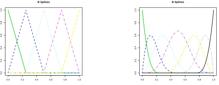
Figure 1.1 B-spline functions. Left plot: q= 2, N = 3. Right plot: q= 4, N = 3. . . . 12
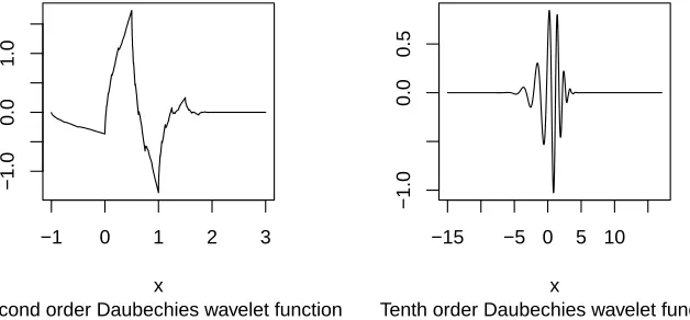
Figure 1.2 Examples of some Daubechies scaling functions and wavelet functions. . . 15
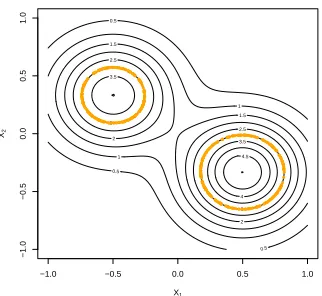
Figure 2.1 The contour of mean function f and true level curve (orange curve). . . . 32
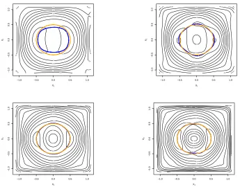
Figure 2.2 Poisson regression √f =bTθ(effects of the smoothing parameter J1 and
J2). The orange circle is the truth, blue curve is estimated level curve
induced by posterior mean. Top left:J1=J2= 6; top right:J1 = 8, J2 =
6; bottom left: J1=J2= 10; bottom right: J1=J2= 12. . . 33
Figure 2.3 Poisson regression f = bTθ (effects of the smoothing parameter J1 and
J2). The orange circle is the truth, the blue curve is the estimated level
curve induced by posterior mean. Top left: J1 =J2 = 6; top right: J1 =
7, J2 = 8; bottom left:J1 =J2 = 10; bottom right:J1 =J2 = 12. . . 34
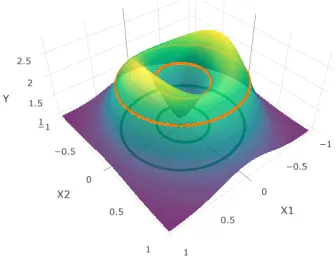
Figure 2.4 The function f and its level curves. . . 35
Figure 2.5 Level curves of a nonparametric regression function (effects of the
smooth-ing parameter J1 and J2). The orange circle is the truth, the blue curve
is the estimated level curve induced by the posterior mean. Top left:
J1 =J2 = 7; top right:J1 =J2 = 9; bottom left: J1 =J2 = 11; bottom
right: J1=J2= 15. . . 36
Figure 2.6 Level curves of a nonparametric regression function (uncertainty
Quan-tification). Left: J1 =J2 = 7. Right:J1 =J2 = 9. . . 36
Figure 3.1 An example of filament curve. . . 56
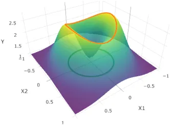
Figure 3.2 The function f and its filament. . . 66
Figure 3.3 Filaments of a nonparametric regression function (effects of the smoothing
parameterJ1 andJ2). The orange circle is the truth, the blue curve is the
estimated filament induced by the posterior mean. Top left: J1=J2= 7;
top right:J1 =J2 = 8; bottom left:J1 =J2 = 9; bottom right:J1 =J2 =
15. . . 67
Figure 3.4 Filaments of a nonparametric regression function (uncertainty
Quantifi-cation). Left: J1 =J2 = 7. Right:J1 =J2 = 9. . . 68
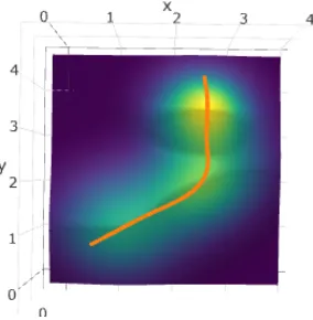
Figure 3.5 Left: Earthquake data points (in red). Right: 100 filaments in the posterior
constructed with high frequentist coverage. The thick blue curves are the filaments induced by the posterior mean. . . 69
Figure 3.6 The magnitude surface and filaments induced by the posterior mean. . . 69
Figure 4.1 The left figure gives the true level curve and the red and blue dots indicate
the directions of the elements ofy. The right figure gives the initial curve
and the red and blue dots indicate the initial directions of the elements
of µ. . . 94
Figure 4.2 Direct Bayes estimate of level curves (0 = 0.5). Going from the left to
the right and from the top to the bottom, these figures show the status in the 100-th, 200-th, 300-th, 400-th, 1000-th iteration and the posterior
Figure 4.3 Direct Bayes estimate of level curves (0 = 1). Going from the left to the right and from the top to the bottom, these figures show the status in the 100-th, 200-th, 300-th, 400-th, 1000-th iteration and the posterior mean with one fifth burn-in. . . 98
Figure 4.4 Direct Bayes estimate of level curves (0 = 5). Going from the left to the
Chapter 1
Introduction
1.1
Bayesian nonparametrics
Nonparametric and semiparametric models are powerful tools in modern statistics. These mod-els assume that some or all parameters involved are of infinite dimensions. In contrast,
para-metric models requires parameters belong to certain subset of Euclidean space (hence a finite
dimensional space). It is well known that parametric models are prone to misspecification in many applications. Nonparametric and semiparametric models offer protection against
mis-specification of all or some components of the models thus allowing for much more flexibility.
However, this flexibility may lead to lower than root-n convergence rates for fully nonparametric components in nonparametric or semiparametric problems. The study of convergence rates for
various nonparametric models in statistics is a very important topic. In the Bayesian paradigm,
we study the posterior contraction rates for certain geometric aspects of some smooth functions and also study the uncertainty quantification for these objects. We shall first present a literature
review and discuss some of the related concepts and issues in Chapter 1.
Bayesian nonparametrics have been attracting wide interests over the past forty years since
the publication of Ferguson (1973). This landmark paper proposed the Dircihlet process, a prior
on spaces of probability measures. After that, many priors have been proposed and studied,
including many kinds of variants of Dirichlet process, Gaussian process, P´olya tree process,
independent increment process and random series prior. Like the convergence of estimators in
the frequentist sense, posterior contraction is an important concept for Bayesian approach. It is essentially about the concentration of the posterior mass around the truth as sample size
increases (see Section 1.2 for more discussion). The general theory of posterior contraction
rates in Bayesian nonparametric models was developed in Ghosal, Ghosh and Van Der Vaart (2000) and Ghosal and Van Der Vaart (2007), respectively for i.i.d (independent and identically
development, readers are referred to Ghosal and van der Vaart (2017). The issues of adaptive
Bayesian estimation were studied in Ghosal, Lember and Van Der Vaart (2003) and Ghosal, Lember and Van Der Vaart (2008) for density functions, Belitser and Ghosal (2003) for the
white noise model in sequence space, and in De Jonge and Van Zanten (2012), Rivoirard and
Rousseau (2012) and Shen and Ghosal (2015, 2016) for some classical models using random
series priors in the Hellinger metric. Knapik, Szab´o, van der Vaart and van Zanten (2016)
studied adaptive estimation in inverse problems for the white noise model. Yoo, Rousseau and
Rivoirard (2018) studied adaptive supremum norm posterior contraction in the multivariate nonparametric regression based on spike-and-slab prior.
The theory of assessing the accuracy of an estimate by confidence statement is of
fundamen-tal importance in statistics. The Bayesian approach has a unique advantage in that the whole inference can be carried out using the posterior distribution alone. One can construct a credible
set which is a region that the parameter will fall onto with certain posterior probability. A
per-haps more interesting question one may ask is whether credible sets can have the right coverage in the frequentist sense. There have been many studies on this important subject recently. The
literature in this direction includes the following papers. Szab´o, van der Vaart and van
Zan-ten (2015) studied adaptive credible regions in Gaussian white noise model. Yoo and Ghosal (2016) addressed similar issues in the multivariate nonparametric regression setting but known
smoothness condition. Knapik, van der Vaart and van Zanten (2011) studied the frequentist coverage of credible sets in nonparametric inverse problems. Belitser (2017) studied credible sets
in mildly ill-posed inverse signal-in-white-noise model. Belitser and Nurushev (2015) studied
uncertainty quantification for the unknown, possibly sparse, signal in general signal with noise
models. van der Pas, Szab´o and van der Vaart (2017) studied credible sets using the horseshoe
prior in the sparse multivariate normal means model in an adaptive setting. Ray (2017) studied
Bernstein–von Mises theorems for adaptive nonparametric Bayesian procedures in the Gaussian white noise model. Yoo and Ghosal (2017) studied Bayesian mode and maximum estimation
and provided credible sets with good coverage. Belitser and Ghoshal (2018) studied uncertainty
quantification for high dimensional linear regression models and their results are also extended to high dimensional additive nonparametric regression models. Using credible regions with
suf-ficiently frequentist coverage, one can obtain confidence regions for the truth in the frequentist
sense relatively easily from the posterior distribution. This is especially appealing when the object to be studied is complicated. For instance, the level set or the filament of functions, or
other geometric aspects of functions. See Section 1.3 for more discussion on credible sets.
f :Rd→Rin some regular space (for instance,L2),f can be expanded as
f = ∞
X
j=1
fjψj,
for some suitable basis functions ψ = {ψ1, ψ2, . . . .}, where fj may be considered as some
generalized Fourier coefficient. This expression has infinitely many terms, while in the model
one can express f asf =PJ
j=1θjψJ,j,ψJ ={ψJ,1, ψJ,2, . . . , ψJ,J} for some J going to infinity
as sample size increases. For a multivariate problem (d >1), the basisψJ is often constructed
as tensor-product of bases along each dimension. It should be understood for the multivariate
case, that the total number of termsJ in the expansion should then be viewed as the product of
the number of terms in each dimension. With this series representation, the estimation problem
can be viewed as estimating θ = (θ1, . . . , θJ), or equivalently, estimating f from the space
F(J) = {PJ
j=1αjfj :αj ∈R}. This truncated version of estimator is useful when it has good
approximation property. That is, for some sufficiently largeJ,
inf
f∞∈F(J)kf−f
∞k∞
.J−α/d. (1.1)
The coefficient α is normally some smoothness coefficient for the functionf. Many choices of
bases are available that have this approximation property. We shall discuss with the
trigonomet-ric basis, B-spline basis and wavelet basis. For more treatment on approximation of functions,
see DeVore and Lorentz (1993); Lorentz (2005); Powell (1981).
When a density function p is of interest, it can be modeled as
p:= R Ψ(f)
Ψ(f)dµ,
for some positive link function Ψ andf =PJ
j=1θjψj. A common choice for Ψ is the exponential
function. Modeling p = PJ
j=1θjψj is also possible, provided that R PJj=1θjψj = 1 for any J
and ψj ≥0.
1.2
Posterior contraction
In this section, we shall briefly discuss the theory of posterior contraction. Suppose one has
ob-servationsX = (Xi)ni=1whose joint distribution is given byPf(n)with the corresponding density
functionp(fn). When the observations are independent (not necessarily identically distributed),
we write Pf(n) = Nn
i Pfi and p
(n)
f =
Qn
i pfi, where fi denotes f(Xi). Here f belongs to some
f. Let Πn(·|X) denote the corresponding posterior defined by
Π(B|X) =
R
Bp
(n)
f (X)dΠ(f)
R
p(fn)(X)dΠ(f)
. (1.2)
The posterior distribution Πn(·|X) is said to be consistent at the truth f∗ ∈ F if for any
>0,
Πn(θ:dn(f, f∗)> |X)→0, (1.3)
inPf(n∗)-probability asn→ ∞.
We say that a sequence n is a posterior contraction rate at the parameterf∗ with respect
todnif for anyKn→ ∞,
Πn(θ:dn(f, f∗)> Knn|X)→0, (1.4)
in Pf(n∗)-probability as n → ∞. The smallest n that satisfies this definition is of particular
interest, as it gives us the fastest possible rate. In many classical examples, one would hope
that this rate is equal to or close to the “optimal” frequentist rate.
Posterior contraction essentially guarantees that the information in the data can override
the prior opinions as the sample size increases. From a subjective Bayesian’s point of view,
consistency can also be equivalently interpreted as the merging of predictive distributions of future observations—another desired property. Posterior contraction can also provide point
estimators (for many cases, posterior mean) that converge at the same rate .
As mentioned previously, the general theory of posterior contraction rates in Bayesian non-parametric models was developed in Ghosal et al. (2000) and Ghosal and Van Der Vaart (2007),
respectively for i.i.d (independent and identically distributed) observations and general
obser-vations. In this general theory, the existence of tests of exponentially decaying errors plays a fundamental role. On the other hand, Shen and Wasserman (2001) also studied posterior
con-traction rates for i.i.d. observations but using different and stronger conditions. These works
focused on consistency and contraction rates in the Hellinger metric.
Let the Hellinger distance betweenpandqbe defined as (R
(√p−√q)2dµ)1/2. The
Kullback-Leibler divergence (KL divergence) is defined byK(p, q) =R plog(p/q)dµ. The master theorem
in general can give rates for the Hellinger distance on the densities induced byf. We may
inter-pretdn(f1, f2) asdH(pf1, pf2) when the data are i.i.d, or asdH,n:=
q
Pn
i=1d2H(pf1,i, pf2,i)/n, the
root-average squared Hellinger distance when the data are independently (but not identically) distributed.
The book Ghosal and van der Vaart (2017) has in-depth discussion on general theory. We
shall present some of these results.
test φn such that
Pf(n∗)φn→0, sup
f∈Fn:dn(f,f∗)>n
Pf(n)(1−φn)≤exp(−Cn2n), (1.5)
and that for some constantL >0 and some sufficiently large constant b >0,
Πn(f ∈ Fn:K(p(fn∗), p
(n)
f )≤n
2
n)≥exp(−Ln2n),
Πn(F \Fn)≤exp(−bn2n),
thenΠ(dn(f, f∗)> Knn|Y)→0, for every Kn→ ∞.
Condition (1.5) requires the existence of a test whose type I error probability tends to zero and
type II error probability is exponentially decaying on the space Fn. We shall give a sufficient
condition for (1.5). To this end, we need the concept of covering number. Given a metric or
semimetric space (T, d), for any >0, its covering numberN(T, d, ) is defined as the smallest
number of closed d−balls of radius needed to cover T. A sufficient condition for (1.5) is now
given in the following:
Suppose for two arbitrary semimetricdn, enonF, there exists some constantsC1>0, C2>
0, ξ > 0 so that for every >0 and every f1 ∈ Fn with dn(f1, f∗) > , one can find a test φn with the exponential error probabilities
Pf(n∗)φn≤exp(−C1n2), sup
f∈Fn:en(f,f1)<ξ
Pf(n)(1−φn)≤exp(−C2n2), (1.6)
and that
logN(n,Fn, en).n2n. (1.7)
The condition expressed in (1.6) is the basic testing condition. By the Le Cam–Birg´e testing
theory, it holds for the Hellinger distance (when the observations are i.i.d) and the root-average
squared Hellinger distance (when the observations are independently distributed). The entropy
condition (1.7) requires that one can use a collection of ball-like sets with respect toento cover
Fn and this collection is not too large.
Though above result allows fairly general metric dn, it is not automatically extended to
the Lp-norms (1 ≤ p ≤ ∞), as the Condition (1.6) does not readily hold for these metrics.
The contractions rates in the Lp-norms (1 ≤ p ≤ ∞) were studied in Gin´e and Nickl (2011).
The minimax contraction rates were obtained for density estimates for 1 ≤ p ≤ 2 and for
the Gaussian white noise models using conjugate priors for all 1 ≤ p ≤ ∞. More recently,
leads to the minimax contraction rates in the density estimation with log-density prior and
the Gaussian white noise models with nonconjugate priors. Yoo and Ghosal (2016) established
the optimalL2- and L∞- rates for the regression function and its mixed partial derivative but
with conjugacy. Shen and Ghosal (2017) studied both L2- and L∞- rates for density and its
derivatives. They showed that the minimax rate for theL2- distance is obtained.
Theorem 1.2.1 is a very general one as it does not require any specific type of prior on f.
For finite random series priors, more explicit results can be presented. We summarize some of
those relevant results in Appendix B and shall use them intensively in the proofs of some main results in Chapter 2.
1.3
Credible regions and coverage
Constructing confidence bands in nonparametric problems is a very important topic in itself.
Some recent papers include Claeskens and Van Keilegom (2003), Gin´e and Nickl (2010) and
Chernozhukov, Chetverikov and Kato (2013, 2014a). As discussed earlier, an interesting and important question from Bayesian perspective is to ask whether the credible region can have
good frequentist coverage. We start with a definition. Consider the parameter θ in a finite
dimensional model (Θ⊂Rp). Formally, for some positive value γ ∈(0,1), a subset C(X) of Θ
is called a 1−γ credible region if
Πn(θ:θ∈C(X)|X) = 1−γ.
Let Xi i.∼i.d. Pθ0. According to the celebrated Bernstein-von-Mises Theorem, under some
regu-larity conditions,
√
n(θ−θ˜)|X∼d N(0, I(θ0)−1),
where ˜θ is the posterior mean and I(θ0) is the Fisher information. Since ˜θ is asymptotically
equivalent to a frequentist efficient estimator (say, the MLE), this guarantees that the credible
regionC(X) ={θ:kθ−θ˜k ≤Rγ}, whereRγ is the 1−γ quantile of the posterior distribution
of θ−θ˜, has the right exact asymptotic frequentist coverage. That is,
P(θn)
0 (kθ0−
˜
θk ≤Rγ) = 1−γ.
Unfortunately, in the infinite dimensional model (when Θ =F endowed with distance function
dn on functions), this result may no longer hold (Cox; 1993; Freedman; 1999). However, a
weak functional of Bernstein-von-Mises theorem was put forward in Castillo and Nickl (2014);
Gin´e and Nickl (2010) and the credible region constructed in some weaker norm with exact
A different approach is that, if the requirement of “exact” coverage is relaxed, it is possible
to find an “inflated” credible set C(X) ={θ:dn(θ,θ˜)≤ρnRγ}, for someρn→ ∞ (or possibly
a large fixed constant) such that,
lim inf
n θinf0∈Θ
P(θn)
0
dn(θ0,θ˜)≤ρnRγ
→1, asn→ ∞,
and the posterior quantile Rγ has the same order as the minimax rate of estimating the
pa-rameterθ0—a rate usually can be achieved by the posterior mean ˜θ. A recent paper by Szab´o
et al. (2015) studied adaptive nonparametric regions in the above sense with the full parameter
space Θ replaced by some dense subset in the Gaussian white noise model. Yoo and Ghosal
(2016) addressed similar issues in the multivariate nonparametric regression setting with known smoothness condition. Some other papers are mentioned in the Section 1.1. A credible set with
sufficient but not exact coverage can also be obtained through undersmoothing without using
any inflating factor, but this leads to suboptimal estimation.
To briefly compare the frequentist and Bayesian approaches, we focus on the uniform
un-certainty quantification for the function itself. Letf∗ denote the true function. Suppose Rγ is
the 1−γ quantile of kfˆ−f∗k∞, then
P(kfˆ−f∗k∞≤Rγ) = 1−γ.
Therefore, a valid 1−γ uniform confidence region for f∗ is {g :kg−fˆk∞ ≤ Rγ}. Note that
the uniformity is in the sense that Rγ does not depend on any given point x as in contrast
to the radius in pointwise confidence interval. The difficulty then is the estimation of the
quantilesRγ. For some cases, when asymptotic distribution of thekfˆ−f∗k∞can be derived, the
quantile can be obtained accordingly. As an alternative, to estimate the quantileRγ, bootstrap
can be used and some theoretical foundations are established in Chernozhukov et al. (2013,
2014a) and Chernozhukov, Chetverikov and Kato (2014b). However, it is worth to point out
that in the bootstrap approach, it is the distribution kfˆ−E ˆfk∞ that is approximated by the
bootstrap distribution. Strictly speaking, it is the quantile ofkfˆ−E ˆfk∞ that can be obtained
and confidence region obtained would be for E ˆf instead off∗.
We turn to Bayesian approach. Let ˜f be the posterior mean of f. One can construct the
credible region as {g : kg−f˜k∞ ≤ ρnRγ} for some inflation constant ρn, where here Rγ is
the 1−γ quantile of posterior distribution of kf −f˜k∞. It can be shown that in some cases
this credible set can have sufficient frequentist coverage (Yoo and Ghosal; 2016). Additional
property may be obtained also. For instance, the radius of the region can have the same rate as
the optimal rate of estimatingf∗ in theL∞-norm. To ensure an inflation factor of the correct
estimated; see for instance the proof of the results in Section 2.3.6. The benefit of Bayesian
approach is that the posterior samples are readily available thus finding the right quantile is
easier than the bootstrap procedure. Furthermore, the inferential target is f∗, rather than the
expected value of the estimator.
1.4
Research questions and contributions
The strategy for uncertainty quantification using confidence region or credible region for the
function itself is more or less well understood. In the literature there are some other problems where estimation and inference is performed for a set, or more broadly speaking for some
geometric object (Molchanov; 2006). In this dissertation, we consider two features, level sets
and filaments. A level set of a multivariate functionf is defined as the setL:={x:f(x) =c}or
L:={x:f(x)≥c}. The filament, to avoid technicalities here, can be viewed as a collection of
local maximizers off that behaves like a lower dimensional manifold. The study of estimation
of level sets dates back to 1990’s while that of filaments is more recent. Both of these problems fall into a broad category of data analytic methods known as topological data analysis, which
is used to find structure in data (Wasserman; 2016). Some other examples arise in econometrics
literature where partially identified parameters are the objects of interest (Chernozhukov, Hong and Tamer; 2007; Chernozhukov, Kocatulum and Menzel; 2015).Most papers study estimation
of levels and filaments in the frequentists setting while there are few recent papers on inference.
To our best knowledge, there is only one published Bayesian paper on level set estimation (Gayraud and Rousseau; 2005) and no study on filament using the Bayesian approach.
The L∞-rates of the estimates of functionsf are essential for understanding the statistical
properties of the procedures that estimate level sets and filaments. The idea in the last section on credible region of the function may be used to make inference about level sets and filaments.
Posterior contraction of the functions in sup-distance can induce credible regions on some
features of the functions. This becomes apparent when the Hausdorff distance of level sets or the filaments can be bounded by the sup-distances on the functions or the derivatives of the
functions.
In this dissertation, we address the following issues. First, we derive new L∞-posterior
contraction rates for the multivariate functions in several different nonparametric settings. For
the multivariate Gaussian white noise model, the L∞-contraction rates for the functions using
trigonometric series and wavelet series priors are separately derived. Since the collection of level sets for the square root of a nonnegative function coincides with that of the original function,
the results based on the square roots of the functions can lead to useful results for level sets. For
binary, and Poisson regression and density estimation, theL∞-contraction rates for the square
their derivatives are obtained. For these three examples, we use random B-spline series prior
and the properties of B-splines functions to obtain the L∞-rates from the L2-rates through
a relaxation argument. These rates may not be optimal but they are new in the literature
and should be useful as some intermediate results. Second, as by-products, all these L∞-rates
yield the contraction rates for level sets in the Hausdorff distance and the Lebesgue measure of the symmetric difference. Third, we study frequentist coverage properties of suitable credible
regions for level sets in both Gaussian white noise model using trigonometric basis prior and
multivariate nonparametric normal regression using B-splines basis prior. A simulation study shows that the proposed credible regions have sufficient frequentist coverage.
Our study of filaments contribute to the current literature in two ways. First, we provide a
Bayesian approach to filament estimation in the multivariate nonparametric normal regression context and study the posterior contraction rates using a finite random series of B-splines
basis. Compared with the kernel-estimation method, this has theoretical advantage as the bias
can be better controlled when the function is smoother, which allows obtaining better rates.
Assuming thatf :R2 7→Rbelongs to an isotropic H¨older class of orderα≥4, with the optimal
choice of smoothing parameters, the posterior contraction rates for the filament points on some
appropriately defined integral curves and for the Hausdorff distance of the filament are both
(n/logn)(2−α)/(2(1+α)). Second, we provide a way to construct a credible set with sufficient
frequentist coverage for the filaments. We study the performance of our proposed method by simulations and application to an earthquake dataset.
1.5
Notations and preliminaries
In this section, we shall describe notations and briefly introduce the preliminaries for three common function bases.
1.5.1 Notations
Let N = {1,2, ..,}, N0 = {0,1,2,3, . . .}. Given two real sequences an and bn, an = O(bn) or
an.bnmeans thatan/bnis bounded, whilean=o(bn) oranbnmeans thatan/bn→0.Also
an bn means that both an =O(bn) andbn =O(an). For random element Zn,Zn = Op(an)
means that P(|Zn| ≤Can)→1 for some constant C >0.
For a vectorx∈Rd, we definekxk
p= (Pdk=1|xk|p)1/pfor 0≤p≤ ∞,kxk∞= max1≤k≤d|xk|
and write kxk for kxk2. For an m×m matrix A, let kAk(r,s) = sup{kAxks : kxkr ≤ 1}. In
particular,kAk(2,2) = (λmax(ATA))1/2, whereλmax denotes the largest eigenvalue; kAk(∞,∞)=
max1≤i≤mPmj=1|aij|. Let kAkF =
p
tr(ATA) stands for the Frobenius norm of matrix A. We
For two probability densities f and g, the Lp- distance (1 ≤ p < ∞) is given by (R
|f −
g|pdµ)1/p assuming the σ-finite measure is given by µ. The Hellinger distance between f and
g is defined as (R
(√f−√g)2dµ)1/2. The Kullback-Leibler divergence (KL divergence) is given
by K(f, g) =R
flog(f /g)dµ.
Consider f : U 7→ R defined on some bounded set U ⊂ Rd. For 1 ≤ p < ∞, let kfkp
be the Lp- norm (R
|f|pdν)1/p with respect to some measure ν. For some probability measure
G, let kfkp,G = (
R
|f|pd
G)1/p. The supremum norm is denoted by kfk∞ = supx∈U|f(x)|. For
g:U 7→R1 on some bounded setU ⊂Rd, let ∇g be the gradient ofg, which is a d×1 vector.
For a d-dimensional multindexr = (r1, . . . , rd)∈Nd0, let Dr be the partial derivative operator
∂|r|/∂xr1
1 · · ·∂x
rd
d where|r|=
Pd
k=1rk.
For some integer q≥1, letCq([0,1]d) denote the space ofq-times continuously differentiable
functions on [0,1]d. The H¨older Space Hα([0,1]d) of order α > 0 consists of functions f :
[0,1]d7→R such thatkfkα,∞<∞, wherek · kα,∞ is the H¨older norm
kfkα,∞= max
r:|r|≤bαcsupx
|Drf(x)|+ max
r:|r|=bαcx,ysup:x6=y
|Drf(x)−Drf(y)|
kx−ykα−bαc ,
where sup is taken over the support off andbαc is the largest integer strictly smaller thanα.
We shall also need the Hausdorff distance for our study of level sets and filaments. Given
two sets A and B in Euclidean Space, let d(A|B) := supx∈Ainfy∈Bkx−yk. If A ={x}, write
d(x|B) =d({x}|B) := infy∈Bkx−yk .The Hausdorff distance between Aand B is defined as
Haus(A, B) = max{d(A|B), d(B|A)}. (1.8)
1.5.2 Trigonometric basis
Consider the trigonometric basis on R: φ1 = 1, φ2j =
√
2 cos(2πjx), φ2j+1 =
√
2 sin(2πjx),
j= 1,2, . . .. Functions of period 1 onRor the periodic extension of functionf defined on [0,1] can be expressed as
f =α0+ ∞
X
j=1
[αjcos(2πjx) +βjsin(2πjx)].
Consider a function f : [0,1]d 7→ R. Let j = (j1, . . . , jd) ∈ {0,1,2, . . .}d and K(j) := {k ∈
{0,1}d : k
i = 0 whenji = 0, i = 1, . . . , d}. We denote the tensor product trigonometric basis
functions by{φjk : (j, k)∈ {0,1,2, . . .}d× K(j)}, where
φjk(x) = d
Y
i=1 √
The function f can be written as
f(x) = ∞
X
j1
· · · ∞
X
jd
X
k∈K(j)
φjkθjk.
For brevity, we may simplify the indices of summation and just write f = P
j
P
kφjkθjk.
Consider the space of the form
Fn=Fn,t:=
Jn
X
j1=0
· · ·
Jn
X
jd=0
X
k∈K(j)
αjkφjk :αjk ∈R
.
Iff ∈ Hα([0,1]d), for Jn sufficiently large, one has (Schultz; 1969):
inf
f∞∈F n,t
kf−f∞k∞.Jn−α.
Notice that the order is (Qd
l=1Jn)−α/d as described in the expression (1.1).
1.5.3 B-Splines Basis
Let a sequence of knots {ti : 0 = t0 < · · · < tN+1 = 1} be a partition of the interval [0,1]
into N+ 1 subintervals : Ii = [ti, ti+1) for i= 0, . . . , N−1 and IN = [tN−1, tN]. The space of
(polynomials) splines of orderq defined on [0,1] is a linear space such that
(i) each element f is a polynomial of order at most q on each interval Ii;
(ii) each elementf belongs to Cq−2[0,1].
Intuitively speaking, a spline function is a piecewise polynomial which has global smoothness
over the whole interval. B-splines are one particular basis for the space of splines. Let δi =
ti+1 −ti for i = 0, . . . , N and ∆ = max0≤i≤Nδi. We assume a quasi-uniform knot sequence,
i.e., ∆/min0≤i≤Nδi ≤ C for some constant C > 0. Note that the equidistant knot sequence,
i.e., δi all being all equal, is a special case. To construct this basis, extended knots are required
and we assume they are all positioned at the end points of the interval. We denote the B-spline
functions by {B1,q, . . . , BN+q,q}. These functions can be defined using divided difference or by
the following convenient recursive formula:
Bi,q(x) = x−ti−q
ti−1−ti−q
Bi−1,q−1(x) +
ti−x ti−ti+1−q
Bi,q−1(x), i= 1, . . . , q+N.
By construction, we immediately have Bi,q(x) >0 on (ti−q, ti) and PNi=1+qBi,q = 1. These
functions constitute a linear space of dimension J = q+N. In particular, for any given x ∈
[ti, ti+1), only at mostqadjacent B-spline functions are nonzero: (Bi+1,q, . . . , Bi+q,q). Figure 1.1
gives some examples of B-spline functions.
Consider a linear combination of the B-spline functions given by f =PJ
j=1θjBj,q(x). For
some integerq > s≥1, the derivative ofD(s)f is given byDsf(x) =PJ−s
j=1θ
(s)
j Bj,q−s(x),where
θ(s)= (q−s)θ
(s−1)
j+1 −θ
(s−1)
j tj−tj−q+s
.
LetbJ,q be the column vector of{Bi,q: 1≤i≤J}and θ= (θ1, . . . , θJ)T. It can be shown that
Dsf(x) =bTJ−s,q−sWsθfor some (J−s)×smatrixWsand each nonzero entry ofWs is of order
Js. HerebJ−s,q−s consists of (q−s)-order B-spline functions defined on the same interval using
the same sequence of interior knots.
0.0 0.2 0.4 0.6 0.8 1.0
0.0
0.2
0.4
0.6
0.8
1.0
B Splines
0.0 0.2 0.4 0.6 0.8 1.0
0.0
0.2
0.4
0.6
0.8
1.0
B Splines
Figure 1.1: B-spline functions. Left plot:q = 2, N = 3. Right plot: q= 4, N = 3.
To model a multivariate function f ∈ Hα([0,1]d), we can make use of the tensor product
of B-splines basis. Define bJ1,...,Jd,q1,...,qd(x) = (Bj1,...,jd(x) =
Qd
k=1Bjk,qk(xk) : 1 ≤ jk ≤ Jk)
T
to be a column vector of tensor product of B-splines functions, with possibly different orders
qk and knot sequences in different directions, i.e., 0 = tk,0 < tk,1 <· · · < tk,Nk < tk,Nk+1 = 1
for k = 1, . . . , d; here Nk denotes the number of interior points and Jk = qk +Nk denotes
the number of basis functions on the jth coordinate. The elements of this vector are assumed
to be in the dictionary order according to their indices. Whenever q1, . . . , qd are considered
k = 1, . . . , d, define δk,l = tk,l+1−tk,l forl = 0, . . . , Nk. Let ∆k = max0≤l≤Nkδk,l. We assume
that ∆k/min0≤l≤Nkδk,l ≤Cfor someC >0. This assumption is clearly satisfied for the uniform
partition. Therefore we writef(x) =bT
J1,...,Jd(x)θ, or simplyf(x) =b
T(x)θ. As in the univariate
case, we haveDrf(x) =bJ−r,q−r(x)TWrθ for some
Qd
k=1(Jk−rk)×
Qd
k=1Jk matrix Wr .
Several properties of B-splines are important for our purpose and they are listed as follows:
0≤Bj1,...,jd ≤1 for all 1≤jk≤Jk, k= 1, . . . , d andx∈[0,1]
d;
PJ1
j1=1· · ·
PJd
jd=1Bj1,...,jd(x) = 1 for all x∈[0,1]
d;
Bj1,...,jd is supported on
Qd
k=1[tk,jk−qk, tk,tk).
For the moment, we fix qk > α and let Nk (hence Jk) increase as sample size increases,
for k = 1, . . . , d. Yoo and Ghosal (2016) showed that each nonzero entry of Wr is uniformly
O(Qd
k=1J
rk
k ). Therefore, kWrk∞,∞=O(
Qd
k=1J
rk
k ) and kWrTWrk(2,2) =O(
Qd
k=1J
rk
k ). We also
have the following approximation property. Consider the space of the form
Fn=Fn,b:=
Jn
X
j1=1
· · ·
Jn
X
jd=1
αj1,...,jdBj1,q1(x1)· · ·Bjd,qd(xd) :αj1,...,jd ∈R
.
Iff ∈ Hα([0,1]d) and q
k ≥α fork= 1, . . . , d, forJn sufficiently large, one has
inf
f∞∈F n,b
kf−f∞k∞.Jn−α.
For more treatment of B-splines functions, readers may refer to De Boor (1978) and Schumaker
(2007).
1.5.4 Wavelet basis
There is a rich literature on both theory and applications of wavelets. Our discussion here
is mainly based on H¨ardle, Kerkyacharian, Picard and Tsybakov (2012) and Gin´e and Nickl
(2015).
Definition 1.5.1 A system of real-valued functions {φk :k∈ Z} of L2(R) is an orthonormal
system if hφk, φk0i := R φk(x)φk0(x)dx = 1 if k = k0, and hφk, φk0i = 0 otherwise. It is an
orthonormal basis for a subspaceV of L2(R) if for any functionf ∈V,f(x) =Pkckφk(x) in
L2, with P
|ck|2 <∞.
Let φbe some function from from L2(R) such that:
2. the collection of linear spaces Vl := {h(x) = f(2lx) : f ∈ V0}, l ∈ Z satisfies that
Vl ⊂Vl+1, l∈Zand ∪l≥0Vl is dense inL2(R).
The sequence of spaces {Vl :l ∈Z} is called a multiresolution analysis (MRA) of L2(R). The
collection of dilations and translations {φlk := 2l/2φ(2l· −k) : k ∈ Z} forms an orthonormal
basis for Vl for each l ∈ N. Such a function φ is called the father wavelet or scaling function
that generates this MRA.
If furthermore, for a given MRA, some function ψ can be found such that the collection
{ψlk := 2l/2ψ(2l· −k) : k ∈Z} is an orthonormal basis for the orthogonal complement Wl :=
Vl+1 Vl in Hilbert space for each l ∈ N. Then one can express Vl = V0 ⊕(⊕ll−1=1Wl) and
L2(
R) = V0 ⊕(⊕∞l=1Wl). Here the expression using ⊕ means an orthogonal decomposition in
Hilbert space. That is, the collection of the functions
φk=φ(· −k), ψlk= 2l/2ψ(2l· −k), l∈ {0} ∪N, k∈Z,
forms an orthonormal basis ofL2(R). Therefore, for anyf ∈L2(R), one can write
f =X
k∈Z
hφ0k, fiφ0k+
∞
X
l=0
X
k∈Z
hψlk, fiψlk inL2.
This expansion is called the wavelet expansion. The functionψ is called the mother wavelet or
simply the wavelet. The indexl refers to the resolution level.
The simplest orthogonal wavelet basis is Haar wavelet basis which has scaling function
φ(x) = 1[0,1](x) and wavelet function ψ(x) = 1[0,1/2)(x)−1[1/2,1](x). In fact, Haar wavelet is
a special case of a more general family of wavelet bases called Daubechies wavelets. The most important features of this family are that the (orthogonal) wavelets have compact support in
time domain and can be arbitrarily smooth. To be more precise, for any N ∈ N, Daubechies
wavelet basis of order N can be constructed so that its scaling function and wavelet functions
are at least bλ(N −1)c continuously differentiable for some λ ≥ 0.18 and wavelet functions
have N vanishing moments. Figure 1.2 gives some examples of Daubechies scaling functions
and wavelet functions.
Another interesting variant is the boundary-corrected wavelet basis of Cohen, Daubechies
and Vial (1993), called the CDV-wavelet basis. The coefficients of wavelet expansions in this
sufficiently large resolution level sayJ0. The expansion can be written as
f =
2J0−1
X
k=0
hφJ0k, fiφJ0k+
∞
X
l=J0
2l−1
X
k=0
hψlk, fiψlk.
Regular wavelet bases have rich theoretical properties. It suffices to point out that the above
wavelet expansion does not only converge in L2 but also in L∞, provided that f is uniformly
continuous. Wavelet functions have localization property: kP
kck|ψlk|k∞.maxk|ck|2l/2 for a
sequence of real number{ck:k∈Z}such that maxk|ck|<∞. Whenf isα-times continuously
differentiable, using sufficiently regular wavelet basis, supk∈Z|hf, ψlki|.2−l(α+1/2) for alll≥0.
0.0 1.0 2.0 3.0
0.0
0.5
1.0
Second order Daubechies scaling function x
−1 0 1 2 3
−1.0
0.0
1.0
Second order Daubechies wavelet function x
0 5 10 15
−0.4
0.0
0.4
0.8
Tenth order Daubechies scaling function x
−15 −5 0 5 10
−1.0
0.0
0.5
Tenth order Daubechies wavelet function x
Suppose that φ, ψ are the scaling function and wavelet of a Daubechies wavelet basis of
L2(R). That is, the collection of the functions
φk=φ(· −k), ψlk= 2l/2ψ(2l· −k), l∈ {0} ∪N, k∈Z,
forms an orthonormal basis ofL2(R). We assume thatφ, ψare bothq-times (q > α) continuously
differentiable. A wavelet basis on [0,1]d(called CDV-wavelet basis) can be constructed fromφ, ψ
starting from some sufficiently large fixed resolution levelJ0. We shall use the same notations for
this basis so that{φk, ψlk0 : 0≤k≤2J0−1,0≤k0≤2l−1, l∈N, l≥J0}form an orthonormal
basis forL2([0,1]). LetK(l) ={0, . . . ,2l−1}dandIis the set of sequencei= (i
1, . . . , id) of zeros
and ones excluding i= (0, . . . ,0). Standard theory suggests a wavelet series for f ∈L2([0,1]d)
can be written as
f = X
k∈K(J0)
hf,ΦkiΦk+
∞
X
l=J0
X
i∈I,k∈K(l)
f,Ψil,kΨil,k,
where
Φk(x) : = ΦJ0k(x) =φJ0k1(x1)· · ·φJ0kd(xd),
Ψilk(x) : =ψi1
lk1(x1)· · ·ψ
id
lkd(xd);
here ψ0lk(·) :=φlk(·) = 2l/2φ(2l· −k) andψlk1(·) :=ψlk(·). In the proof, we will mainly use the
following properties of this wavelet basis:
kP
k∈K(J0)|Φk|k∞.2
J0d/2,kP
k∈K(l)|Ψil,k|k∞.2ld/2;
forf ∈ Hα([0,1]d) withα < q, sup
i∈I,k∈K(l)|hf,Ψil,ki|.2
−l(α+d/2) for alll≥0.
Consider the space spanned above tensor wavelet basis
Fn=Fn,w :=
X
k∈K(J0)
αJ0kΦk+
Jn
X
l=J0
X
i∈I,k∈K(l)
βlkΨil,k :αJ0k, βlk∈R
.
Iff ∈ Hα([0,1]d) and wavelet basis is q-regular (q > α), for J
n sufficiently large, one has
inf
f∞∈F n,w
kf−f∞k∞.2−αJn.
Compared with the approximation errors using the trigonometric basis and the B-splines basis,
1.6
Roadmap
1.6.1 Chapter 2
In this chapter, we study theL∞- posterior contraction rates for the nonparametric multivariate
functions and/or their derivatives in binary regression, Poisson regression, density estimation and Gaussian white noise models. Contraction rates of level sets in the Hausdorff distance and
the Lebesgue measure of the symmetric difference are obtained accordingly. Similar results for level sets in the Gaussian nonparametric regression setting are also presented. In addition, we
study credible regions for the level sets in both Gaussian white noise models using trigonometric
basis prior and Gaussian nonparametric regression using B-splines basis prior.
1.6.2 Chapter 3
We study the posterior contraction rates for the filament points on some appropriately defined
integral curves and for the Hausdorff distance of the filament. We also provide credible sets
with sufficient frequentist coverage for the filaments. Finally, we assess the performance of the proposed method in simulations and application to an earthquake dataset.
1.6.3 Chapter 4
In this chapter, we provide a direct Bayesian method to estimate the level curve in a non-parametric regression setting. The level curve is assumed to be a smooth simple closed curve.
The squared exponential periodic (SEP) Gaussian process prior is used for the curve. Some
simulation results show the method is promising and further study will be conducted in the future.
1.6.4 Appendices
Appendix A provides some elementary lemmas. Appendix B provides some master theorems
Chapter 2
Posterior Contraction and Credible
Regions for Level Sets
2.1
Introduction
For some constant c, the c-level set for a smooth function f : Rd → R is defined as the
set {x ∈ Rd : f(x) ≥ c}, or {x ∈ Rd : f(x) = c}. Level sets estimation have wide
applica-tions, as finding observation region that is related to certain level can have important scientific
implication in many fields of studies. In addition, it has close relationship with the problems
like clustering (Cuevas, Febrero and Fraiman; 2000; Rinaldo and Wasserman; 2010), support estimation of the density function (Biau, Cadre and Pelletier; 2008; Cuevas and Fraiman; 1997)
and binary classification (Mammen and Tsybakov; 1999).
The most common approach to the estimation of level sets is the so-called “plug-in”
ap-proach, i.e., to estimate the set withf replaced by some nonparametric estimate ˆf. Under some
suitable metrics, convergence rates for density level set estimates were studied in Tsybakov
(1997), and later in Baıllo, Cuesta-Albertos and Cuevas (2001); Cadre (2006) and Rigollet and Vert (2009) using plug-in methods. Asymptotic normality of some general measure of
the symmetric difference between the level set and a plug-in estimator was studied in Mason
and Polonik (2009). Cavalier (1997) studied nonparametric regression level sets and Cuevas,
Gonz´alez-Manteiga and Rodr´ıguez-Casal (2006) studied level sets of a general smooth function.
Besides the plug-in estimation, a direct approach called “excess mass approach” was proposed and studied in Polonik (1995) and Polonik and Wang (2005) for density and regression function
respectively. More recent papers studied statistical inference for level sets which include Chen,
Genovese and Wasserman (2017); Jankowski and Stanberry (2012) and Mammen and Polonik (2013). The constructions of confidence regions proposed in the first two papers both rely on
es-timate of variation in the Hausdorff metric directly. Inferential problems of similar types have
also been studied in econometrics literature where the objects of interests are identified as sets (Chernozhukov et al.; 2007, 2015).
All above literature is studied in the frequentist framework and the inferences about level sets
mainly rely on bootstrap procedure. To the best of our knowledge, there is only one published paper on level set estimation using the Bayesian approach (Gayraud and Rousseau; 2005). The
paper studied mainly general contraction rates for the level set {f ≥ c} in density estimation
with respect to the Lebesgue measure of symmetric difference. In contrast, we study contraction
rates for the level set{f =c}(or{√f =c}whenf ≥0 andc >0) in the same spirit of plug-in
approach.
This chapter is organized as follows. Some preliminary materials are given in Section 2.2.
In Section 2.3 we obtain the L∞- rates for some nonparametric functions in various settings
and obtain the corresponding contraction rates for level sets. To be specific, Section 2.3.1
studies the L∞-contraction rates for the signal function in the Gaussian white noise model
for two different random series priors—the trigonometric basis prior and wavelets basis prior.
The corresponding rates for level sets in the Hausdorff distance and the Lebesgue measure of
symmetric difference are obtained accordingly. For the remaining settings, we shall use tensor product B-splines priors. Section 2.3.2 addresses the same issues in the classical nonparametric
regression case. In Section 2.3.3, 2.3.4 and 2.3.5, we focus on the square roots of the mean functions for binary regression, Poisson regression and the square root of density function,
since{x:f(x) =c}={x:pf(x) =√c} whenf ≥0 and c >0. We derive theL∞-contraction
rates and obtain the corresponding rates for level sets. In Section 2.3.6, credible regions for level sets with sufficient frequentist coverage are studied for Gaussian white noise model using
trigonometric series priors and nonparametric regression using B-splines series priors. In Section
2.4, we conduct two sets of simulations. The first set of simulation is to compare in Poisson model the proposed strategy of modeling the square root of the mean function with the usual
strategy of direct modeling of the mean function. The second set of simulation is to assess
the performance of the proposed credible region of level curves in Gaussian nonparametric regression setting. The proof of main results are all given in the Section 2.5.
2.2
Preliminaries
Letf :Rd7→Rand consider some valuecthat belongs to the range off. Then the level set at
c is given by
L:=L(f) ={x:f(x) =c}. (2.1)
(A1) For some small >0 andδ1>0, any ˜c∈[c−, c+], for allx such that|f(x)−˜c| ≤δ1,
we have d(x|{f = ˜c})≤A|f(x)−c˜|ν1 for someν
1>0.
Assumption (A1) preclude functions arbitrarily flat around the level c. In particular, the
con-dition implies thatLdoes not include any stationary point of the functionf or any flat part of
f at the levelc. Hence points of local extrema are excluded. To see this, consider tn=c+n,
for some small n > 0 such that n < δ1. Clearly, for x ∈ L, |f(x) −tn| = n < δ1, thus
d(x|{f =tn})≤A|f(x)−tn|ν1, thus infxn∈{f=tn}kx−xnk ≤A
ν1
n. Therefore, there exists some
xn such thatf(xn) =tn andkx−xnk ≤Aν1
n . That is, there exists some sequencexn→x and
f(xn) > c. Similarly, it is straightforward to see that there also exists some sequence xn → x
and f(xn)< c.
Lemma 2.2.1 A sufficient condition for (A1) withν1 = 1is that there exists some1 >0, c0>
0 such that infx∈{|f−c|≤1}k∇f(x)k> c0.
The readers now may want to first recall the definition of the Hausdorff distance in (1.8).
The following two lemmas are slight generalization of Theorem 1 and Theorem 2 of Cuevas et al. (2006).
Lemma 2.2.2 Suppose that the continuous functionsf satisfies (A1), and there is a sequence
of continuous function fn such that kf −fnk∞→0. Then forn sufficiently large,
Haus({f =c},{fn=c})≤Ckf −fnkν∞1.
for some constant C >0 which can be taken as 6A.
To consider the Lebesgue measure of the symmetric difference as metric, we assume the
following.
(A10) Let λbe the Lebesgue measure and λ{c− < f < c+} ≤A2ν2, for someν2 >0.
Lemma 2.2.3 Suppose that the continuous functionsf satisfies (A10), and there is a sequence
of continuous function fn such that kf −fnkp → 0 for 1 ≤ p < ∞. Then for some constant C >0,
λ {f ≥c} 4 {fn≥c}
≤Ckf−fnkpν2p/(ν2+p).
In particular, if kf −fnk∞→0, then for some constantC >0,
λ {f ≥c} 4 {fn≥c}
≤Ckf −fnkν∞2.
In view of Lemma 2.2.1 and to simplify the exposition, we shall use ν1 = 1 and ν2 = 1 in
2.3
Applications in various inference problems
We shall use superscript * to indicate the true values. Letf∗ ∈ Hα([0,1]d) for some realα >0.
We model f as f = PJ
j=1θjψJ,j for some basis functions ψJ = {ψJ,1, . . . , ψJ,J} and impose
some prior on the coefficients θ. For Gaussian white noise models, we consider two different
priors—random trigonometric basis prior and random wavelet basis prior.
For the Gaussian nonparametric regression, binary regression, Poisson regression and den-sity estimation, we shall use the tensor product splines functions. Some basics about
B-splines functions have been already discussed in Section 1.5.3. Recall that bJ1,...,Jd,q1,...,qd(x) =
(Bj1,...,jd(x) =
Qd
k=1Bjk,qk(xk) : 1 ≤ jk ≤ Jk)
T is a column vector of tensor product of
B-splines functions, with possibly different orders qk and knot sequences in different directions,
i.e., 0 = tk,0 < tk,1 < · · · < tk,Nk < tk,Nk+1 = 1 for k = 1, . . . , d; Nk denotes the number
of interior points and Jk = qk+Nk denotes the number of basis functions on the jth
coordi-nate. We fix qk > α and letNk (hence Jk) increase as sample size increases, fork = 1, . . . , d.
Therefore we write f(X) = bTJ1,...,J
d(X)θ, or simply f(X) =b
T(X)θ. We also use B to denote
(bJ1,...,Jd(X1), . . . , bJ1,...,Jd(Xn))
T.
For regression applications such as the Gaussian nonparametric regression, binary regression
and Poisson regression, we have observations (Yi, Xi)ni=1, the following convention is adopted.
LetY = (Y1, . . . , Yn)T andX = (X1T, . . . , XnT)T denote the response variables and the covariates
respectively. Our study allows both fixed and random designs in the Gaussian nonparametric
regression and binary regression but allow only the fixed design in Poisson regression. For the
fixed design case, X is considered fixed and Yi given Xi is independently distributed. For the
random design case,Xi is further assumed to be i.i.d.
For all three regression cases and the case of density estimation, we also assume that there
exists some cumulative distribution function Gwith positive and continuous density
sup
x
|Gn(x)−G(x)|=o
d
Y
k=1
Jk−1, (2.2)
where Gn is the empirical distribution of {Xi :i= 1, . . . , n}. For the random design case, we
useGto denote the probability distribution of eachXi. Indeed, ifXi
i.i.d.
∼ G, then by Donsker’s
theorem, a sufficient condition for this is n−1/2Qd
k=1Jk=o(1).
For binary regression, Poisson regression and density estimation settings, we would also make use of some general theory of posterior contraction rates given in Appendix B in order to obtain
some preliminary rates. Some brief discussion of the general theory of posterior contraction has
also been given in Section 1.2. We let dto be theL∞-metric,S(M)⊂[−M, M] for some large
(P1) Π(kθJ −θ0k ≤ ) ≥ exp(−c1Jlog( √
J /)) for every θ0 ∈ RJ with kθ0k∞ ≤ H for some
positive constantsc1 andH, and every sufficiently small >0.
(P2) There exists someM0 >0 such that Π(θJ ∈/ S(M)J)≤Jexp(−c2Mτ) for some positive
constantc2 and allM ≥M0 >0 for some large constant τ >0.
(C1) For every θ1, θ2 ∈RJ,d(θT1ψ, θ2Tψ)≤ρ(J)kθ1−θ2kfor some positive increasing function
ρ which is some multiple of polynomial inJ.
Lastly, to present the contraction rates we shall use Dn to denote all observations.
2.3.1 Gaussian white noise model
Consider the multivariate white noise model which is defined through the stochastic
differ-ential equation dY(t) = f(t)dt + n−1/2dW(t) for t ∈ [0,1]d and W is independent
stan-dard Brownian motions (W1(t1), . . . , Wd(td)) (see Section 1.2.2 of Gin´e and Nickl (2015)). Let
{ei :i= 1,2, . . . ,} be an orthonormal basis of L2([0,1]d). Then the equivalent sequence space
model is yi = θi+n−1/2εi, yi := R ei(t)dY(t), θi := hei, fi = Rei(t)f(t)dt and εi i.∼i.d.N(0,1),
i= 1,2, . . . .We shall consider two separate random series priors in this sections. One is using tensor product wavelet basis and the other one is using tensor product trigonometric basis.
Trigonometric basis
First recall some facts about trigonometric basis from Section 1.5.2. Let j = (j1, . . . , jd) ∈
{0,1,2, . . .}dand K(j) :={k∈ {0,1}d:ki = 0 whenji = 0, i= 1, . . . , d}. We denote the tensor
product trigonometric basis functions by {φjk : (j, k)∈ {0,1,2, . . .}d× K(j)}, where
φjk(x) = d
Y
i=1 √
2[(1−ki) cos(2πjixi) +kisin(2πjixi)].
Assume that the functionf∗ : [0,1]d7→R can be written as
f∗(x) = ∞
X
j1
· · · ∞
X
jd
X
k∈K(j)
φjkθ0,jk,
for some collection of coefficients{θ0,jk : (j, k)∈ {0,1,2, . . .}d× K(j)}. The equivalent sequence
model isyjk =θjk+n−1/2εjk. If the prior is thatθjk ind∼ N(0, µj), the posterior distribution of
θjk is Gaussian with mean ˜θjk = nµjyjk/(nµj+ 1) and variance µj/(nµj+ 1). The following
theorem gives the posterior contraction rate for d = 2. For d > 2, we believe the same rate
Proposition 2.3.1 Assume that P∞
j1=0
P∞
j2=0
P
k∈K(j1,j2)maxi1+i2=α,i1,i2≥0(j
i1
1 j
i2
2 )|θ0,jk| ≤ L
for some positive constant L and α > 2. Suppose prior is imposed so that θjk ind∼ N(0, µj1µj2),
where µji =j
−(1+α)
i if ji 6= 0 butµji = 1if ji = 0, for all ji ∈ {0,1, . . .}, i= 1,2. We have for
arbitraryKn→ ∞,
Π
kf −f∗k∞> Knn−α/(2α+2)lognDn
P
0
−→0.
Theorem 2.3.2 Under the assumptions of Proposition 2.3.1, for everyKn→ ∞,
(i) if f∗ satisfies Assumption (A1), then
Π
Haus({f =c},{f∗ =c})> Knn−α/(2α+2)lognDn
P
0
−→0.
(ii) if f∗ satisfies Assumption (A10), then
Π
λ {f ≥c} 4 {f∗ ≥c}
> Knn−α/(2α+2)lognDn
P
0
−→0.
Wavelet basis
Recall some basics about wavelet basis from Section 1.5.4. Let {φk, ψlk0 : 0≤k≤2J0 −1,0≤
k0 ≤2l−1, l∈N, l≥J0}denotes the CDV-wavelet basis forL2([0,1]). LetK(l) ={0, . . . ,2l−1}d
andI be the set of sequencei= (i1, . . . , id) of zeros and ones excludingi={0, . . . ,0}. A wavelet
series for f ∈L2([0,1]d) can be written as
f = X
k∈K(J0)
hf,ΦkiΦk+
∞
X
l=J0
X
i∈I,k∈K(l)
f,Ψil,kΨil,k,
where Φk(x) := φJ0k(x1)· · ·φJ0k(xd) and Ψ
i
lk(x) :=ψ i1
lk(x1)· · ·ψ
id
lk(xd); here ψ
0
lk(·) := φlk(·) =
2l/2φ(2l· −k) and ψlk1(·) :=ψlk(·). In the proof, we shall mainly use the following properties of
this wavelet basis:
(1) kP
k∈K(J0)|Φk|k∞.2
J0d/2,kP
k∈K(l)|Ψil,k|k∞.2ld/2;
(2) for any f ∈ Hα([0,1]d) with α < q, we have sup
i∈I,k∈K(l)|hf,Ψil,ki| . 2
−l(α+d/2) for all
l≥0.
Now with above choice of the basis, the equivalent sequence space model is given by
yk=θk+ √1
nεk, k∈ {0, . . . ,2
J0−1}d,
yl,i,k=θl,i,k+
1 √
nεl,i,k, k∈ {0, . . . ,2
l−1}d, l≥J
where the parameters are given by (θk, θl,i,k) := (hf,Φki,hf,Ψil,ki) andεk, εl,i,k all i.i.d. N(0,1).
We shall put prior θk
i.i.d.
∼ N(0,1) , θl,i,k
ind
∼ N(0, µl) for some constant µl to be defined in the
theorem below. The posterior distribution of f given Dn then is given by the law of
X
k∈K(J0)
n n+ 1yk+
1
n+ 1 1/2
¯
εk
Φk+
∞
X
l=J0
X
i∈I,k∈K(l)
nµl nµl+ 1
yl,i,k+
µl
nµl+ 1
1/2 ¯
εl,i,k
Ψil,k,
with the variables ¯εk,εl,i,k¯ all i.i.d N(0,1), independent of allεk, εl,i,k. The following proposition
is our multivariate version of Theorem 1 of Gin´e and Nickl (2011).
Proposition 2.3.3 Usingq-times continuously differentiable (q > α) CDV-wavelet tensor
ba-sis with above prior, µl =l−12−l(2α+d) we have for arbitrary Kn→ ∞,
Πkf −f∗k∞> Kn
logn
n
d+2αα
Dn
P
0
−→0.
Theorem 2.3.4 Under the assumptions of Proposition 2.3.3, for everyKn→ ∞,
(i) if f∗ satisfies Assumption (A1), then
ΠHaus({f =c},{f∗ =c})> Kn
logn
n
d+2αα
Dn
P
0
−→0.
(ii) if f∗ satisfies Assumption (A10), then
Π
λ {f ≥c} 4 {f∗ ≥c}
Kn
logn
n
d+2αα
Dn
P
0
−→0.
2.3.2 Gaussian regression
Consider the nonparametric regression model
Yi=f(Xi) +εi,
where εi
i.i.d.
∼ N(0, σ2) for i = 1, . . . , n. Both f and σ are unknown parameters. Let Y =
(Y1, . . . , Yn)T,X = (X1T, . . . , XnT)T, F = (f(X1), . . . , f(Xn))T and ε= (ε1, . . . , εn)T, then we
can write Y =F+ε. We model f =bTθ, thus model becomes
Y|(X, θ, σ2)∼N(Bθ, σ2In).
We assume that Yi = f∗(Xi) +εi, whereεi are i.i.d. sub-Gaussian with mean 0 and variance