ABSTRACT
HENRI, GONZAGUE ANTOINE THIBAULT. A Supervised Machine Learning Method to Control Energy Storage Devices. (Under the direction of Ning Lu.)
This dissertation presents a discrete control approach for energy storage systems (ESS).
Real-time control modes have been introduced to control the ESS, then a machine learning
method has been developed to increase the accuracy of the mode selection process.
The first chapter presents a novel mode-based energy storage control approach.
Assum-ing that an energy storage device (ESD) is equipped with a set of predetermined real-time
control modes, the dispatch objective of the mode-based approach is selecting an optimal
mode instead of determining the optimal charging and discharging power of the ESD. A
two-stage algorithm is developed for optimal mode selection. In the first stage, a 24-hour
economic model predictive control (EMPC) algorithm is used to determine the optimal
power outputs of the ESD for the next 24 hours. Then, based on the optimal power output of
the next hour, unsuitable modes for the next operating hour are eliminated. In the second
stage, assuming that the ESD is operating at one of the suitable modes in the next hour, run
the 24-hour EMPC again to calculate the total cost. Select the mode with the lowest cost to
be the best operation mode for the next hour. The residential electricity consumption data
collected in the PECAN Street Project is used in the simulation to validate the performance
of the proposed algorithm. Simulation results show that, compared with optimizing the
ESD power outputs, selecting optimal operation modes makes the dispatch results less
sensitive to PV and load forecast errors so that it produces more economical results over
the 24-hour scheduling period. The algorithm performance is consistent when the load
consumption pattern varies.
pre-dict and schedule the real-time operation mode of the next operation interval for residential
PV/Battery systems controlled by based controllers. The performance of the
mode-based economic model-predictive control (EMPC) approach is used as the benchmark.
The residential load and PV data used in the paper are 1-minute data downloaded from the
the Pecan Street Project website. The optimal operation mode for each control interval is
first derived from the historical data used as the training set. Then, four machine learning
algorithms (i.e. neural network, support vector machine, logistic regression, and random
forest algorithms) are applied. We compared the performance of the four algorithms when
using different number of features and length of the training sets extracted from different
months of the year. Simulation results show that using the machine learning approach
can effectively improve the performance of the mode-based control system and reduce
the computation effort of local controllers because the training can be completed on a
cloud-based Machine Learning engine. The work presented in this paper paves the way for
using a shared-learning platform to design controllers of residential PV/storage systems.
This may significantly reduce the cost for implementing such systems.
The third chapter presents introduces a machine learning approach for real-time battery
operation mode prediction and control for residential PV applications. The novelty resides
in the shared learning process among the devices. All the ESDs will share their historical
data with a learning aggregator in order to train a ML algorithm for the mode prediction. The
learning aggregator will then send the trained algorithm back to the agents. Its role will be
to train and maintain the ML algorithm. First, from the historical data, the optimal battery
operation mode for each operation time step is derived. Performances are tested with
different number of houses in the training test and different training lengths.The month of
August is reserved for testing, while the rest of year is used for training. In the first scenario,
set of houses is used for training and the other set for testing. Then, the shared-algorithm
will be used to predict future operation mode for real-time operation. A comparison on bill
savings is made with the model-predictive control approach using the residential load and
© Copyright 2018 by Gonzague Antoine Thibault Henri
A Supervised Machine Learning Method to Control Energy Storage Devices
by
Gonzague Antoine Thibault Henri
A dissertation submitted to the Graduate Faculty of North Carolina State University
in partial fulfillment of the requirements for the Degree of
Doctor of Philosophy
Electrical Engineering
Raleigh, North Carolina
2018
APPROVED BY:
Joseph DeCarolis Edgar Lobaton
David Lubkeman Ning Lu
DEDICATION
BIOGRAPHY
Gonzague Henri was born in Reims, France. He received a Master of Engineering from
ECE Paris in 2013 and joined Total S.A. afterward. In 2015, Gonzague joined the North
Carolina State Univeristy Ph.D. program in Electrical Engineering sponsored by a Total
fellowship. Since 2016, Gonzague has been back at Total in the R&D, Energy Management
System department. His current research interest include smart grids, electric vehicles and
ACKNOWLEDGEMENTS
Firs and foremost, I would like to express my sincere gratitude to my advisor, and chair of
my committee, Pr. Ning Lu, for the continuous support during my Ph.D, for her patience,
motivation, and mentorship. I could not have imagined having a better advisor and mentor.
I would like to thank the members of my committee: Pr. DeCarolis, Pr. Lobaton, Pr.
Lubkeman, and Dr. Ragot for their insightful comments and encouragement, but also for
the hard questions that pushed me to widen my research from various perspectives.
I am also thankful to my research group. Especially, to David Mulcahy for the numerous
discussions around energy economics, market and technology. I want to thank Xianqi Zhu,
Jiahong Yan, Weifeng Li, Maziar Vanouni, Jian Lu, Fuhong Xe, Ming Liao, Cattie McEntee,
Jiyu Wang for the fruitful interactions and discussions. I am grateful to the FREEDM Center
and its staff, FREEDM is an exceptional place to do a research, in a more than supportive
environment.
This work would not have been possible without the support of Total S.A. and its R&D
Energy Management System department, for the opportunity to come to NCSU for my
Ph.D., and their support during the program. I am especially endebted to Franck Ragot,
Carlos Carrejo, Wente Zeng, Brice Chung, Carl Lenox and Stanislas de Crevoisier for their
support and the academic time to pursue my research goals.
I want to thank Yann Laot, who first recruited me at Total. I consider Yann as a mentor
and a friend. I would not be where I am today without his support and mentorship.
Nobody has been more important to me in the pursuit of this project than the members
of my family. I would like to thank my parents, Marie-José and Antoine Henri,whose love
and guidance are with me in whatever I pursue, my brothers and my sister, Constantin,
impor-tantly, I wish to thank my loving and supportive fiancee, Irene Avramidis, who provides
unending inspiration.
I have a special thought for all the people I crossed path with and collaborated with
TABLE OF CONTENTS
List of Tables. . . viii
List of Figures. . . ix
Chapter 1 INTRODUCTION. . . 1
1.1 Context . . . 1
1.2 Why Distributed Energy Storage? . . . 4
1.2.1 Retail Electricity Structure . . . 9
1.2.2 Benefits of DER to the Grid . . . 11
1.3 Challenges and Contribution . . . 11
1.4 Organization of the Dissertation . . . 17
Chapter 2 A Mode-Based Energy Storage Control Approach. . . 18
2.1 Introduction . . . 18
2.2 Real-time Operation Modes . . . 21
2.2.1 Control Logic of the Idling and Charging Modes . . . 22
2.2.2 Control Logic of the Four Discharging Modes . . . 24
2.3 Mode-based Controller Design . . . 25
2.3.1 Economic Model-predictive control (EMPC) method . . . 26
2.3.2 Forecast Methods . . . 29
2.3.3 Mode Selection . . . 31
2.3.4 Reduced Mode Operation . . . 35
2.4 Simulation Results . . . 38
2.4.1 Simulation Setup . . . 38
2.4.2 Performance Evaluation Criterion . . . 41
2.4.3 Results for Multiple-Houses . . . 41
2.4.4 Simulation Results for 190 households . . . 43
2.4.5 Reduced Mode Operation . . . 46
2.5 Conclusion . . . 47
Chapter 3 Supervised Machine Learning Approach to Control Residential En-ergy Storage Systems. . . 49
3.1 Introduction . . . 49
3.2 Machine Learning Based Mode Selection . . . 53
3.2.1 Selection of Training Data Sets and Features . . . 53
3.2.2 Machine Learning based Mode Selection Algorithm . . . 56
3.3 Simulation Results on 149 houses . . . 59
3.3.1 Simulation Results . . . 62
3.4.1 Feature Selection . . . 68
3.4.2 Length of the Training Data . . . 69
3.4.3 Simulation . . . 69
3.5 Conclusion . . . 71
Chapter 4 Multi-Agent Supervised Learning . . . 76
4.1 Introduction . . . 76
4.2 Modeling Methodology . . . 78
4.2.1 Battery Real-time Operation Modes . . . 78
4.2.2 Machine Learning Process . . . 80
4.2.3 Shared Learning Structure . . . 81
4.3 Algorithm . . . 82
4.3.1 ESD Agent . . . 83
4.3.2 Learning Aggregator . . . 84
4.4 Simulation Results . . . 86
4.4.1 Simulation Setup . . . 86
4.4.2 Simulation Results . . . 88
4.5 Conclusion . . . 91
Chapter 5 Summary and Future Work . . . 92
5.1 Summary . . . 92
5.2 Future Work . . . 94
BIBLIOGRAPHY . . . 96
APPENDIX . . . 102
Appendix A Notation and Abbreviations . . . 103
LIST OF TABLES
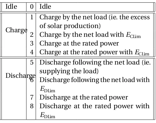
Table 2.1 Real-time Operation modes . . . 22
Table 2.2 Simplified modes of the ESD controller . . . 38
Table 2.3 Characteristics of the 190 houses selected . . . 39
Table 2.4 Time-of-use rate at HECO (located in Hawaii) . . . 40
Table 2.5 Simulation cases . . . 40
Table 2.6 Hawaii results for the 10 selected houses for a nine-month period, in $ 43 Table 3.1 Simplified modes of the ESD controller . . . 51
Table 3.2 List of the Different Algorithm Used . . . 55
Table 3.3 Statistical description of 149 houses selected . . . 61
Table 3.4 Time-of-use Rate in HECO (Hawaii Utility) . . . 61
Table 3.5 K Best Feature Selected . . . 62
Table 3.6 Statistical description of 50 houses selected . . . 66
Table 3.7 Time-of-use Rate in HECO (Hawaii Utility) . . . 68
Table 3.8 Savings results for the different cases using mode based control . . . . 71
Table 4.1 Simplified modes of the ESD controller . . . 78
Table 4.2 Statistical description of 149 houses selected . . . 87
LIST OF FIGURES
Figure 1.1 Resources Potential,[Tsa06] . . . 3
Figure 1.2 Emissions chart, source: union of concerned scientists . . . 4
Figure 1.3 PV Cumulative installation (source: DOE) . . . 5
Figure 1.4 California Duck Curve (source: CAISO) . . . 6
Figure 1.5 Global cumulative storage deployments, by country . . . 6
Figure 1.6 Global cumulative storage deployments, by application . . . 7
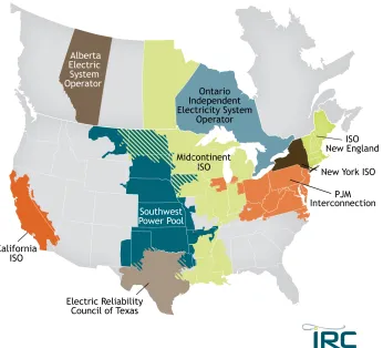
Figure 1.7 RTO, ISO map, source: FERC . . . 8
Figure 1.8 HECO ToU rate in 2015 . . . 10
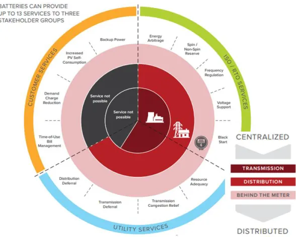
Figure 1.9 Batteries can provide up to 13 services, source: Rocky Mountain In-stitute . . . 12
Figure 1.10 Comparison of the energy storage value, source: Rocky Mountain Institute . . . 13
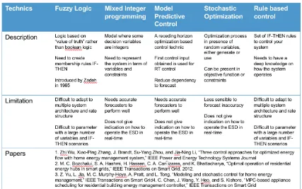
Figure 1.11 Comparison of existing methods for ESD control . . . 15
Figure 2.1 A description of the Narnet . . . 30
Figure 2.2 An illustration of the mode selecting process . . . 31
Figure 2.3 A description of the 24-hour Scheduling and real-time mode-based operation process . . . 32
Figure 2.4 Percentage of theoretical maximum achievable savings for 10 selected houses . . . 44
Figure 2.5 An example of the simulation results from one household . . . 44
Figure 2.6 Comparison of the PMSA savings for 190 houses in Austin, Texas: 7kWh/3kW versus 4kWh/2kW battery. . . 45
Figure 2.7 Impact of PV-to-load ratio on the PMSA savings for 190 houses in Austin, Texas. . . 46
Figure 2.8 Comparison of the PMSA savings for 190 houses in Austin, Texas: reduced mode versus full mode operation. . . 47
Figure 3.1 Mode-based control algorithms, on the left the EMPC approach, on the right the machine learning approach . . . 59
Figure 3.2 Performance using the K best features . . . 63
Figure 3.3 Accuracy of Each Machine Learning function of the Training Length with 7 features selected . . . 64
Figure 3.4 Precision of Each Mode Selection compared between the MPC Ap-proach and the NN with 20 neurons in one hidden layer . . . 65
Figure 3.7 Sensitivity analysis over the training length, in a case with 14 features,
and in different seasons . . . 67
Figure 3.8 Precision of Each Mode Selection compared between the MPC Ap-proach and the NN with 20 neurons in one hidden layer . . . 70
Figure 3.9 Boxplot representing the PMSA for the 4 months tested . . . 72
Figure 3.10 Scatter plot representing the PMSA depending on the ratio PV/load, for the EMPC with ALF, the NN 201 and RF 1000 . . . 73
Figure 3.11 Barchart representing the total cost of the 50 houses per season of test with three algorithms . . . 74
Figure 3.12 Barchart representing the mean PMSA of the 50 houses per season of test with three algorithms . . . 75
Figure 4.1 Proposed data structure for the shared learning . . . 82
Figure 4.2 Accuracy result for the first scenario . . . 89
Figure 4.3 Accuracy result for the second scenario . . . 90
CHAPTER
1
INTRODUCTION
Chapter 1 will present the context of the research, the contributions of this dissertation.
1.1
Context
Addressing climate change and decarbonizing our energy system is one of the main
chal-lenges that humanity is facing in the 21st century[UNE12; Mar07]. Paris accords[UNF15],
signed in December 2015, provide a global framework to stay on a pathway for the global
temperature to stay within the two degrees band. In order to achieve this goal, two changes
electrify-ing everythelectrify-ing.
Solar energy is one of the most abundant sources of energy on Earth[Tsa06], Fig. 1.1.
Indeed, the planet receives in one day enough energy to power human civilization for a year
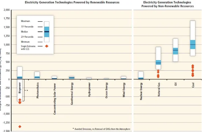
[Tsa06]. Solar is also the most abundant carbon-free emitting renewable resource, Fig. 1.2.
Industrial revolutions have been energy revolutions[SK12; FO14; Bar11], with first the rise of
coal and the steam engines that powered railway and allowed the first industrial revolution.
It was followed by oil and gas for the second industrial revolution. It is now headed toward
a third revolution that will be powered by carbon-free resources. Electricity will play an
increasing role. Electrifying everything[Bar; Ast17], electric vehicles replacing internal
combustion engine vehicles, electrification of heating and cooling systems, electrification
of cooking systems.
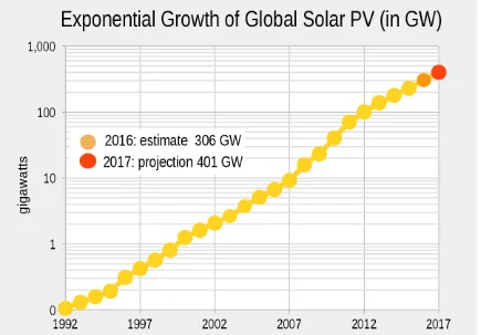
Solar Photovoltaic (PV) installations have been growing exponentially over the last
decade, Fig. 1.3. With the growth of human population in the 21st century combined with
the growth of energy needs, humanity will have to change its energy system to mitigate
climate change impact. PV is one of the electricity sources that emit the least CO2. However,
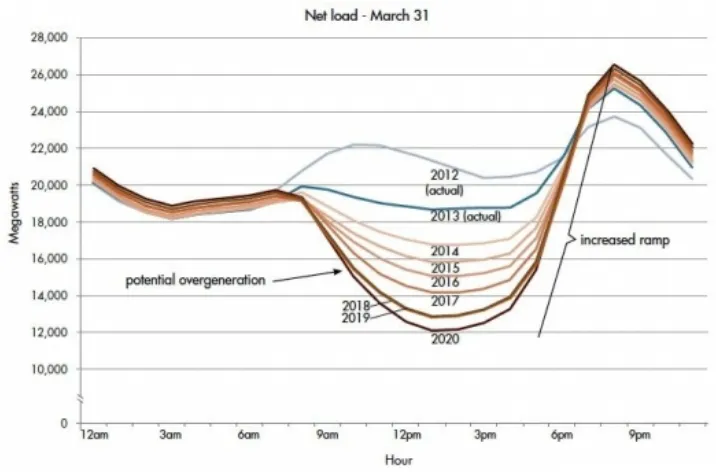
PV does not come without challenges. Intermittency and different seasonal outputs are at
the top of the list. One of its most famous illustrations is the CAISO "Duck Curve", Fig. 1.4,
from California that shows a lower and lower netload in the belly of the duck during the
day, and an increasing ramping need to match the demand of the evening peak, this ramp
is represented by the duck’s neck.
To mitigate those challenges, experts believe that energy storage can play a critical role.
Helping the system ride the short-term events (such as cloud passing, voltage flickering)
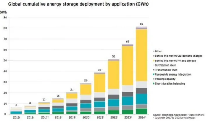
and reduce their impact on electricity grids. An exponential growth in ESS installations is
already underway, as shown in Fig. 1.5. Among the potential applications for energy storage,
Figure 1.2Emissions chart, source: union of concerned scientists
This deployment is being driven by a falling cost of lithium-ion batteries, while
elec-tricity prices are rising in almost every utility territory. Among the benefits for a customer
going solar+storage we can find: a lower electricity bill, backup power (if the inverter can
disconnect from the grid), cheap electricity to power an electric vehicle, a lower carbon
footprint in territories that rely on fossil fuel to produce electricity.
In the next section, the benefits of distributed energy storage will be discussed.
1.2
Why Distributed Energy Storage?
In the US, the electricity system is regulated by the Federal Energy Regulation Commission
(FERC) at the federal level. The North American Electric Reliability Corporation (NERC)
is responsible for developing and enforcing reliability standards for the electricity grid.
Figure 1.4California Duck Curve (source: CAISO)
Figure 1.6Global cumulative storage deployments, by application
components of the electricity grid are transmission, generation, and distribution. The
stakeholders of these different components are organized differently depending on whether
the market is competitive or an integrated monopoly. In a competitive market, the same
company does not own all the generation and distribution assets. An Independent System
Operator (ISO), or Regional Transmission Operator (RTO), as shown in Fig. 1.8, organize
the electricity markets. Integrated monopoly utilities own the distribution and generation
assets. Electric utilities can also be publicly owned and fall under the category of municipal
utility (owned by the city or town) or cooperative utility (owned by the customers it serves).
In 1996, there were more than 3,000 utilities in the US alone. Some of this utilities are
investor-owned, other are publicly owned. Some operate in cities, others in rural areas.
Some are in a territory with strong support for DERs. However, residential solar is getting
cheaper, soon enough it will be cheaper to obtain electricity through residential solar rather
than utilities. With massive adoption of distributed PV, voltage fluctuations, duck curves
Figure 1.7RTO, ISO map, source: FERC
be to acquire energy storage. With a large number of utilities, and with each one of them
having multiple tariffs for residential and light commercial customers, how can we design
a control algorithm for energy storage that can adapt to the different tariffs? Have strong
performance? And does not require heavy computation?
Furthermore, usual use cases for storage are frequency regulation, voltage support,
energy arbitrage for front-of-the-meter installations. For behind-the-meter applications,
we can find demand-charge management, peak shaving, ToU arbitrage, self-consumption.
To address this diversity of rates and behind-the-meter applications, an algorithm to
minimal modifications.
1.2.1
Retail Electricity Structure
Over the years, retail electricity rates have evolved in different forms depending on
legisla-tures, PUC rulings and generation mix. Among the most frequent rate structures we can
find:
• Flat Rate: a fixed price in $/kWh, does not change with time of volume consumed;
• Time-of-Use (ToU): different prices for different periods of the day, usually referred
to a peak price (highest price of the day), off-peak price (lowest price of the day),
shoulder price (between the peak and off-peak prices);
• Demand Charge: the highest peak of the month is billed $/kW;
• Tiered Rate Plan: the price of electricity evolve with the total consumption during a
billing cycle, for example, there is a price for all energy consumed below 1 MWh, a
higher price for the consumption above 1 MWh;
• Critical Peak Pricing (CPP): an event that can be triggered by a utility
• Dynamic Pricing: send in advance to the customers a steep increase in the electricity
prices with the goal to reduce peak demand;
• Real-Time Pricing: the customer would pay an ever-changing price based on the
current market prices
Those are the current rate structure. In the literature and business circles, other
mecha-nisms or organization of markets are being discussed. Among the ones getting the most
traction, we can find virtual power plants (VPP), microgrids, aggregators, DSO (independent
distributed system operators) and transactive energy.
Figure 1.8HECO ToU rate in 2015
grid;
• VPP: is a cloud-based distributed power plant that combines the capacity of DERs for
the purposes of as well as trading on the electricity market.
• Microgrid: is local grid comprised of generation, distribution assets and loads. Can
be disconnected from the main grid;
• DSO: independent distribution system operator with the goal to operate a market
on the distribution side to enhance renewable integration into the grid and take
• Transactive Energy: â ˘AIJa system of economic and control mechanisms that allows
the dynamic balance of supply and demand across the entire electrical infrastructure
using value as a key operational parameter.â ˘A˙I per NIST definition.
1.2.2
Benefits of DER to the Grid
DER benefits to the grid is not a new topic of interest for researchers,[Ian03; Bai03]. Studies
already found certain advantages using distributed resources to increase the reliability of
grids and reduce the cost of electricity.
More recent studies[Sha17; Fit15]found that energy storage could provide up to 13
services to the grid. From Fig. 1.9 we can observe that only behind the meter storage can
provide all the mentioned services. The proposed services range from frequency regulation
to black start through PV self-consumption and ToU arbitrage. While DER provide benefits
to the grid through this wide range of services, not all of them provide the same economic
value. In Fig. 1.10 from[Fit15]we can see a comparison of the monetary benefits of different
storage service across different studies. It can be observed that the most value is found
in T&D deferral, where energy storage can delay the investment in a new substation or
transmission line. For behind-the-meter applications, it can be observed that every service
bring value to the customer. Today, the value for self-consumption is low, however, it is
getting higher and higher in areas with high electricity prices with low PV export valorization
such as Hawaii, Germany, and Australia.
1.3
Challenges and Contribution
This dissertation focuses on methods to control energy storage devices. The methods
Figure 1.9Batteries can provide up to 13 services, source: Rocky Mountain Institute
control, and heuristic. In the optimization based approaches, we can find mixed-integer
optimization (MIP), model predictive control (MPC) or multi-stage optimization. In the
heuristic category, we can find the rule-based control algorithms or fuzzy logic.
Optimization in HEMS has been using multiple approaches in order to achieve multiple
objectives as minimizing the impact on the comfort or minimizing the cost[Yu13; DL11;
Cha13; MR10]. Optimization has been used to operate energy storage for different
appli-cations as DER integration, microgrid operations or being used coordinately with HEMS.
Different approaches have been developed as Mixed Integer Programming (MIP),
Con-tinuous Relaxation (CR) or stochastic optimization[Wang2016ASystems; Che11; Boz12; Wan14; HG12; Guo12; Zhi15; Tan13].
Model Predictive Control (MPC) is a powerful receding optimization based control
scheme. It has been used for HEMS to control TCL and non-TCL loads[Che13]and[NL14].
Figure 1.10Comparison of the energy storage value, source: Rocky Mountain Institute
storage in large power systems applications as well as for hierarchal control for residential
applications[LampropoulosHierarchicalGeneration; Bak16; Li15; Gar12].
[Raw12]presents the principles of Economic Model Predictive Control (EMPC). MPC
will optimize based on a setpoint, coming from an ad-hoc steady-state analysis. EMPC
minimizes directly the cost in the objective function. EMPC has been used as well for power
management either for controlling a fleet of refrigerators for demand-response purposes or
for climate control in commercial buildings[Hov10; Jin11; Hov11; Ma15]. In this paper, we
propose an EMPC-based algorithm to schedule energy storage for residential applications.
Fuzzy logic and multi-scale optimization can be the comparable approach for real-time
control. The first one presets control strategies based on price and SOC conditions. The
second one is optimizing the system as close as real-time as possible. Fuzzy logic would be
the closest to the proposed solution in this paper, as based on SOC and electricity prices
prediction is taken into account as well, the problem becomes more complex and is not
easily adaptable to multiple locations and pricing scheme. The Fuzzy approach is not based
on optimization; therefore, the optimum cannot be guaranteed.
Regarding the multi-scale optimization as in[LampropoulosHierarchicalGeneration] or in[YM14], the real-time control will minimize the deviation between the mismatch of
the forecast and the objective established during the day ahead or hour ahead optimization.
However, these objectives are highly dependent on the forecasted value and are subject to
significant errors. Moreover, it does not indicate how to reach the SOC objective: by charging
or discharging at full power or following the solar or load profile. Another drawback of the
multi-scale optimization is that the real-time control follows one objective, as minimizing
the backfeed. However, depending on the conditions, another real-time control operation
objective is necessary to reach the optimal control. For example, in a net-metering case,
maximizing the back-feed during peak hours is more economical.
Heuristic approaches, especially the rule-based control algorithms, can yield high
per-formance for simple ToU rates, or other simpler tariff structures. The computation power
required is also low. However, these methods would require a certain number of
human-hours in order to tune and develop an RBC algorithm for each application and maintain the
algorithms after each change of tariff. In the US alone, we can find more than 3000 utilities
and each utility has multiple rates for each class of customer, which might not be practical.
On the other hand, the optimization-based approach does not require a large number of
human-hours to tune the algorithms to each tariff. The main drawback for an optimization
based algorithm is the requirement to solve the optimization problem in almost real-time,
which is a pre-requisite in order to adapt to forecast inaccuracies.
In order to address this two challenges, and combine the generalization of an
Figure 1.11Comparison of existing methods for ESD control
forecast inaccuracies, we introduce a mode-based control approach. Using an
optimization-based discrete mode approach allows reducing the frequency of solving an optimization
problem from one per minute to one per hour. In order to further reduce the real-time
computation need, we propose to train a machine learning to learn what mode to select
depending on operational conditions. To reduce the need for temporal data, requiring a
few months of historical data, before being able to train an ML algorithm, we introduce the
shared learning approach.
Machine learning for HEMS has been proposed before[Rue16; Zha16; Wei15; Wan15],
they can fall into two categories. The first, for model-free application, the RL algorithm can
derive a model. The second one, to tune a parameter in an optimization objective. This
address the control decision issues while the second one relies on an optimization problem
to find the optimal control decisions. A supervised learning approach is proposed. The
advantage of this approach is to use the historical data to 1) make the control decision 2)
bypass the optimization and reduce the real-time computation needs.
In Chapter II, the mode-based approach is introduced. The main contributions are
the introduction of the modes, an algorithm to select the mode for the next time step
followed by simulation results to demonstrate the performance of this approach. It can
be observed that using a mode-based algorithm yields the same results as a continuous
optimization-based controller with a perfect forecast. Performances are increased with a
non-perfect forecast. The usage of an average load forecaster (average load of the year as a
constant forecast) yields better performance than using a neural-network-based forecaster.
Chapter III introduces a machine learning (ML) approach to select the modes and
increase the performance of the controller. Once enough historical data is generated, an
ML model is trained on the data. This approach, with sufficient data (approximately nine
months to reach plateau accuracy), outperforms the mode based algorithm with EMPC.
This approach allows to have fast and easy computation on distributed hardware (for
example a neural network with 20 neurons in one layer is used) and to send the bulk of the
computation to the cloud to train the models. Another advantage of this method is to not
rely on a load forecaster to select the next mode.
A drawback of this approach is the necessity for nine or more months of data for each
house. Chapter IV presents a multi-agent shared learning algorithm. The goal is to share
the same training set across all the controller agents. One agent is the learning aggregator
that will centralize the training sets and historical data and will be in charge of training the
model and keeping it updated. It will then send the trained model to each battery agent.
accuracy with as little as two months of data. It is also shown that a high accuracy can be
reached with distinct houses in the training and testing sets.
1.4
Organization of the Dissertation
The rest of the dissertation is organized as follows. Chapter II introduces the design of
the real-time operation modes and the architecture of the mode-based control approach.
Chapter III presents the Machine Learning method to control an ESD. Chapter IV introduces
the multi-agent approach to the learning problem. The conclusions and future work are
CHAPTER
2
A MODE-BASED ENERGY STORAGE
CONTROL APPROACH
2.1
Introduction
High penetration of residential and commercial rooftop photovoltaic (PV) systems may
increase power fluctuations in distribution feeders and reverse power flow directions. As a
result, utilities may experience voltage issues, such as over-voltage, large voltage ramps, and
voltage swings. The intermittency of the solar generation resources and backfeeding power
while in Hawaii, backfeeding is no longer allowed for newly installed PV systems[201].
Therefore, installing energy storage devices (ESDs) to store excess solar power and smooth
power fluctuations is an increasingly attractive option for residential and commercial PV
systems. Another key driver for residential and commercial ESD adoption is the increase in
reliability and resiliency to have backup power supplies during blackouts[Ard17].
The main ESDs used for residential PV applications are different types of battery storage
systems. In[DiO15]lithium-ion and lead-acid are compared for small residential projects.
Findings show that lithium-ion batteries can yield positive net present values while
lead-acid cannot due to high recurring capital cost. Profitability remains highly dependent on
the battery economics. The objectives of scheduling and dispatching the battery systems
include minimizing utility bills[HG12; VDV13], smoothing PV outputs, maximizing
self-consumed solar energy[Wan15], and providing different grid services[GP13; Got16]. A
variety of optimization methods, such as Dynamic Programming[Liu14], Fuzzy Logic
[Zhi15], Mixed Integer Programming (MIP)[Boz12], and Stochastic Programming[Yu13]
have been proposed to solve these scheduling issues and dispatch the battery power outputs
in real-time. Among them, the most commonly used approach is the MIP-based approach
that can find the optimal power outputs of the battery at each dispatch interval over a given
scheduling period considering its operational constraints.
However, the MIP-based methods are sensitive to the accuracy of the load, PV, and
price forecast. Unfortunately, for realistic residential load and PV data sets, day-ahead load
forecast error is approximately 20%[Ste17; Gen15]. The forecast accuracy of PV power
outputs depends on the type of day. On a cloudy day, the forecast error can be over 50%
[Lon12; Nii12]. In this error range, the optimality of the schedule obtained by the MIP
methods will no longer hold. To cope with the forecasting errors, multi-stage algorithms (e.g.
based on 24-hour load and PV forecasts. Then, the schedule is adjusted every hour or every
few minutes based on the updated forecast values.
All algorithms described previously determine the optimal battery power outputs to
meet a specific objective, such as minimizing payment or smoothing the power
fluctua-tions. In practice, customer electricity consumption patterns may change and utility rate
structures may vary. As a result, the battery operation varies significantly from customer to
customer, making it challenging for manufacturers to design a universal battery controller
that achieves a longer lifetime and higher efficiency.
Oftentimes, for residential applications, the main issue for controlling batteries is
de-ciding how to charge and discharge instead of determining the optimal charging and
discharging power. Assume that a battery storage system can be equipped with a controller
with a set of built-in, real-time control modes. In this paper, we present a novel mode-based
control approach so an external controller will control the operation of a battery system via
selecting one of its built-in control modes. The design of the real-time control modes is first
introduced; then, a two-stage algorithm for real-time optimal mode selection is presented.
In the first stage, a 24-hour economic model predictive control (EMPC) algorithm is used
to determine the optimal battery power outputs for the next 24 hours. Then, based on
the optimal power output of the next hour, unsuitable modes for the next operating hour
are eliminated. In the second stage, assuming that the battery is operating at one of the
suitable modes in the next hour, run the 24-hour EMPC again to calculate the total cost.
Select the mode with the lowest cost to be the operation mode for the next hour. Note that
a distinct difference between our approach and the approaches described previously is
that, instead of calculating the optimal hourly battery charging and discharging power, the
optimal battery operation mode is selected for the next hour.
in the PECAN street project[Pec]. The simulation results demonstrate that the mode-based
approach outperforms the MIP-based approach consistently and shows less sensitivity to
PV and load forecasting errors and load pattern changes.
The main contributions of the paper are twofold. First, we designed nine primary
real-time operation modes for charging and discharging residential energy storage systems
that cover a wide range of battery operation conditions. Second, we developed a two-stage
mode selection algorithm to select the operation mode for real-time operation. To the best
of the authors’ knowledge, such algorithm has never been proposed for residential energy
storage applications.
The rest of the paper is organized as follows: Section II introduces the design of the
real-time operation modes and architecture of the mode-based control approach. Section
III presents the problem formulation. The simulation setups and results are discussed in
Section IV. The conclusions and future work are summarized in Section
2.2
Real-time Operation Modes
The main advantage of using a mode-based control approach is to allow the battery
manu-facturers to provide a set of standardized operation modes in the battery controller that can
be fine-tuned to achieve desired performances (e.g. high efficiency and long lifetime) at the
battery cell level. Because the external controller only needs to select the best mode from
a few build-in modes for the battery system to work at, the control and sensing tasks can
be distributed to the battery controller and make the battery system a truly plug-and-play
device. Fundamentally, this approach belongs to distributed, discrete control because it
focuses on finding the best combination of a set of modes to realize a variety of control
the complexity of both the battery controller and the external controller will also increase.
Therefore, in this paper, we introduce 9 real-time operations modes: 4 charging modes, 4
discharging modes, and 1 idling mode, as shown in Table 2.1. In this paper, the application
Table 2.1Real-time Operation modes Idle 0 Idle
Charge
1 Charge by the net load (ie. the excess of solar production)
2 Charge by the net load withECLim 3 Charge at the rated power
4 Charge at the rated power withECLim
Discharge
5 Discharge following the net load (ie. supplying the load)
6 Discharge following the net load with
EDLim
7 Discharge at the rated power
8 Discharge at the rated power with
EDLim
we select for illustrate how the mode-based approach works is:minimizing the customers
utility bill under the time-of-use rate. This application is selected because it is the most
commonly used application in practice. In addition, because actual load data and utility
rates can be used in case studies, meaningful performance comparisons can be made
with existing methods (e.g. MIP-based algorithms) to benchmark the performance of the
mode-based algorithm.
2.2.1
Control Logic of the Idling and Charging Modes
Because the main goal of charging batteries in residential PV applications is storing excess
to meet those control objectives. First, let the battery power output,PB, be positive when
charging and let the net load,Pnet, be positive if the load exceeds the solar generation. Second, let the mode selection happen at the beginning of each hour and let the minimum
operation period for each mode be an hour. During theithhour, the mode controller will adjust battery power,PB(j), every minute. Thus,∆t =1/60 hour, j =1...60, andi =1...24.
DefinePCLim(j)as the charging limit set by the customer for thejthinterval andECLimas the energy charging limit for the hour.
Based on those assumptions, at the jthtime interval, the netload,P
net(j), is calculated as
Pnet(j)=Pload(j)−Psol(j) (2.1) Based on the battery energy level, EB(j), and the battery energy limit,Emax, the battery charging power cap,PCCap(j), is calculated as
PCCap(j)=
Emax−EB(j)
/∆t (2.2)
Then, the battery charging power of modem at the jthtime interval,P
as
PB(j)|1=max
0, minPCCap(j),PCLim(j),−Pnet(j),Prated
(2.3)
PB(j)|2=
PB(j)|1, if
j
P
j=1
PB(j)|1∆t
<ECLim
0, otherwise
(2.4)
PB(j)|3=max
0, minPrated,PCLim(j),PCCap(j)
(2.5)
PB(j)|4=
PB(j)|3, if
j
P
j=1
PB(j)|3∆t
<ECLim
0, otherwise
(2.6)
In the "idling" mode, the battery output is simple zero, so we have,
PB(j)|0=0 (2.7)
2.2.2
Control Logic of the Four Discharging Modes
Because the main goal of discharging ESDs in residential PV applications is supplying load
at high price periods or using self-generated power, we designed four discharging modes
to meet those control objectives. Similar to the charging modes, at thejthinterval of theith hour, we fist calculate the battery discharging power capPDCap(j), as
PDCap(j)=
EB(j)−Emin
/∆t (2.8)
DefinePDLim(j)as the discharging limit set by the customer andEDl i mas the discharge
ithtime interval,P
B(j)|m, is calculated as
PB(j)|5=−max
0, minPDCap(j),Pnet(j),PDLim(j),Prated
(2.9)
PB(j)|6=
PB(j)|5,
j
P
j=1
−PB(j)|5∆t
<EDLim
0, otherwise
(2.10)
PB(j)|7=−max
0, minPrated,PDLim(j),PDCap(j)
(2.11)
PB(j)|8=
PB(j)|7,
j
P
j=1
−PB(j)|7∆t
<EDlim
0, otherwise
(2.12)
Based on (4.5)-(2.12), battery manufacturers can implement the build-in modes at the
battery controller level. An external controller, such as a home energy management system
controller, can simply control the battery system by letting it operate at one of the 9 modes
instead of trying to determine the actual battery power outputs for the battery system at each
time interval. This can greatly simplify the interface between the external controller and the
battery systems, making the battery system plug-and-play with guaranteed performance.
In the next section, we are going to introduce the method for selecting the best operation
mode.
2.3
Mode-based Controller Design
In this section, we will introduce the economic model predictive control (EMPC) algorithm,
2.3.1
Economic Model-predictive control (EMPC) method
In[Che13] [Gar12], the authors introduced the model-predictive control (MPC) method
to minimize the deviations from given setpoints. In[Raw12], the authors proposed the
EMPC method to determine the setpoints for the ESD controller instead of minimizing
the deviations from the setpoints sent to the ESD controller using the 24-hour price, load,
and PV forecast as inputs. In this paper, we adapted the EMPC approach to determine the
optimal hourly setpoint for the battery power over the next 24-hour period. The objective
function of the EMPC problem is to minimize the 24-hour cost considering the cost of
import and export energy as well as the cost for battery degradation, so we have
z(u1(i))=min 24 X
i=1
Cexport(i)Pexport(i)∆T(1−u1(i))+
Cimport(i)Pimport(i)∆T u1(i) +Ncycle(i)Ccycle(i)
s.t.
Pimport(i)−Pexport(i)−Pcharge(t) +Pdischarge(t)
=Pload(i)−Psol(i) (2.14)
Emin≤EB(i)≤Emax≤Erated (2.15) 0≤Pcharge(i)≤Pchargemax (2.16) 0≤Pdischarge(i)≤Pdischargemax (2.17) 0≤Pimport(i)≤Pimportmax (2.18) 0≤Pexport(i)≤Pexportmax (2.19)
Pimport,Pexport,Ncycles,Pcharge,Pdischarge≥0
where
u1(i) =
1 if Pimport(i)>0 0 if Pexport(i)>0
(2.20)
u2(i) =
1 if PB(i)≥0
0 if PB(i)<0
(2.21)
Pimport(i) =max
0,Pload(i)−Psol(i)−PB(i)
(2.22)
Pexport(i) =max
0,Psol(i)−Pload(i)−PB(i)
(2.23)
EB(i) =EB(i−1) +u2(i)ηPcharge(i)∆T− (1−u2(i))
Pdischarge(i)∆T
η (2.24)
Echarge= 24 X
i=1
Pcharge(i)∆T (2.25)
Edischarge= 24 X
i=1
Pdischarge(i)∆T (2.26)
Ncycles=
Echarge+Edischarge 2Er a t e d
(2.27)
Pcharge(i) =PB(i) (2.28)
Pdischarge(i) =−PB(i) (2.29)
Note that because the EMPC calculates hourly schedules,∆T =1 and can be omitted
from the problem formulation. We also used a simplified method to calculate the number
of battery cycles in (2.40). More sophisticated methods for estimating the effective battery
cycles to account for degradation can be used, but because our focus is to formulate the
mode-based control algorithm we chose to use a simplified battery cycle calculation as an
2.3.2
Forecast Methods
One of the main motivation for the development of the mode-based approach is to make
the ESD dispatch less sensitive to the accuracy of forecast methods. Therefore, it is critical
that the performance of the proposed algorithm is tested when using different forecasting
methods and compared with the MIP-based approach. The EMPC algorithm requires price,
load, and PV forecast as inputs. Because we use the time-of-use rate as an illustration of the
mode-based control approach, price forecast is no longer required. So we consider mainly
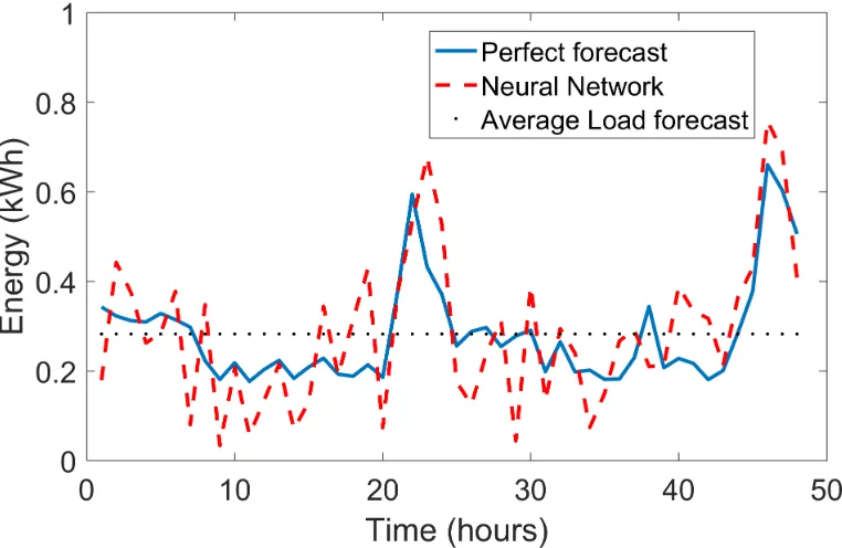
the accuracy of the load and PV forecast in our case studies. In[Hen17], we described 3
forecasters (see Fig. 2.2, a perfect forecaster, a average load forecaster and a neural-network
based forecaster. We have demonstrated that for the mode-based controller, an average load
forecaster outperforms a neural-network forecaster. Note that the average load forecaster
is the the yearly average load used as a constant forecaster. The mode-based controller
schedules the battery power in real-time for intra-hour operation; therefore, no PV forecast
is needed.
It is well known that the residential end use is highly random and its variations are
highly volatile, making accurate load forecast hard to achieve. To compare the robustness
of the algorithm with respect to the accuracy of the load forecast, we set up three cases. In
case 1, the actual load profile is used so forecast error is zero; in case 2, a neural network
forecaster is used; in case 3, a daily average load is used. The neural network forecasting
algorithm we selected is introduced in[Yan13]. The Narnet is a nonlinear autoregressive
neural network and has 25 neurons in the first layer and 10 in the second, as shown in Fig
2.1.
The Matlab Neural Network toolbox is used to create, train, and use the neural network.
Figure 2.1A description of the Narnet
and historical load data. The forecaster has a 5% forecast error on the OpenEI[Ope]data
and 50% error on the Pecan Street data[Pec]. To obtain this comparison, we trained each
forecaster with 6 months of data. For this paper, the forecaster is initially trained with 3
months of historical data. Then, at the beginning of each month, the data from all previous
months are used to retrain the model. In the third case, we used a load forecaster that
forecasts the average load for the whole day such that an expected load to solar output ratio
is obtained to determine whether the energy storage should charge or discharge. Figure 2.2
shows an example of the outputs of the three load forecast methods. The blue line is the
actual load profile used to obtain the optimal charging and discharging schedule. The red
dotted line is the output from the neural network forecaster. As can be seen in the figure,
the forecasting error is large when forecasting individual household loads, although the
general trend of the actual curve can be captured. The black dotted line represents the
average daily load forecast. Note that the average load forecast can be forecast relatively
accurately from the historical data because the daily electricity consumption is relatively
Figure 2.2An illustration of the mode selecting process
2.3.3
Mode Selection
In the mode-based approach, the external controller no longer sends setpoints (i.e.PB(i)
orPB(j)) to the battery system for controlling its real-time operation. Instead, the controller
lets the battery system operate in one of the 9 modes listed in Table 2.1. To select the best
mode, a straightforward approach is in reference toP∗B(i), the optimal hourly battery power
calculated by EMPC. Therefore, in the first stage, based on the 24-hour ahead forecast of PV,
load, and price, 24-hour ahead optimal hourly battery power outputs,P∗B(i), are obtained
using (2.33) for optimizing the energy bill for the next 24-hour period (e.g.i =1...24), as
shown in Fig. 2.3.
Based on the optimal action the battery should take for the next hour (i.e.P∗B(1)), one
EMPC 24-hour Ahead Scheduling Window
Determine
𝑃𝑃
𝐵𝐵
∗
𝑖𝑖
,
𝑖𝑖
= 1 … 24
,
𝐸𝐸
𝐶𝐶𝐿𝐿𝐿𝐿𝐿𝐿
,
𝐸𝐸
𝐷𝐷𝐿𝐿𝐿𝐿𝐿𝐿
,
𝑓𝑓
,
𝐶𝐶
𝑡𝑡𝑡𝑡𝑡𝑡𝑡𝑡𝑡𝑡
∗
𝑗𝑗
60
1
2
…
𝟏𝟏
𝟐𝟐
…
𝒊𝒊
𝟐𝟐𝟐𝟐
Hourly Mode-based Operation Window
Determine
𝑚𝑚
∗,
𝑃𝑃
𝐵𝐵
(
𝑗𝑗
)
,
𝑆𝑆𝑆𝑆𝐶𝐶
(
𝑗𝑗
)
,
𝑗𝑗
= 1 … 60
,
𝐶𝐶
1
.
…
…
Figure 2.3A description of the 24-hour Scheduling and real-time mode-based operation process
should charge at 2 kW for the next hour (i.e.P∗B(1) =2k W), all the discharging modes are
eliminated and all the charging modes are selected for the next stage comparison. Note
that although an EMPC based approach is used in this case to minimize the bill for the user
over the 24-hour period, one can use other methods for obtaining the operational trends.
At the end of each first stage, we obtain the total cost of the 24-hour scheduling period,
C∗
total|i=1...24=z1, the optimal ESD output for the next operation hour,P ∗
B(1), and all feasible
battery operation modesf. In addition, to determine the charging and discharging energy
limit for modes 2, 4, 6, and 8, we have
ECLim=P ∗
B(1)×∆T i f P
∗
B(1)>0 (2.30)
EDLim=−P ∗
B(1)×∆T i f P
∗
B(1)<0 (2.31)
In the second stage, for each feasible mode, we calculate the minute-by-minutePB(j)|f
calculated based onPB(j)|f. UsingS O C(60)|f as the initial condition, we run EMPC again
for periodi=2...24 to calculatez2|f. Then, the total cost is calculated by
Ctotal∗ |f =C(1)|f +
24 X
i=2
C∗(i)|f =C(1)|f +z2|f (2.32)
After we obtain the total cost for the next day for each feasible mode, the mode with the
least cost can be selected. If the total cost of the optimal mode exceedsk% of the optimal
Algorithm 1Mode-based Control Algorithm
1: Calculatez1,P
∗
B(i), andu∗2(i)for the scheduling periodi=1...24 use (2.33).
2: Useu∗
2(1)andP
∗
B(1)to determine the feasible modes.
3: if u∗
2(1) =1then
4: Eliminate discharging modes sof ∈[0, 1, 2, 3, 4]
5: EClim=P
∗
B(1)
6: elseu∗
2(1) =0
7: Eliminate charging modes sof ∈[0, 5, 6, 7, 8]
8: EDlim=−P
∗
B(1)
9: end if
10: forRun feasible modes without hourly energy limit (i.e. if charging, run Modes 1 and 3; if discharging, run Modes 5 and 7)
11: iff =1 (same process for Modes 3, 5, and 7)then
12: CalculatePB(j)|1,S O C(j)|1, andC(1)|1
13: Calculatez2|1fori=2...24 using (2.33)
14: Ctotal|1=C(1)|1+z2|1
15: end if
16: end for
17: Select mode with the least cost,f∗=m i n(C
t o t a l|f)
18: ifCtotal|f∗>k×z1then
19: Enforce hourly energy limit, i.e.f∗=f∗+1
Algorithm 2Mode-based Control Algorithm
1: Select the optimal charging modem∗as follows:
Ct o t a l|1<Ct o t a l|3<k×z1 S e l e c t m o d e 1
Ct o t a l|3<Ct o t a l|1<k×z1 S e l e c t m o d e 3
Ct o t a l|1<k×z1<Ct o t a l|3 S e l e c t m o d e 1
Ct o t a l|3<k×z1<Ct o t a l|1 S e l e c t m o d e 3
k×z1<Ct o t a l|1<Ct o t a l|3 S e l e c t m o d e 2
k×z1<Ct o t a l|3<Ct o t a l|1 S e l e c t m o d e 4
2: Select the optimal discharging modem∗as follows:
Ct o t a l|5<Ct o t a l|7<k×z1 S e l e c t m o d e 5
Ct o t a l|7<Ct o t a l|5<k×z1 S e l e c t m o d e 7
Ct o t a l|5<k×z1<Ct o t a l|7 S e l e c t m o d e 5
Ct o t a l|7<k×z1<Ct o t a l|5 S e l e c t m o d e 7
k×z1<Ct o t a l|5<Ct o t a l|7 S e l e c t m o d e 6
k×z1<Ct o t a l|7<Ct o t a l|5 S e l e c t m o d e 8
2.3.4
Reduced Mode Operation
To simplify the operation, one can use a subset of the 9 modes defined in Table 2.1. In
the next section, we will model reduced modes operation, in which case, the five modes
described in Table 2.2 will be used. By comparing the performance with the full-modes
cases, one can determine what the marginal benefits are to have any additional mode. The
The reduced mode operation optimization problem can be formulated as follow:
z(i)=min 24 X
i=1
Bexport(i)Pexport(i)∆T+
Bimport(i)Pimport(i)∆T +Ncycles(i)Bcycle
(2.33)
s.t.
Pimport(i)−Pexport(i)−Pcharge(t) +Pdischarge(t)
=Pload(i)−Psol(i) (2.34)
Emin≤EB(i)≤Emax≤Erated (2.35)
0≤Pcharge(i)≤Pchargemax (2.36)
0≤Pdischarge(i)≤Pdischargemax (2.37)
0≤Pimport(i)≤Pimportmax (2.38)
Ncycles(i)=
|EB(i)−EB(i−1)| 2Er a t e d
(2.40)
EB(i) =EB(i−1) +ηPcharge(i)∆T−
Pdischarge(i)∆T
η (2.41)
Pimport,Pexport,Ncycles,Pcharge,Pdischarge≥0
i ∈[1, ..., 24]
Algorithm 3Control Algorithm for Reduced-mode Operation
1: Steps 1-17 are the same as the full mode operation
2: Select the optimal charging modem∗as follows:
...
k×z1<Ct o t a l|1<Ct o t a l|3 S e l e c t m o d e 1
k×z1<Ct o t a l|3<Ct o t a l|1 S e l e c t m o d e 3
3: Select the optimal discharging modem∗as follows:
...
k×z1<Ct o t a l|5<Ct o t a l|7 S e l e c t m o d e 5
Table 2.2Simplified modes of the ESD controller Idle 0 Idle
Charge 1 Charge by the net load,|Pnet|, ifPnet< 0
3 Charge by the rated power,Prated Discharge5 Discharge following the net load,
|Pnet|, ifPnet>0
7 Discharge by the rated power,Prated
2.4
Simulation Results
The simulation setup, performance evaluation criterion, and simulation results are
pre-sented in this section.
2.4.1
Simulation Setup
Data collected in the Pecan Street project[Pec]are used to benchmark and validate the
performance of the proposed mode-based approach. We select 190 houses in Austin, Texas
for the study. All households have sub-metered data for PV and total load with
minute-by-minute data points in year 2015 (i.e. 365×24×60 data points). So, each simulation run is 1 year with 1 minute interval. The characteristics of this data set is summarized in Table 4.2.
We used the residential household electricity consumption data set collected by the
Pecan Street project[Pec], which can be downloaded at http://www.pecanstreet.org. Both
customer electricity consumption and roof-top PV outputs are available in the Pecan Street
data set. As shown in Table??, 10 houses across three states were selected. Their yearly energy consumption vary between 2.3 and 21.77 MWh to simulate small, medium and
large residential loads. Among the ten households, eight are equipped with roof-top PV
for zero-energy, undersized, oversized).
Another set of data from Pecan Street has been used. We selected all the houses from
Austin, with PV that have 8760 points over the year 2015, the characteristics of this data set
is shown in Table 4.2. The total number of houses matching these criteria is 190 houses.
Table 2.3Characteristics of the 190 houses selected
Base Case ($) Load (kWh) Solar Gener-ation (kWh) Ratio PV/load
Mean 1,763 12,070 7,022 0.66
Standard
deviation 1,006 5,657 2,590 0.27 Maximum 10,086 51,466 20,416 1.57
Minimum 500 3,533 528 0.05
1st
Quar-tile 1,158 8,606 5,448 0.45
3rd
Quar-tile 2,154 14,340 7,907 0.83
Median 1,552 10,803 6,946 0.64
Hawaii time-of-use (TOU) rate (See Table 4.3) is used in the simulation so no price
forecast is not needed. In Hawaii, no backfeed is allowed so the main goal for controlling
energy storage systems is self-consuming solar generation and shifting consumption to
low price periods. Six scenarios (See Table 2.5) are simulated to compare the performance
of the mode-based algorithm with the base case and the MIP-based EMPC algorithm
when using different forecaster. Case 1 is designed to demonstrate the optimality of the
mode-based approach so we assume in this case the load forecast is perfect. Case 2 is
Table 2.4Time-of-use rate at HECO (located in Hawaii)
Price (c$) Hour weekday Hour weekend Off peak 18.21 9 PM -7 AM 9 PM - 5 AM Shoulder 23.71 7 AM - 5 PM 5 PM - 9 PM
Peak 26.71 5 PM - 9 PM
-accuracy. An average load forecast is a very inaccurate energy forecaster comparing with
other sophisticate forecasters as it only gives a daily average load. We will demonstrate how
optimality will be influenced if such a forecaster is used. Then, we demonstrate reduced
mode operation, in which case 5 modes (see Table 2.2) instead of 9 modes (see Table 2.1) are
used. This case compares whether or not additional modes are needed. To compared the
Table 2.5Simulation cases
Case Description
Base Case Base case with no battery installed EMPC MIP-only optimization with a Perfect forecaster Case 1 Perfect forecast+mode-based control
Case 2 Constant average load forecast+mode-based control Case 3 Simplified modes and perfect forecast
Case 4 Simplified modes and average load forecast
influence of the battery size, we modeled two battery sizes: 7kWh/3kW and 4kWh/2kW. In
both case, the charging and discharging powers are the same and the round trip efficiency
2.4.2
Performance Evaluation Criterion
To evaluate the performance of different cases, we calculate the percentage of the maximum
savings achieved,P M S A, for each house in the data set as
P M S A= Cbase−Ccase Cbase−CEMPC
(2.42)
whereCbaseis the annual cost of the base case where no battery is installed;CEMPCis the annual cost of the EMPC plus perfect load forecast case so it represents the optimal cost;
Ccaseis the cost of the four mode-based control cases described in Table 2.5. The annual cost is calculated as
C =
365×24 X
i=1 X60
j=1
Pimport(i,j)×Cimport(i,j)
(2.43)
wherePimport(i,j)can be calculated using (2.34) andCimport(i,j)is the TOU rate. Note that because we used the Hawaii TOU rate, backfeeding power is not allowed so it is not paid.
Therefore, in (2.43), there is no export related revenue.
2.4.3
Results for Multiple-Houses
In Fig. 2.5, the load is shown by the blue surface and the solar by the yellow surface. The
black continuous line is the discharge based on the mode selection and the red dotted line
is the discharge based on the MIP-only results. The blue line is the electricity price at a given
moment. With this figure, we can observe that if we follow the MIP-only control actions,
the battery will sometimes over-discharge or under-discharge due to the inaccuracy of the
the discharge has a closer match to the shape of the load.
We presented the simulation results in Fig. 2.4 and Table 2.6 for 10 households using
the Hawaiian rate. In Table 2.6, we show the total cost for each case and each house over
a nine-month period using the Hawaiian tariff. In Fig. 2.4, we plotted the distribution
of the percentage of potential savings achieved for each house. The maximum potential
savings are calculated with the difference between the base case, Case 1, and the MIP-only
scenario and perfect forecast, Case 2. For each case, we calculate the percentage of this
value achieved.
From Fig. 2.4, it can be observed that the mode scheduling based algorithm always
achieved close to 100% of the potential saving calculated in the case 5, optimization+
perfect forecast. We can also observe that the case combining mode scheduling and average
load forecast gets results comprised between 75% and 95%. Houses 9836, and 624, that
have the most PV got results>90%. It can also be observed that on average the
mode-based scheduling performance are greater than in the case of EMPC only. We can deduce
that the mode-based control is less sensible to the forecast accuracy. The impact of the
forecaster on the results can be observed as well. For EMPC algorithm, the importance
of the precision is tremendous. Due to the volatility of the load, using a Neural Network
forecaster can lead to a bill greater than with no storage. However, this impact is reduced
using the average load forecast. We can also observe that the mode-based control has results
that are more consistent across the forecasters. We can also observe that the algorithm
have better performances with the average load forecaster than with the Neural Network
Table 2.6Hawaii results for the 10 selected houses for a nine-month period, in $ House ID Case 1 Case 2 Case 3 Case 4 Case 5 Case 6 Case 7
9836 440 124 386 215 123 331 148 9737 3290 2772 2948 2978 2772 2826 2904 5938 485 453 890 498 453 466 455 4830 1529 1103 1709 1279 1103 1484 1158 4703 990 651 972 750 651 789 664 3092 2735 2528 2785 2641 2528 2672 2581 2606 1286 1210 1281 1316 1210.1227 1231 2018 3131 2644 2862 2874 2644 2732 2778 1879 1931 1738 1943 1828 1738 1788 1757 624 798 380 859 556 377 615 423
2.4.4
Simulation Results for 190 households
As shown in Fig. 2.5, using the EMPC algorithm, the battery receives from the central
con-troller hourly setpoints that are optimized based on 24-hour ahead forecast. Because the
ac-tual load varies within each hour, the battery may either over-discharge or under-discharge
when forecasting accuracy is poor. The battery mode-based controller charges/discharges
minute-by-minute to reach an overall goal of self-consumption while shifting energy to the
off-peak hours. Therefore, the controller tends to let the battery follows the net load. Thus,
the forecast inaccuracy has very little impact on the mode-based algorithm. Because the
mode-based algorithm approximates the optimal action in each hour, the main goal for
bench marking its performance is to estimate to what extend the optimality can be reached
Figure 2.4Percentage of theoretical maximum achievable savings for 10 selected houses
To quantify the influence of selecting different battery sizes on optimality, we modeled
two battery sizes: 7kWh/3kW and 4kWh/2kW. As shown in Fig. 2.6, in case 1, we achieve
very close to 100% PMSA for both battery sizes for all 190 houses. When an average load
forecaster (i.e. case 2) is used, the PMSA for the 4kWh/2kW battery is slightly (approximately
5%) better. Overall, the mode-based approach achieves more than 70% expected savings
for over 95% of the 190 houses. Because the test results are consistent across 190 houses, we
conclude that the algorithm meets the need for majority of customers. In addition, because
the results are obtained using a daily average load forecast, the results demonstrated that
the mode-based approach is less sensitive to the forecaster accuray.
Figure 2.6Comparison of the PMSA savings for 190 houses in Austin, Texas: 7kWh/3kW versus 4kWh/2kW battery.
Define PV-to-load ratio as the yearly PV generation divided by the yearly load
the 7kWh/3kW battery in Fig. 2.7. A
![Figure 1.1 Resources Potential, [Tsa06]](https://thumb-us.123doks.com/thumbv2/123dok_us/1195288.1150095/17.612.148.488.193.527/figure-resources-potential-tsa.webp)