Calibration of automatic network analysis and computer aided microwave measurement

Analysis and Computer Aided

Microwave Measurement

Jeffrey

S.

Kasten

Center for Communications and Signal Processing

Department of Electrical and Computer Engineering

North Carolina State University

. . . .

Original Contributions

1.2

Thesis Overview

1.3

. . . .

3

5

2 Review of Calibration Theory

Literature Review

2.1

2.1.1

. . . .

Introduction to Calibration of Network Analysis

7

7

12

2.1.2 The One Port Error Model ₁₃

2.1.3 One Port Calibration Standards ₁₇

2.1.4

AN A Two Port Error Models ₁₉

2.1.5

Fixture Two Port Error Models . 26

2.2 Conclusion

3.3

Evolution from an Asymmetric to Symmetric Fixture

3 Calibration Using a Symmetric Fixture

3.1 Introduction .

Motivation for Using Symmetrical Arguments

3.2

2.1.6

3.3.1

3.3.2

Fixture Two Port De-embedding Standards

First Order Symmetric Fixture ·

Second Order Symmetric Fixture

3.4 Review of Symmetrical Methods . . . 43

3.5 Development of Through-Symmetry-Line - TSL Using First Order

Symmetry .

3.6 Enhanced Through-Symmetry-Line - ETSL (ETRL)

3.6.1 Motivation: Failure of TRL Assumptions . . . .

3.6.2 Calculation of Complex Characteristic Impedance 3.5.1

3.5.2

3.6.3

3.6.4

TRL to TSL

Synthesize Reflection Standards.

Calculation of Propagation Constant

Modifying TSL Algorithm .

46

46

49 53 53 54

57

58

3.7 Development of Through-Symmetric Fixture - TSF Using Second

Order Symmetry

3.8 Conclusion

4 SPAN A: Computer Program for Computer Aided Microwave

Mea-59 62 4.4 Conclusion surement 4.1 ,1.2

4.3

Introduction to SPANA

Str uctu re .

Tools available in SPANA

63

63

f)·1

64

67

5 Results and Discussion

5.1 Introduction. . .

. . . .

68

5.2.4

5.2.5

TSL De-embedding Results

Conclusion .

81

84

5.3 Verification of the Enhanced Through-Symmetry-Line De-embedding

Method .

5.3.3 Embedded Microstrip Transmission Line Parameters 5.3.1

5.3.2

5.3.4

5.3.5

Introduction

Coaxial Transmission Line Parameters

ETSL De-embedding Results

Conclusion . 87 87 87 94

104

104

5.4 Results of the Through-Symmetric Fixture De-embedding Method

107

Measurement and Fixt ure Design

TSF

De-embedding Reslllts 5.4.1 5.4.2 5.4.3 5.4.4 Introduction Conclusion

. . . .

. . . .

107

107

109

121

5.5 conclusion · · · 121

6 Conclusion 122

6.2

6.3

Discussion . . . .

Suggestion for Further Study

123

124

A De-cascading: Removal of fixture error

B SPANA Semantic Command Description

B.O.I get. B.0.2 put. B.O.3 disp B.O.4 del. 131 cxxxiii CXXXVI CXXXIX cxliii cxlv B.O.S B.O.6 B.O.7 B.O.8 ptor rtop stoy sym cxlvi cxlvii cxlviii cl B.0.9 pul. B.O.IO win B.O.II strp B.O.12 dmb2 B.0.13 bId.

B.O.14

stop B.0.15 drnb3

B.0.16 gain .

B.0.17 sigma

. . . .

Introduction

1.1

Motivation

Computer technology increases each year and we can associate this to the

in-creased computational power. These increases are spawned by increased clock

speeds and data rates that require knowledge of transmission line effects to

suc-cessfully design and fabricate systems. It has come to the attention of an ever

increasing number of people that we must include effects such as transmission line

discontinuities or at the very least delay associated with the lines. There exist

two methods of predicting these effects. One, the discontinuity can be studied

analytically by calculating its parameters based on electromagnetic field theory;

analytic modeling. Two, the discontinuity parameters are measured; empirical

model. Analytic models provide a compact representation of the discontinuity yet

they still require experimental verjfir-ation. So regflrrlless of the modeling rnethorl

chosen, measurement of transmission line effects is required.

The discontinuity parameters can be described with scattering parameters (s

parameters) and measurement of scattering parameters is a well define process. S

sinu-transmission line effects with high degree of accuracy.

Inherent to AN A's is the ability to remove systematic error by measuring

sev-eral known networks (standards). This process is referred to by sevsev-eral names;

calibration, error correction or de-embedding. The calibration of automatic

net-work analysis is a general concept that has direct application to the AN A 's and

in this study we consider its application to the measurement of Printed Circuit

Board (PCB) discontinuities.

The AN A calibration is done with coaxial standards but PCB transmission line

structures are microstrip or stripline. This requires adaption from coaxial to PCB

structures and this introduces systematic error. The premise of PCB error

cor-rection is to determine the error associated with this adaption and remove it. An

application of ANA calibration could produce this result, however, manufacturing

of printed circuit boards imparts limitation.

First it is necessary to measure many different st r ur tures on several

rCB's

such that manufacturing variations can be included, this requires a large

num-ber of measurements. Additionally, P(~B manufacturing does not allow insertion

of calibration standards without physically altering the board, i.e. destructive

Again, emphasizing the number of measurements needed is large therefore we

need a non-destructive calibration method. Fortunately PCB manufacturing

of-fers an important property. They are manufactured with repeatable uniformity

on an individual board. With this in mind we are motivated to investigate PCB

calibration.

Calibration of automatic network analysis has been a popular research area

over the last two decades. Fig. 1.1.1 is an indication of past research effort and

potential research. The graph indicates three regions of popularity. First, the late

1960's when the automatic network analyzer was introduced, second early to mid

1970's study of ANA calibration methods and third, early 1980's to future, study

of fixture calibration methods. Our intention is to contribute to the rapid growth

of fixture calibration methods by developing methods that address printed circuit

board fixture calibration. In the following section we provide an overview of this

report.

1.2

Thesis Overview

The pur-poseof this report i~ t"I'O fnld. Fired. t"I'O nrrrldps nf rpsp~rrhhas introrlu ce

a considerable amount of information concerning calibration of network analysis.

The purpose of Chapter 2 is to review calibration methods by organizing this

information into two catagories; one and t\\I'O port calibration. As an introduction

Introduction of Automatic Network Analyzer

1960's

!

Study of Automatic Network Analyzer

Calibration Methods

1970's

!

Study of

Fixture Calibration Methods

1980's

calibration is discussed and concludes with a discussion of previous authors choice

of standards and their motivation. Two port calibration begins with a thorough

review of ANA error models and concludes with fixture two port models and a

discussion about fixture calibration standards. The second focus of this report is

application of symmetrical arguments to printed circuit board fixture calibration.

Printed circuit board is a non-insertable measurement medium and is easily

cal-ibrated using symmetrical arguments. Chapter 3 defines symmetrical arguments

and develops new calibration methods that exploit symmetry. Chapter 5 contains

the results from experimental verification the algorithms developed in Chapter 3.

Chapter 4 introduces SPAN A: Signal Processing of Automatic Network Analy-sis; the computer program where algorithms are implemented and other various

data manipulations are carried out. Finally, we conclude with summary of work

accomplished and suggestions for future work in Chapter 6.

This report also contains three appendices. One contains a discussion of

de-cascading error networks and lists the necessary transformations. Another is a

user's manual for SPANA giving semantic information about commands that are

available. The last appendix discusses the SPANA "shell" comrnanrl where t.he

reader is lead through an example shell subroutine to show how it can be rnndifif'd.

1.3

Original Contributions

ii) the development of Enhanced Through-Symmetry-Line de-embedding

al-gorithm that calculates the cornplex characteristic impedance of the line

standard using the experimentally determined propagation constant and the

free-space capacitance of the line standard,

iii) the direct application of this enhancement to the Through-RefIect- Line

de-embedding algorithm and Line-Reflect-Line algorithm,

iv) the development of Through-Symmetric Fixture de-embedding algorithm for

use on second order symmetric fixtures, and

v) the development of the computer program SPAN A for algorithm

Chapter

2

Review of Calibration Theory

2.1

Literature Review

The determination of network parameters or network analysis is fundamental to

the understanding and design of all microwave systems. It provides a tool for

veri-fication of theoretical research and gives design engineers data needed to complete

their tasks.

Before the introduction of the network analyzer in the late 1960's, one-port

impedance measurements dominated the measurement arena. Slotted lines and

graphical interpretation maintained engineers until the development of the network

analyzer. It was well understood that impedances could be measured through an

unknown junction. If the unknown junction is lossless and represented by an

effec-tive impedance, then reflection coefficient measurements with a matched load and

short circuit at the output of the junction give sufficient information to determine

the unknown impedance. In 1953, Deschamps developed a graphical method to

determine impedance if the junction is Iossless. Through his result it was

possi-ble to determine the unknown impedance by synthesizing the matched load with

introduced a simplified graphical calibration technique [3].

Graphica.l methods provide invaluable insight into processes that effect

rru-crowave measurement yet they are tedious and based on the users interpretation.

To advance the state of the art in microwave measurement it was necessary to

consider other methods for microwave measurement. In the mid 1960's,

scatter-ing parameters (s parameters) began findscatter-ing use in the circuit design community

replacing reflection and transmission coefficients. The need to measure two-port

network parameters became increasingly necessary while existing one-port

graphi-cal methods provided no extension to two-port measurement. There is little doubt

why an automatic means of microwave measurement is essential and history shows

that two-port network analysis is inherently calibratable.

In the late 1960's Hackborn introduced the automatic network analyzer [5]

(ANA) capable of measuring scattering parameters of two port networks. The

way to assure accuracy. Calibration was analytic and performed by cornputer

ron-trol as compared to previous graphical methods and the automatic measurement

Imperfections in the network analyzer were modeled as deviations from an

ideal analyzer and referred to as error representation networks, see Fig. 2.1.1.

Error for each AN A port was modeled with a corresponding scattering matrix

with four complex parameters and easily represented with a signal flow diagram,

see Fig. 2.1.2. Since graphical calibration used known standards e.g. matched

load short circuits or offset short circuits, it would seem appropriate to measure

similar standards with the new ANAin order to determine the error networks i.e.

calibrate. This is exactly what Hackborn did.

First for one port calibration, he measured reflection coefficients with the error

network terminated with an ideal short circuit, offset short and sliding matched

load. These three measurements were sufficient to determine the error network

and repeating this procedure for the second port gave six calibration terms (error

s parameters or products. This result was sufficient for one port measurements

on either AN A port but {or full two port measurements two additional calibration

terms needed to be calculated. A measurement of forward and reverse

transmis-sion coefficients with the error networks connected together (through connection)

completed the two port calihration procedure. Finally, the removal of the error

involved an iterative solution of nonlinear equations based on the signal Ilovv

diu-gram of the device placed between the port error networks. Soon after this work

was published, Kruppa and Sodomsky revealed that Hackborn's iterative solution

SWEU OStIwTtIt

1=

CDKTJI>L

I

IfS161Al.WlITS

1-12.Q&HI

nQ

0.1-- 6H.I

SIWL JIIJlTlPlDD

L

REClMGULAR DISPlAY

~

D

MAL.YZD

"E"T'Ol

0

Nll.!..mR

IITUtFACL POW

DlSfUY

c

•

Q

~~~OL . - - - -...- -...---- IWoC.'IITUDr , PMsr . - 0 .

- - - -

~==~~~=-l====-===-====-:

DIGITAL CIJlf\llU

T[L[lYP[

r----I---PORTS~~----r---l

I

I (1) CONNECTED (2) .

I

I

I

a, '21 512 ~

I

I

T

Z1s b4 I (I) (I) 1 (21 (2) b,

I

I

a' I 5"

m .

~

~

(2) 51! T'2·

a;

I

I

I

b. 512 521 04

I

I

ACTUAL I

I

ACTUAL :

~E~REMENi~RRO~EPRESEN~IO~TWORK

_ _

~EASUREM~~

r---~~--~--~T---i

I I ~

I

I

I

I

SII Sz2 I I

I

_

I b2 , _ 5'2 _b3 I I

I

FULLY

CHARACTER~ZED

I

DEVICE UNDER TEST

I

FULLY CHARACTERIZED I

L

~RT_l_ _

L

~-_~OR~~_ _ ~

contributions include one and two port error models represented by signal flow

diagrams and calibration algorithm for removing these errors.

The history of network analysis calibration shows a significant change as

meth-ods of network analyzer calibration became widely accepted. At this point, authors

began considering fixture calibration rather than

AN

A calibration since many

de-vices to be measured were in transmission media that was of dissimilar geometry

than the analyzer i.e. planar devices and coaxial analyzers. One and two port

error models were still valid only the physical interpretation of the error terms

changed. This resulted in direct application of network analyzer calibration

meth-ods to fixture measurements. However this was only moderately successful and

new procedures were developed.

2.1.1

Introduction to Calibration of Network Analysis

gate subtopics that form the calibration process. First we must look at one port

measurements and discuss general methods of accomplishing one port calibration

followed

by

a review of previous investigators. Second we expand one port results

Hackborn error model.

2.1.2

_{The One Port Error Model}

The measurement of reflection coefficients or impedance at microwave frequencies

requires the determination of systematic error and then removing it i.e. calibrating.

Here we state one port calibration in a general fashion and then review calibration

methods developed by previous authors. The Hackborn one port error model

shown in Fig. 2.1.3, has been examined by many authors. The measured reflection

coefficient Pl'tf is related to the desired reflection coefficient PL by the familiar

bilinear transform.

Rearranging,

PAl

==

(2.1.1)

(2.1.2)

(2.1.3)

we can see that the desired reflection coefficient is altered by the error network

which is comprised of scattering parameters eoo,Ell' and the product EOlelO' Two

methods exit for calculating the error network: classical three tertuinati-m «llId

redundant terminations, or the impedance associated with PL can be determine

without calculating the error network byusing properties of the bilinear transform.

e

10a 1

~---...- -~

eoo) ella I

fL

~'---~---_-.:..''- -~·-r

(-lola

Figure 2.1.3: Signal flow graph for one port error network. Desired load r~nprfinn

Classical Result of One Port Calibration

Classical one port calibration is the calculation of these terms based on

measure-ments made with three known terminations (standards) connected to the

refer-ence plane. The standards have associated reflection coefficients

r

1,

r

2 and I'3 and

corresponding measured reflection coefficients 1\[1,A[2 and 1\1_{3 .} These reflection

coefficients along with equation 2.1.2 form three simultaneous equations for the

error terms with the solution:

~4 - 1

ell =

~4r3 -

r

2

( ..~[2 - 1\II )(1 - elI

r

1 )(1 - elI

r

2 )

f 2 - I',

(2.1.4)

(2.1.5)

and

with

(2.1.6)

(2.1.7)

A final measurement and evaluation of 2.1.2 with the desired load in place yields

the error corrected reflection coefficient. When a sweep frequency measurement is

required, these error terms are calrnlaf.ed for each Irequencv therehv providing an

error corrected reflection coefficient ve rsus frequency.

Use of Redundant Standards

Three standards are necessary and sufficient but sensitive to experimental error.

an error function is formed

(2.1.8)

with i = 1,2,3, ... , N the number of standards and ~e as in 2.1.3. A least squares minimization of 2.1.8 yields the error terms which are then used to calculate the

error corrected reflection coefficien t gi yen by 2.1.2.

Use of Bilinear Transformation Properties

Perhaps the most deviation from classical result is the use of bilinear

transforma-tion properties to determine one port impedance. Although this is not a calibratransforma-tion

it does produce a result which corrects for measurement errors. Because bilinear

transform does not use a scattering parameter signal flow diagram of the error

net-work, it saves a remarkable amount of algebraic manipulation with regards to the

classical simultaneous equations. If Zl'

Z2

and

Z3

are the impedances

correspond-associated measured reflection coefficients then by using the crossrntio property

of the bilinear transform [10],

we can directly find the luad im pedance Z Irorn the measure of its reflection

coefficient AI.

]'.[ -]'.[1 ]'.[2 - 1'.[3 1'.[ - 11131'.[2 - 1'.[1

Z2-Z3 Z2- Z1

(2.1.10)

(2.1.11)

The classical corrected reflection coefficient can be used to determine this impedance

however the converse is not true because the reflection coefficient is a function of

the output impedance of the error network which we do not know.

Classical one port, redundancy, and bilinear transform methods encompass the

published results of this area of microwave measurement. The classical one port

is frequently discussed by previous authors and it is directly extendable to two

port calibration. This extention will be discussed in subsequent sections, but first,

discussion of one port calibration standards will conclude the one port methods.

2.1.3

One Port Calibration Standards

Previous authors introduced three known terminations for use with the classical

one port calibration. The investigators were motivated to use their standards

choice for standards was influenced by need. A direct short circuit, offset short,

and a sliding load were used [5]. He chose the sliding matched load because it

compensates for an imperfect load. Since then authors have studied the sliding

load with a direct short circuit and two offset shorts

[11].

A short circuit was convenient and required less space. Similarly, Shurmer was motivated to avoid the

sliding load. His standards included an open circuit, direct short, and offset short

[12].

Gould et al. used matcheclload, short circuit, and mismatch load standards

and they were placed directly at the reference plane. Gould chose these standards

because their characteristics vary slightly with frequency therefore reducing the

need for accurate frequency measurements [13]. In 1974, Kzisa analyzed the sliding

termination and found that it was possible to use a known load with two different

sliding terminations [6].

In each case, the authors have indicated that the standard terminations where

known either by an ideal assumption or appropriate model. For example, short

circuits or offset shorts are assumed ideal with reflection coefficients of

r

= -1

or expjfJ. An open circuit standard is assumed ideal or the parasitic capacitance

associated with fringing electric field is determined. Of course this capacitance is

geometric and frequency dependent and can be difficult to determine. Tu improve calibration accuracy we need to increase the certainty of the standards used.

In 1978, Da Silva and McPhun examined redunda.nt measurements as a method

short circuit terminations, or open and offset open circuit terminations

[11].

Their motivation was straight forward: offset standards require knowledge of the

prop-agation constant of the offset line. A fourth standard (one redundant standard)

gave sufficient information to determine the line propagation constant and if a

fifth standard was used, it was possible to determine the reflection coefficient of

an unknown termination such as an imperfect open circuit.

From this summary, it should be noted that ,"re can use any combination of at

least three standards and the choice is influenced by the accuracy of the standards.

Many of these authors provided an extension of their one port result to a two port

calibration procedure with Hackborn leading the way. Moreover , with a similar

format as one port calibration methods, we will discuss t\VO port calibration.

Two port calibration, containing additional error terrn s , has undergone changes

since the Hackborn model. First, let's examine the Hackborn two port model then

discuss the motivation of authors that followed him, a.nd finally, look at the most

recent model.

2.1.4

ANA Two Port Error Models

Common to all two port calibration methods is the attempt to rnodvl syste-m

imperfections with error networks. These networks, being system dependent, have

taken on different descriptions to suit the system designer. Hackborn extended

error terms and two transmission terms. This eight term result is derived assuming

that no leakage path exits between ports, an assumption which seems intuitively

impossible.

In 1973 Shurmer introduced the concept of leakage and developed a six term

two port error model [12], or simply a "one path" model. Shurmer's motivation

was straight forward, his network analyzer was not automatic. That is, he used

two hardware configurations, one for reflection and another for transmission

mea-surements. This required a reversal of input-output connections of a device under

test (dut) to measure its s parameters. Fig. 2.1.5 shows the "one path" model

introduced by Shurmer. If leakage was important for this model why not

Hack-born's eight term model? Rehnmark, in 1974, introduced the ten term model by

including forward and reverse leakage in the Hackborn model

[15],

see Fig. 2.1.6. Automatic network analyzers used today model system error with a twelve term

monel which is a Shurrner one path for earh direction. This idea "TClS int rod nred

in 1978 by Fitzpatrick and is shown in Fig. 2.1.7 [16]. However, it is not t.he most

comprehensive model that exists. Digressing for a moment, we need to briefly

discuss components that are used in constructing an automatic network analyzer

EXF

,-'7--- ---.--",---...,-,

S I - - 2J",

: ETF

I

I

: 51 J• ERR

RFIN Fu-T--t~-r~~-,--'-...,.-o--4-

...--..

n

I a

EO F ESF : 522•

I

SII. ESR

I I • DEVICE UNDER TEST I I I I I

,

I I

-~--"""'-- 4---- - - --- __ -J

Ex..

Figure 2.1.4: Through connection of the eight term error model. Each port IS

described with four 5 parameters, Si~2, after Hackborn, 1968.

Reference _{1 5}

21

Reflection

e

oo

e,l

Js~

E:

M_R

e

_{0 1}

_t

5₁₂

t

Unknown Return

Transmissioft

M,

Figure 2.1.5: One path error model. Six error terms, eij embed the device s

erence)

r

_-30

nee _~10

Js~21 ~

r

32 M

...

_--

_-

--

-

-

-

--(M

a f

OO

r

11

r

22 I

r

33

-

--

-

-)~ . ~

-

--f_{0 1} 5₁₂ f

23 (Ref

I

-R.fere

Figure 2.1.6: Ten term error model. Extension of Hackborn model bv including

ETF, ETR-Trans. Tracking EXF, EXR-Isolation RF IN

1

PORT 2

I

I

I

I

E

_LR

I

I

I

ESF, ESR-Source Match ERF, ERR-Refl. Tracking

PORT

1

I

I

REVERSE

I

S12A

I

I

PORT 2

DUT

E

RF

I

I

PORT 1

E

_XR

I

I

I

FORWARD:

I

I

1

I

RF IN

Figure 2.1.7: Twelve term error model. Introduce by Fit.zpatrick, this model is a dual "one path". Full characterization of the device is done without interchanging

determine amplitude and phase information for both ports. Under this condition

two switches are needed as shown in Fig. 2.1.8. In 1979, Saleh examined this

test set indicating that the measurement port impedances looking into

PI

and

P2 can be functions of the switch positions [17]. In other words, a general error

model would require terms that model each s parameter measured, Fig. 2.1.9, and

a solution of systems of nonlinear equations would be necessary for calibration.

Fortunately, test sets can be designed that do not require this general model.

For example, by using two detectors it is accurate to use the twelve term model

mentioned above.

Up to this point, we have discussed two port error models needed for calibrating

network analysis. Each author has developed a calibration method based upon

their model yet they have chosen from the "available" one port standards. We

find that new standards were introduced after these models had become widely

accepted and calibra tion of network a n alvsis hegan focusing on fixt ure raliliration.

The next level of discussion applies these models to fixture calibration with the

assumption that the network analyzer has been calibrated using one of the above

models. This is important to note since it will be shown that fixture error models

REFERENCE SOURCE SWITCH SZ2' SZ1 DEVICE UNDER TEST DETECTOR SWITCH DETECTOR

Figure 2.1.8: Automatic Network Analyzer using source and detector switches. In general, impedance looking into PI and P2 is not constant therefore requiring error models for each s parameter.

1 5_{2 1} 5₂₁

1

-.--rJ

--+-(1 ) I I (2) (1) I I (2)

1

11 m11 "5₁₁5₂₂

+

m11 m12

~S11

S22t _"'12

I I _{: I}

M_{1 1} L_+_..& M

12

-

..

-~ 1

9₁₁ 5₁₂ ~2 5₁₂ 1

l12 J21

1 521 021 521 Q22

1

r-"-

M₂₁

o-~-'

M 22

I _I

(1) I I (2)

(1) _~

_t

_m(Z)

m22 "5-.1522 t m22 J22

m_{21 1511} 522 1 21 _{I I}

L_ . . _

-+--

₁

5₁₂ 512 1

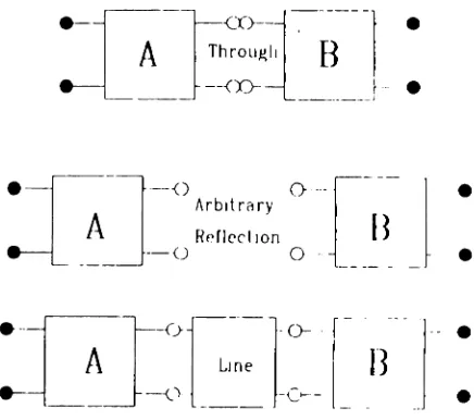
The s parameter measurement of an arbitrary t\VO port network can be divided into

two tiers. First we have the calibration of the network analyzer, i.e. measurement

and calculation of AN ..~ error terms, and second we need to interface our arbitrary

network to the network analyzer. This interface or adaptor is commonly referred

to as the fixture. For example, if we were interested in measuring the s parameters

of a microstrip transmission line we need a fixture to adapt from a coaxial AN A to

microstrip and then back again, Fig. 2.1.10. Fixturing introduces error into our

measurement and modeling and additional calibration measurements we can

re-move this error. This fixture calibration is sometimes referred to as de-embedding

because the device to be measured is embedded within the fixture. From this point

on the terms calibration and de-embedding will be interchangeable.

Fig. 2.1.11 shows the fixture error model. It is composed of two error networks

classical one port calibration, there are six independent error terms for this model

and we can use one port calibration standards to calculate them. This result is

accurate if forward and reverse transmission through the fixture are equal. Fig.

.:

Microstrip Line

Coaxial Reference Planes

, ,

, ,

:~

L

.:

,

.

" ' /

Microstrip Reference Planes

A

1

Line

₂

₈

Figure 2.1.11: Block diagram of a two port fixture, A and B contain the fixture error networks and the measurement planes are fixture ports 1and 2.

~----I----"---'-"""""""----+---,

e'Ob

rule verifies this fact. In general, a fixture is passive and non magnetic therefore

must have equivalent forward and reverse transmission coefficients. This is the

only difference between Hackborn's AN A two port error model and the six term

fixture model. The ANA, however , can only be minimally modeled by the eight

term two port model. Additionally, fixtures can be constructed such that port to

port coupling is much smaller than that internal to the AN A and we do not need

to modify the fixture error model. The disadvantage with fixture de-embedding

is that its geometry can be very different from one port calibration standards

discussed above.

Unfortunately many fixtures encountered in microwave measurement can not

use the classical one port calibration standards and there exits a need for unique

two port fixture standards or de-embedding standards. To strengthen this point,

consider a microstrip fixture. We have seen that it is advantageous to use a

matched load standard since it allows direct measurement of one error term. This

of course assumes we know its reflection coefficient. In microstrip we can not

fab-ricate an effective matched load and a sliding termination is physically impractical

so we must 1)se other stanrIa r d s. Sirnl1c:l rlv a n open r irr-n it. ~1a n

n

a rrl is rli ffir ulf t.o

line of different geometries.

By

measuring our fixture with a known two port

(transmission line) inserted between the fixture error networks we introduce a

distributed de-embedding standard.

In 1975 Franzen and Speciale introduced distributed standards for calibrating

their AN A. Although their result is not a two-tier approach it is significant

be-cause they were the first to introduce distributed standards. Their technique was

conveniently called Through-Short-Delay or TSD

[18].

At this point we would like to briefly outline the next discussion of various

fixture calibration procedures. First \\Te will look at the standards used and

con-sider the authors motivation and second we will examine the disadvantages we can

encounter when using them.

TSD - Through-Short-Delay

TSD is based on both reflection and transmission measurements and it ()rrer~ f\YO

advantages. First, a matched load standard in not required and second it uses

mechanically simple standards. In addition, Franzen and Speciale found that an

TSD is not without disadvantage. The delay standard was assumed lossless and

nonreflecting i.e. the propagation constant was pure delay and the impedance was

that of the measurement system or 50 ohms. Also, TSD although not mentioned

by these two, requires information from two delays; the through connection and

the actual delay. If the phase difference between these two is near zero or 180

degrees the algorithm will fail to return a valid result. This is a limitation of any

de-embedding technique that uses a delay type standard. Franzen and Speciale did

not apply their results to a planar fixture but their work is significant. In 1976,

Bianco et al. considered the planar problem first hand by applying distributed

standards to a microstrip fixture

[19].

Line-Offset Open-Line

Bianco used a total of three distributed standards; two delay lines and one offset

open circuit for de-embedding standards. Just as with TSD, the delay lines were

nonreflecting but they were not assumed lossless, in fact, the propagation constant

and open circuit reflection coefficient could be determined for the microstrip line.

The mechanics of their de-embedding required a separate measurement for each

inserted delay line and a one port measurement with the error networksterminated

with the offset open circuit. Of course their algorithm was subjected to the 180

degree bandwidth limitation wit h an added problem. When two delays are used

it is assumed uniform and they have equivalent characteristic impedances. It is

connection and an arbitrary reflection to calibrate their network analyzer. The

delay standard could be arbitrary, that is, its propagation constant need not be

known, however, the line was assumed nonreflecting. The reflection standard

could be any repeatable reflecting load and they suggested either an open or short

circuit. Again, this result was stated by Bianco but Engen was the first to consider

algorithm singularities associated with distributed standards.

Neither the Bianco or Engen work had been applied directly to a fixture.

Benet, in 1982, introduced the universal 1\f11IC test fixture that required

sev-eral distributed standards for calibration yet they chose yet another calibration

algorithm.

Open-Short-Five Offset Lines

Benet developed the open-short-five offset line calibration using a one tier

ap-proach [21]. As discussed before, the one tier calihratioll is usually n'IItnl'" Oil

the twelve term AN A error model, that is, six for each direction of measurement.

To determine the six terms Benet measured the fixture's response with open and

short circuits at the fixture reference plane and then a minimum of three offset

additional error term. Two additional offset lines were used to allow a least squares

fit of the circle to these measurements. Returning to the open and short circuit

error equations, he showed that two additional error terms could be determined.

Finally, by approximation he determined the propagation constant of the thru

lines and the remaining error terms. Benet's contribution showed that insertable

distributed standards could be used to calibrate a test fixture. Next we will see

that a two tier de-embedding method obtains a similar result and requires fewer

assumptions.

Open-Short-Modeled Through Line

Under some circumstances the fixture can not be calibrated using insertable

stan-dards such as a transistor test fixture. Here the fixture can not be separated

to insert the de-embedding standards. In 1982 Vaitkus and Scheitlin proposed a

method of de-embedding such a fixture by considering a two tier de-embedding

method. The AN A was first calibrated using OSL and its twelve term error model

and then fixture de-embedding measurements were done. Their standards were

an open and short circuit and a modeled through line [22]. The error model was

simply a one port error network for each fixture port and tV-TO leakage terms to

compensate for a leakage path around the transistor chip. This is a simplification

of Rehnmark'8 ten term AN A error model. Vaitkus and Scheitlin exploited the

A through line standard had been previously used by others but Vaitkus

dif-fered by using a modeled through line and determined its equivalent circuit by

optimization. A bond wire through line connected the fixture ports together and

the equivalent circuit was optimized to fit the measured fixture s parameters.

A similar procedure was performed on the bond wire short circuits. Vaitkus and

Scheitlin produced results using a through line standard but a general examination

of Open-Short- Through line was introduced later by Vaitkus himself [23] in 1986.

Rather than model the through line, he assumed knowledge of line propagation

constant, short circuit inductance, and open circuit capacitance.

Double Through Line

In 1987, Pennock et al. introduced a de-embedding technique for characterizing

transitions between novel transmission media

[24].

Their motivation was a lack of conventional standards and a need to reduce the tot al ueedvd. In 1!ri(i, I~i(tfH"O ct

ale eluded to the fact that transition parameters could be determined to within a

multiplicative constant if only two through line standards are used [19]. They also

showed that measurement of an additional through line was a linear combination

the multiplicative constant and proceeded to use two line standards for their

de-embedding.

Their fixture error model was the commonly used six term two port error model

and we know that to completely characterize it we need three standards. Pennock

showed that the Bianco constant was a ratio of two error terms. In fact, this

ratio is nearly equal to unity for reasonable transitions and Pennock proceeded to

de-embed the fixture under this assumption.

This result is not without problems. First, as stated before distributed

stan-dards must avoid

>../2

singularities and second, the line must be reflectionless.

Additionally, the line attenuation constant is known or assumed equal (lossless

line) .

TTT - Triple Through

In 1988, Meys introduced a fixture de-embedding method that uses an auxiliary

two port and matched load for standards [25]. Beginning with the standard two

port error model, the

A

and

B

error networks are connected together and

mea-sured. Also, the auxiliary two port C is cascaded to either side of

A

a nrl

n

t.o

form the measured two ports Be and CA. These and the AB t\VO port provide

necessary but not sufficient information to determine the error networks. TIle

reflection coefficient for the auxiliary two port terminated with a matched load is

sufficient to determine the error networks.

Results of Eul and Schiek

In 1988, Eul and Schiek examined the conventional two port measurement system

from a linear algebraic point of view. Their worked showed results noted by

previ-ous authors such as a need for at least three de- embedding two ports for complete

characterization and previous de-embedding techniques. Their main contribution

was the study of redundancy [26]. When three standards are inserted between the

error networks and subsequently measured, the total number of unique measured

quantities is twelve, yet there are only eight error terms linearly independent.

This redundant information can be used to reduce the required knowledge of the

standards used and as a result they proposed several de-embedding methods

Thru-Match-Reflect is one example.

TMR - Thru-Match-Reftect

Thru-f'vlatch-Reflect uses a through connection, a matched luad (Of any other

known reflection coefficient) and an arbitrary reflection. It offers the broad-band

advantage of these standards however we need a prior knowledge of at least one

standard i.e. the matched load. The reader is referred to [26] for discussion of the

2.2

Conclusion

The review of calibration theory encompassed one port measurements, automatic

network analyzer error models and calibration methods and finally fixture

de-embedding. It is clear that calibration of network analysis has been an ever

chang-ing study coverchang-ing much of our recent history. It contains a variety of methods

because the results of one may not be applicable to another or someone has a

unique de-embedding requirement. It is important to note that when

approach-ing a calibration dilemma one should look at the problem from a know / unknown

point of view. In other words, consider the total number of unknowns in the

mea-surement system and then decide on the variety of standards that are available.

We feel that this review has provided the insight into calibration methods and

hopefully given the reader a "what if we use ... " attitude towards their calibration

of network analysis. The next chapter approaches new calibration methods and

3.1

Introduction

As we have seen from Chapter2, it is clear that a calibration can take many forms.

Naturally, we feel that another calibration topic remains untouched; exploitation

of the symmetrical nature of measurement fixtures. As with past calibration

meth-ods, there was a need for something "new" and we are similarly motivated with

this study.

Chapter 3 concentrates on discussing advantages of symmetry arguments,

re-viewing symmetrical de-embedding methods, and the development of two new

symmetrical de-embedding algorithms. In addition, we will re- examine TRL

cal-ibration and develop a practical enhancement.

3.2

Motivation for Using

Syrn

met r ical Argurnent s

When considering the history of calibration of network analysis, two directions

have been pursued by the measurement community. On one hand, there was a

need to compensate for imperfections in calibration standards, and on the other

at all possible choose the minimum necessary. A symmetrical argument allows a

reduction in required standards thereby improving the certainty. In fact, later in

this chapter we show that it is possibly to reduce the total number of standards

to one. With this in mind, when can we use a symmetric argument or when is a

fixture symmetric?

3.3

Evolution

frorn

an

Asyrn

met r-ic

to Symmetric Fixture

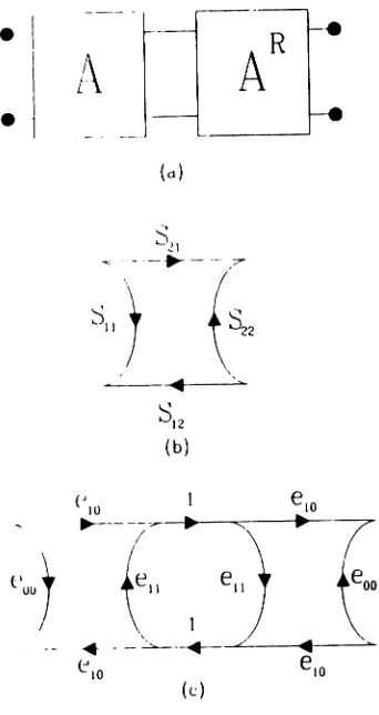
A symmetric fixture is a special case of the general asymmetric fixture. In Fig.

3.3.1, we see the conventional two port error network and its corresponding signal

flow graph. It is composed of two error networks A and B and in general, the

individual signal paths

5

i j a and

5

i j b are unique forcing fixture s parameters

5

i j /

to be unequal to each other. This represents an asymmetric fixture.

A fixture is symmetric if the port 1 and 2 reflection coefficients are equal and

the fixture is reciprocal, i.e. if 51 1 /

==

52 2 / and 52 1 /

==

51 2 / . Reciprocity is true

when the fixture is passive and non-magnetic and these symmetrical equalities are

possible with two orders of symmetry; first and second order.

are related to the individual error terms,

S

-

C'

S21a Sl2a S

l l b

11J - ,,"711a

+

1 S S

- 220 lIb (3.3.1)

•

e-

B

-.

.,

~Il

t

/

---.--~

Sl2

(b)

e

l Oa 1

e

Ol b

~.--~. '<, •

-eoo)

(ell.

I

ell)

t

O

O

h

~~ ~- < ~ ~

e

_{Ol a}

e

_{l Ob}

(c)

Figure 3.3.1: Two port error model for an asymmetric fixture (a). Fixture error can be described with eight error term SijQ and Sijb. Port 1and 2 are the calibrated

and

S_{12/ =} S12aS12b

1 - S22aSl l b

(3.3.3)

(3.3.4)

Equating 3.3.1 and 3.3.2 and applying reciprocity we find one equation in six

complex unknowns.

(3.3.5)

This is the symmetry condition equation representing an under determined

sys-tern. This implies that symmetry can be produced with an infinite number of six

error parameters. Fortunately, symmetry corresponds to the physical nature of

the fixture which limits the symmetric solutions to two; first and second order

symmetry.

3.3.1

First Order Syrn met r ic Fixture

A first-order symmetric fixture has identical fixture halves that are asymmetric,

see Fig. 3.3.2. The port two error network, B, is now a port reverse of

A,

or

c;'} ~[. ,r ('( )vf'r

I 2II,' 1\ ,

these conditions satisfy the symmetry condition equation 3.3.5. A "coaxial to

rTll-crostrip" - "microstrip to coaxial" fixture is an example of first order fixturing.

Most important, the signal flow graph shows that the symmetry reduces the

•

•

(0)

•

e_{l O} 1

e

_lo

~---.-

•

""

•

₇

I

I

(. 7

_uu

_\~Il

ell

\00

.-

--~--+- <' _{~ " "}

-t'10 e,o

(c)

Figure 3.3.2: Two port error model for a first order symmetricfixture (a). Fixture error networks are described

by

three s parameters Sija. 811J and 821J are the

allows a reduced number of error terms for a two port fixture, and this reduction

is strictly a function of the manufacturing repeatability with direct application to

printed circuit board measurements.

3.3.2

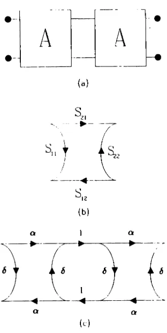
Second Order Symmetric Fixture

If the fixture halves are identical and symmetric, the fixture is second order

sym-metric. This implies that network B is equal to A or all reflection s parameters,

Su;

or

5

ii b , are equal,(

=

51 1 ) and all transmission s parameters are equal, Sija or

5

i j b ,

(=

52 1 ) , see Fig. 3.3.3. A second order fixture satisfies the symmetry condi-tion equacondi-tion 3.3.5 and a lumped element transistor test fixture is an example of

second order fixturing.

3.4

Review of Syrnrnet r ical Methods

Previous authors have examined symmetric fixtures. In 1982, Souza et. al. used

a rnicrostrip first order fixture to develop a method to calculate the fixture half.

Their results are based on further assumptions. First, the microst rip line used

fixture half has a low return loss [27J. However, this result can not be applied to

a fixture that introduces significant error. If the fixture microstrip line impedance

is different from 50ohms, both assumptions are invalid.

e-

••

A

A

e-(0)

s,

H _ ~_ _ _ _ _ _ _

, I

SII}

(~2

~._--.-~

S12 (b)

Q' Q

.- -

.----;;--6

(6

IJ

{6

1 _,

. / ~ ~ _~ . /

~

a Q'

(c)

Figure 3.3.3: Two port error network for a second order symmetric fixture. Fixture

by modelling their fixture half with a pi equivalent circuit with different shunt

capacitances

[35].

Their calibration standards are an open and short circuit and a through connection. The fixture input impedance equations for the open and

short standards give sufficient information to extract the pi equivalent parameters

if second order frequency terms are neglected. As with the Souza result, they use

assumptions in addition to symmetry. Their result is invalid when the fixture is

considerably long or can not be modeled with a lumped element circuit. In 1986,

Ehlers was the first to apply symmetry without additional fixture assumptions.

Ehlers studied a finline first order symmetric fixture. The standards include

a through connection and either a matched load or a reflectionless transmission

line

[37].

He pointed out that a symmetric fixture requires two standards for cali-bration. This is true only if the matched load or a reflectionless transmission line

can be fabricated.

If

neither are accurately possible (as is the case for microstrip

fixtures) then an additional standard is needed. For the finline example his result

is adequate.

Most recently, In 1989, Enders developed an iterative de-embedding method

that uses three line standards to determine the pararneters of a first order fixture

[36].

His result affirms the belief that symmetry is useful for calibrating fixtures and in the next section we will apply symmetrical arguments and distributed

cal-ibration standards. A second order fixturing was examined

by

Martin and

3.5

Development of Through-SYlllmetry-Line - TSL Using

First Order Symmetry

3.5.1

TRL to TSL

As we have seen before, the calibration of a planar measurement fixture, e.g.

microstrip and stripline, requires distributed standards. The preferred method

for planar fixture de-embedding is Thru-Reflect-Line (TRL) or Line-Reflect-Line

(LRL) because the distributed standards are easily modeled and constructed. A

typical microstrip fixture, shown in Fig. 3.5.1, is a first order symmetric fixture.

Identical coax to microstrip transitions and identical microstrip line lengths are the

requirements for symmetry. These can be achieved into low microwavefrequencies

and at higher frequencies through careful design.

Because first orrler svrnrnetrv allows 1he fixtnre to he rpprpsentpd 'Ylfh fhrpp

error terms, three standards are needed. Symmetry permits synthesis of 'I'Rl,

reflection standards thereby eliminating their need. TRL standards are shown

in Fig. 3.5.2; through connection, an reflection and a reference transmission line

Ground Planes

I

'

Embedded - ....~ Microstrip

Une ,

:~

L

=

348 mils

L

=

1348 mils

(a)

Coaxial Reference Planes

8M

..

QJ. ..

~ MicrostriP~"

Q.? ..

A

~

Reference Planes

M1

M2

Vi

(b)

e

h

AJ-("">-1~:n~1-~ r~

B

--(")

-c~-- -c~-- - - -

---

.

•

symmetrical through connection, we can calculate the reflection coefficient with

the microstrip ports terminated in ideal open or short circuits. Either synthesized

reflection coefficient can be applied to the TRL algorithm. Conforming to the

naming of de- embedding methods we will refer this substitution as

Through-Symmetry- Line or TSL.

3.5.2

Synthesize Reflection Standards

The TSL standards are a through and line connections, Fig. 3.5.3. These are

similar to Souza et al.

[27]

however their result is based on symmetry and a low fixture return loss assumption. Note, the symmetry reflection coefficients can

be used with the LRL algorithm with similar results. Next we will expound the

derivation of ideal open and short circuit reflection coefficients.

Referring to the signal flow graphs of Fig. 3.5.4, we consider the through

connection 5 parameters given by, 51 1 / (

==

52 2 / ) and 521 / (

==

51 2 / ) , and the actual

parameters of the A network being

0,

Q and 1 for 51 10.,52 10.

==

5

120. and

5

220.

respectively. In addition, the input reflection coefficient with an ideal short circuit

placed at port. 1h of A is

(3.5.1)

Before we used Mason's rule to relate the fixture parameters to the individual

.--A

.---.

B

Through

(a)

:G

:J~D

Delay

t:r

B

t:

(b)

Figure 3.5.3: TSL calibration standards. (a) Through connection and (1») Line

•

r--~\

_A

R

10..

_~, Jb _~

•

J--

-.

(a)

0(.

~--;-I

r

'(I

J

t

\

(b)

S.?I

-:.. - - - -.- - - / 7

~ ~

(-..

, II ) :)22

I ~

">

SJ2

(c)

Figure 3.5.4: TSL signal Row graphs. (a) Measured fixture s parameters,

(1))

Combining (3.5.1), (3.5.2) and (3.5.3), the short circuit reflection coefficient can

be expressed as a function of fixture s parameters (measured).

(3.5.4)

A similar results holds for an ideal open circuit placed at port 1b.

(3.5.5)

Naturally, TSL can reduce the number of standards needed and requires fewer

connections to the microstrip ports improving the repeatability of this

connec-tion. Moreover, Pae and Poe can be derived for any fixture that exhibits first or

second order symmetry including other planar measurement fixtures. Since these

reflection coefficients are derived mathematically, it is possible to "insert" ideal

open and short circuits within a non-insertable medium such as a dielectric loaded

a symmetrically synthesized short circuit. In the next section will discuss an

3.6

Enhanced Through-Symmetry-Line - ETSL (ETRL)

3.6.1

Motivation: Failure of

TRL Assumpt ions

The development of ETSL, hence ETRL, is necessary because of assumptions

inherent to the TRL algorithm. As introduced in 1979 by Engen and Hoer [20],

the algorithm requires the characteristic impedance of the line standard to be

equal to the measurement system impedance. If not then we its value has to be

determined. Also, the algorithm assumes a pure real characteristic impedance with

no frequency dependence. If the fixture to be calibrated is composed of dispersive

transmission lines, e.g. microstrip, it becomes necessary to determine the complex

characteristic impedance

Z;

as a function of frequency. We present a method

that enhances the TSL algorithm by determining the characteristic impedance;

Enhanced Through-Symmetry-Line - ETSL. For the sake of discussion we will

consider an embedded rnicrostrip fixture. Application of ETSL to an embedded

microstrip fixture follows in Chapter 5.

An approximate value of

Z;

can be made USIng time domain reflectometry

(TDR), however, TDR can not determine frequency variations of the microstrip

characteristic impedance which can vary by as much as 5 percent from DC to 10

GHz

for a typical rnicrostrip line [32]. Also, accurate modeling of Z; is complicated

by several factors; accepted models predict different frequency variations; material

experimentally determined propagation constant, ,

==

a

+

jj3.

The impedance calculated in this fashion, if used in the conventional TRL algorithm, compensates for the algorithm assumptions. By using a free-space

capacitance explicit knowledge of the dielectric parameters i.e. relative dielectric

constant and loss tangent are not necessary. Also, we can determine characteristic

impedances of geometries that are atypical such as embedded rnicrostrip or any

uniform TEM transmission line. Additionally, by incorporating the propagation constant we embody the effect loss has on the characteristic impedance (complex

Zc).

In short, this method can be used to determine characteristic impedances of

any arbitrary uniform

TErvI

transmission line. In the next section we will develop

the characteristic impedance algorithm with microstrip being the transmission

line.

3.6.2

Calculation of

Corn plex

Characteristic Impedance

Microstrip lines are non-homogeneous transmission lines that support. a

f)11~~1-TEM mode [32]. However the TSL algorithm requires the equivalent TElvl mode

characteristic impedance. For uniform TE1'1 transmission lines the characteristic

Dielectric Thickness H

=

5.6 mil

t

_t

Microstrip Width

=

8. mil

[§]

Solder Resist Layer

D

Substrate Dielectric • Metal (copper)

GP Thickness

=

1. mil

Figure 3.6.1: Embedded microstrip encountered in printed circuit board

1

Zo= =

-Coc

(3.6.2)

where Z; is the dielectric loaded characteristic impedance of the line, Zois its

free-space characteristic impedance,

Co

is the free-space capacitance, c is the velocity

of light and f_e is the effective dielectric constant.

Co

is a geometrical dependent

factor and is the capacitance of the structure in a dielectric-free medium. It is well

known that the effective dielectric constant is related to the propagation constant

, by [28]

(3.6.3)

where, == a

+

j(3 is available from measurement as a by product of the TRL

algorithm. Recently, Mondal and Chen reported that the TRL algorithm can be

used to determine the propagation constant of the TRL line standard. That is

[29]

where

A

== TIlt· T221

+

TIll· T22t - T21t •TI21 - TI2t .T21 ,

(3.6.4)

(3.6.5)

Tijl and Tijt are the chain scat tering parameters for the line and through cali

from s to t parameters is given by,

(3.6.6 )

where

(3.6.7)

This result can be derived for any fixture, symmetric or otherwise, and it is a

nat-ural progression to incorporate this information to determine the complex

charac-teristic impedance. Combining (3.6.1)- (3.6.3) and taking the negative root

JW

z,

== ~C

c

0,

(3.6.8)

The negative root is chosen because the result must be positive when the line is

lossless and the impedance is positive pure real. This characteristic impedance is

used to overcome impedance assumptions of TRL and is applicable to the TSL

algorithm. The reader is directed to Chapter 5 where this derivation is

experimen-tally verified with a fifty ohm coaxial example. Also, Chapter 5 contains complex

rnicrostrip characteristic impedance calculated with the verified algorithm. Next

we examine singularities that arise when distributed standards are used and

ex-pand on the effect these singularities have on calculating tlie propagation rf)ll~f;'l1f.

3.6.3

Calculation of Propagation Constant

Inherent to the TRL algorithm is the need to separate the error networks with a

mea-degrees it appears transparent. TRL returns invalid results in either case.

In-tuitively the "farthest" we can be from 180 degrees (or zero) would be a phase

difference of 90 degrees and reliable propagation constants can be extracted from

20 to 160 phase differences [30]. By choosing line standards with electrical lengths

within this range the characteristic impedance can be determined with no effect

from the singularities.

3.6.4

Modifying TSL Algor

it hm

Again, the TRL (TSL) algorithm requires a reflectionless line. This is achieved

by transforming each calibration measurement from the measurement reference

impedance to

Zco

Application of TRL then determines the S parameters of the

er-ror network referenced to

Zc.

To complete calibration the s parameters of the error

network are returned to the measurement reference impedance system, (usually

3.7

Development of Through-Symmetric Fixture - TSF

U sing Second Order Symmetry

What

if

the fixture is second order syrnmetric? Again, we define second order

symmetry as a first order fixture with symmetric halves. As we have just seen,

symmetry can be used to reduce the number of standards needed. When second

order symmetry is valid the two port error network is represented with two error

terms. Naturally, this allows us to use fewer de-embedding standards, in fact, a

second order fixture requires only one measurement configuration, a through

con-nection, thus in conformance with the practice of naming calibration procedures,

we designate the new technique Through Symmetric Fixture - TSF method.

Fig. 3.7.1 shows the signal flow graph for the fixture s parameters SiiJ and

the corresponding two port error model. Each error is identical and symmetric

therefore the scattering matrix of each is

b Q

[Sija] == (3.7.1)

Q 6

The goal of TSF is to determine the error terms(Q a nd

6)

and based on M ason 's

non-touching loop rule, unlike the matrix renormalizations used by Mar tiu c\11(1

Dukeman [31].

S

parameter measurements of the through connection yield t\VO

independent quantities, 5u / and 521 / , as 5u /

=

522 / and 512 /

=

521/ because of

symmetry and reciprocity. This is sufficient to determine

5

i j a • For clarity, we will

•

•

A

(a)

S~I

<, - - - . .

-/

~

I I , '

t

i~·

\::i

a

- ' - - -_ _~_ _- A .

Sl2

(b)

-

.

-

.

(c)

The signal flow graph provides two algebraic relationships for the known qu a

n-tities as functions of the error terms

_,

Rearranging

0:2

S_{21t -}- - -_{1 _ 6}

2

(3.i.2)

(3.i.3)

(3.7.4)

where

Q== (3.7.5)

b== 1

+

S21t (3.7.6)

The square root gives t\VO possible solutions and the root choice depends upon the

electrical length

(L

e ) of the through connection. The positive root is valid when

where

(2n

+

l)A

nA

<

L;

<

-2

n == 0,1,2, · ..

(3.7.7)

(3.7.8)

otherwise the negative root is correct. This choice of roots is based on (l

1"'.'

sical

constraint. The a term is the transmission coefficient of the error network and at

low frequency the phase of Q must be negative therefore the positive root choice

length of the fixture is constructed such that it is not an integer half wavelength

long at any frequency in a desired measurement range. TSF can be used on a

lumped-element transistor test fixture "There this restriction does not exist.

Sim-ilar singularity restrictions exist when other distributed de-embedding techniques

are employed. The reader is directed to Chapter' 5 where

TSF

is experimentally

verified.

3.8

Conclusion

In Chapter 3, we have presented new de-embedding algorithms. By using

sym-metric arguments, it is possible to reduce the required calibration standards. It

was shown that reflection standards can be synthesized from a through

measure-ment. Also, the complex characteristic impedance of uniform TEM transmission

lines can be determined if the transmission line free-space capacitance is known.

T~kln~this irnperlance into ar cou nt . "?P r a n pnhf'nrp thp T~T,or TnT} tllgnrlihms.

Computer implementation of these algorithms is necessary for verification

pur-poses. The next chapter develops SPANA or Signal Processing of Automatic

Network Analysis a command level program useful for algorithm implementation

Chapter

4

SPAN A: Computer Program for Computer

Aided Microwave Measurement

4.1

Introduction to SPANA

Computer processing of microwave measurements is necessary to free the engineer

from the costly measurement time. It is very reasonable to assume that computer

processing is needed since a single t\VO port measurement can produce sixty four

kilobytes (64K) of data.

SPANA

(Signal Processing for Automatic Network

Anal-ysis) has been developed to meet the needs of automatic microwave measuring

systems.

SPAN A

is a tool to be used for processing measured S parameter data and its

prime use is to implement de-embedding algorithms. SPAN Aalso performs various

tasks such as input/output of data, data format conversions, and others. Written

SPAN A

is by the simplest definitions an operating system

and

the operations

are carried out by using a command language. These commands allow the user

to interact with the data freely. One of the most important assets of

SPANA

is