A two-scale model for an array of AFM
0
s cantilever in
the static case
M. Lenczner
∗and R.C Smith
†June 19, 2006
Abstract
The primary objective of this paper is to present a simplified model for an array of Atomic Force Microscopes (AFM) operating in static mode. Its derivation is based on the asymptotic theory of thin plates initiated by P. Ciarlet and P. Destuynder and on the two-scale convergence introduced by M. Lenczner which generalizes the theory of G. Nguetseng and G. Allaire. As an example, we investigate in full detail a particular configuration, which leads to a very simple model for the array. Aspects of the theory for this con&guration are illustrated through simulation results. Finally the formulation of our theory of two-scale convergence is fully revisited. All the proofs are reformulated on a significantly simpler manner.
1
Introduction
In recent years, a number of new Microsystems or Nanosystems Array architectures have been developed. These architectures include microcantilevers, micromirrors, droplets ejectors, mi-cromembranes, microresistors, biochips, nanodots, nanowires to cite only few and application are continually emerging in numerous areas of science and technology. In some of these systems, units have a collective behavior whereas in others they are working individually. However, in all cases their coupling is an important design parameter of the array that is promoted or avoided. The coupling can be of various natures including mechanical, thermal and electromagnetic. The numerical simulation of such whole arrays based on classical methods like Finite Element Methods (FEM) is prohibitive for today0s computers at least in a time compatible with the time scale of a designer. Indeed, the calculation of a reasonably complex cell of a three dimen-sional Microsystems requires about 103 degrees of freedoms which leads to about 107 degrees of freedoms for a 100×100 array. Moreover usual Microsystems involves strong nonlinearities that cannot be ignored.
This work is focused on a relatively simple example of Microsystems Array, namely an Atomic Force Microscopes Array (AFMA). A number of developments of AFMA or of more simple Cantilever Arrays have already been achieved, as noted in the abbreviated set of citations [29]-[62].
∗Center for Research in Scientific Computation, North Carolina State University, Raleigh, NC 27695. E-mail
address: [email protected].
†Center for Research in Scientific Computation, North Carolina State University, Raleigh, NC 27695. E-mail
The modeling of single AFM has been extensively studied in the literature in many different configurations, as noted in the review papers [14], [21] and [13]. Most of the models are based on a spring-damper-mass model where the precise features of the mechanical systems are ignored. More careful modeling has been derived in various situations including tapping mode, interaction with a surrounding fluid; see [16]-[23]. They are based on the Euler-Bernoulli beam model with an applied force at the extremity of the beam except in [12] where the tip is modeled as a rigid part and the force is applied to it. Until now, with the best of our knowledge, only the group of B. Bamieh, see [24] and the reference therein, has published a model of coupled cantilever array. These authors take into account the electrostatic coupling with a rudimentary derivation.
To simplify the discussion we focus on the simplest case of an AFMA in static operation. We establish a two-dimensional thin plate model for an elastic component including a rigid part corresponding to the tip that is assumed to be much stiffer than the supple part of the cantilever. Then a simplified model of an array of AFMs coupled through their base is derived from the thin plate model. Each of these models is illustrated by an example. Analytic calculations are conducted to yield very simple formulations. Finally a numerical simulation of the array is presented and discussed. The derivations of the two models are rigorously justified through asymptotic methods. The thin plate model is based on the asymptotic methods of P. Ciarlet [2] and P. Destuynder [1] as well as on our previous work [6]. The derivation of the AFMA two-scale model uses the two-scale transform and convergence introduced by one of the author, see [15], [11] and [10]. However it is completely reformulated in a simpler and more intuitive manner.
We note that for the geometry considered in this paper, our two-scale convergence is equiva-lent to the two-scale convergence of G. Nguetseng [7] and G. Allaire [5]. However it is worthwhile to remark that it has the of working also for electrical circuit homogenization (as a particular case of d−n dimensional periodic manifolds immersed in a d−dimensional space) when the other doesn0t apply as it has also been recognized in [9]. This remark constitutes an encour-agement to develop this method in the framework of Mechatronical Systems. We point out that these methods are in the vein of the homogenization methods by E. Sanchez-Palencia [3], L. Tartar and A. Bensoussan, J.L. Lions, G. Papanicolaou [4]. Finally, we cite the work of G. Griso and his coworkers initiated in [8] who have rediscovered the same method and named it the Unfolding Method.
one side a fourth order one-dimensional boundary value problem related to the deflection in the base coupled with the model of the cantilever at the micro-scale which reduces to a single nonlinear algebraic equation related to the tip-sample distance. The numerical simulations are conducted for simple sample profiles: flat, slope and a quadratic shape. The tip-sample distance is a distributed variable along the array that we discretize with Chebychev polynomials. The numerical experiments show that even for simple sample shapes, a relatively large number of polynomials are required for an accurate approximation. It is also observed that even for a moderate number of cantilevers the deflection of the base is far from being negligible in comparison with the tip displacement. This is due to the fact that the deflection increases when the length of the base increase as its fourth power.
We note that the derivation of a two-scale model for the evolution problem can be directly deduced from the static model. However the dynamic problem requires much dedicated analysis, simulations and discussions so that we have chosen to postpone its presentation until a further publication.
The paper is organized as follows. We establish aspects of the geometry and nature of tip forces in the remainder of this section. The three-dimensional elastic model coupled with a rigid part is stated and derived in Section 2. The thin plate model is stated and derived in Section 3. The two-scale model is stated and derived in Section 4. It is based on the two-scale theory presented in the appendix postponed in Section 7. The examples and the numerical simulations are reported in Section 6.
2
Three-Dimensional Model
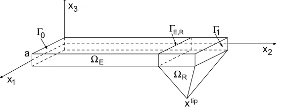
We start by considering a mechanical structure located in Ω ⊂R3 made up of an elastic part and a rigid part located respectively in ΩE and in ΩR as depicted in Figure 1. The model is
stated in the next section and subsequently justified in Section 2.2.
2.1
Statement of the Model
The elastic component is clamped along part of its boundary Γ0, is linked to the rigid part through the interface ΓE,R and is free of applied forces in the remaining part Γ1. When the
system is totally elastic (no rigid part), then ΩR and ΓE,R are void and the related equation
must be ignored. The mechanical displacements are denoted by the vector u = (u1, u2, u3)T defined over the entire structure.
a
x x1
x2 x3
Γ0
ΩE
E,R
Γ Γ1
R
Ω
tip
Figure 1: Three-dimensional plate with the rigid part
is the gradient operator. The equilibrium equations, the linear stress-strains relation and the rigidity constraint are stated as
−div(σ) =f, σ=Rs(u)in ΩE ands(u) = 0 inΩR (1)
where the product between the fourth-order tensorRand the matrixs(u)gives the3×3matrix with entries
σij =
3
X
k,l=1
Rijklskl(u).
In the case of isotropic elasticity, the elasticity tensor has the form
Rijkl=λδijδkl+ 2µδikδjl
where δ is the Kronecker delta.
The boundary conditions areu= 0onΓ0,σn= 0 onΓ1 (nbeing the outward normal vector to the boundary). Moreover, u will be continuous at the interface ΓE,R. Finally, the force and
force momentum transmissions satisfy
Z
ΓE,R
σ n ds=ξ,
Z
ΓE,R
(σ n).(x×ek) ds=Ξk for k ∈{1,2,3} (2)
where
ξ =
Z
ΩR
f(x)dx, Ξk=
Z
ΩR
f(x).(x×ek)dx.
We note that the condition s(u) = 0 can be formulated through imposing a rigid displacement
u=b+x×B whoseb andB are some three dimensional vectors. The variational formulation, which is necessary for the formulation of Galerkin-like numerical methods, can be formulated as follows: find u∈V such that
Z
ΩE
σ ::s(v)dx =
Z
Ω
f.v dx (3)
for all v ∈ V for the previous stress-strains relationship where the admissible space of test functions is
V ={v∈H1(Ω)3 / s(v) = 0 in ΩR and v= 0 on Γ0}.
The Sobolev space H1(Ω) is the set of square integrable functions inΩ, R
Ωv
2(x)dx <
∞,such that each component of their gradient are also square integrable.
2.2
Justification of the Three-Dimensional Model
Consider a sequence of elastic structures filling upΩso that its rigidity inΩRtends to infinity.
Namely, the sequence of elasticity tensors has the form Rn = R in Ω
E and Rn = nR in ΩR
where n varies in N∗ from one to infinity. The variational formulation of such a sequence of
elastic problem is as follows: find un∈VE
Z
Ω
[Rns(un)] ::s(v) dx=
Z
Ω
for allv ∈VE where
VE ={v∈H1(Ω)3 / v= 0onΓ0}.
Using classical estimates, one may prove that ||∇un
||2
Ω andn||s(un)||2ΩR are bounded uniformly
with respect to nwhere ||v||2
Ω = R
Ωv
2(x) dx.
The uses of theses estimates justifies the expansion un =u+O(1/n) with u independent of
n and satisfying s(u) = 0 in ΩR and s = s(u) in ΩE. Taking n to infinity in the variational
formulation and posingv= 0inΩR,it follows thatusolves the variational formulation (3). The
derivation of the local form of the variational formulation (3) is a routine and is not detailed here.
3
A Thin Plate Model
The cantilever of an AFM is comprised of a thin plate equipped with a tip as depicted in Figure 1. The thin plate is assumed to be elastic and the tip is modelled by a rigid body. A simplified model, based on the classical Love-Kirchhoffelastic thin plate theory, is stated in the forthcoming section and its justification is made in Section 3.2.
3.1
Statement of the Model
Because the elastic component is a thin elastic plate with thickness 2a and mean section ωE;
we consider the domain
ΩE ={x∈R3 /(x1, x2)∈ωE, −a < x3 < a}. (4) The three parts Γ0, Γ1 and ΓE,R of its boundary are parameterized in a similar manner by
referring to the corresponding boundariesγP0,γP1 andγPE,RofωE.The rigid part is parameterized
as
ΩR={x∈R3 / (x1, x2)∈ωR with−h(x1, x2)< x3 < a}. (5) When a is small enough the three-dimensional model can be simplified to a thin plate model. To justify it, we make some assumptions on the order of magnitude of the applied forces with respect to the thickness a:
fα=1,2 =O(1), a−1f3 =O(1)inΩ anda−1h=O(1)in ΩR. (6)
It then follows that
uα=uPα +O(a) andau3 =auP3 +O(a) inΩ (7) where O(a) is any vanishing quantity when a vanishes and uP satisfies the Love-Kirchhoff
kinematic relations
∂3uP3 = 0, u
P
α =u
P
α −x3∂xαu
P
3 with ∂3uPα = 0 forα = 1,2 inΩE.
In this paper, we neglect the contribution of the membrane displacementuP so we state only the model satisfied by the transverse displacementuP
3. It is governed by the equilibrium equations, the stress-strains relations and the rigidity constraint
div(div(MP)) = fP +div(gP), MP =RP∇∇TuP3 inωE anduP3 =b
P +BP.x inω
where
gPα(x1, x2) =
Z a
−a
fα(x)x3 dx3 andfP(x1, x2) =
Z a
−a
f3(x) dx3 inωE. (9)
In the case of isotropic materials, the elasticity can be formulated as
RPαβγρ=a3(
4λµ
3(λ+ 2µ)δαβδγρ+ 4µ
3 δαγδβρ). (10)
In addition, x= (x1, x2)T,bP is a scalar and BP is a two-dimensional vector. The boundary conditions are
uP3 =∇uP3.n = 0 onγP0 (11) andnTMPn= 0, ∇(nTMPτ).τ+div(MP).n=gP.n on γP1
where n and τ are the unit outward normal and the unit tangent to the boundary of ωE.
The transmission condition at the interface γE,R results from the continuity conditions of the
displacement uP
3 and of its gradient ∇uP3 and the continuity of the normal stresses. These can be expressed as
bP =|γE,R|−1
Z
γE,R
(uP3 − ∇uP3.x)|ωE ds,BP =|γE,R|−1
Z
γE,R
(∇uP3)|ωE ds (12)
−
Z
γE,R
div(MP).n ds=ξP and
Z
γE,R
nTMP −(div(MP).n)x ds =ΞP
where
ξP =−
Z
γE,R
(gP.n)|ωE ds+
Z
ωR
fP dx, ΞPα =−
Z
γE,R
(gP.n)|ωExα ds+
Z
ωR
fPxα−gαP dx,
|γE,R| denotes the length of the interface γE,R, gP and fP having been defined in ω
E and are
defined in ωR by
gαP(x1, x2) =
Z a
−h(x1,x2)
fα(x)x3 dx3 andfP(x1, x2) =
Z a
−h(x1,x2)
f3(x) dx3 inωR.
The variational formulation associated with this model is
uP3 ∈V
P
and
Z
ωE
MP ::∇∇Tv dx=
Z
ωP
fPv−gP.∇v dx for allv∈VP (13)
taking into account the stress-strains relation. The set of admissible transverse displacements is
VP ={v∈H2(ωP)/ ∇∇Tv= 0in ωR andv= 0on γP0} and H2(ω
P) being the set of square integrable functions on ωP so that their first order and
second order derivatives are also square integrable.
Remark 1 For the derivation of the two-scale model, we need an extension of this model for plates with varying thickness, namely, when ΩE and ΩR are replaced by
ΩE = {x∈R3 / (x1, x2)∈ωE and −k(x1, x2)< x3 < k(x1, x2)} ΩR = {x∈R3 / (x1, x2)∈ωR with−h(x1, x2)< x3 < k(x1, x2)}
where k is a positive function so thata−1k =O(1). In such a case, the model remains the same
3.2
Justification of the Thin Plate Model
The justification of the thin plate model is based on the asymptotic method of P.G. Ciarlet [2] and of P. Destuynder [1]. In these works, the thin plate model is derived for isotropic elastic bodies by calculating the asymptotic behavior of the elasticity system and of its solution when the parameter a vanishes. In this work we use the same method but our derivation is based on the paper E. Canon and M. Lenczner [6] where material anisotropy was encompassed. The only difference between the new model and that in [6] comes from the presence of the rigid body which does not significantly affect the proofs. Hence we report only the main steps in the calculations.
Since the asymptotic method consist of finding the limit whenavanishes, it is mandatory to introduce a scaled domain independent ofa and to formulate the problem on it. To do so, one introduces the change of variable Fa defined on Ω by Fa(x) = (x1, x2,1ax3) in Ω. The image
Fa(Ω) is denoted by Ωe and there the coordinates are ex = Fa(x). The whole model is now
expressed on the dilated domain. All variables or fields related toΩe are covered by a tilde. The rigidity, the mechanical displacement and the forces are scaled in different manners
e
R(xe) =R(x), eu(ex) = (u1, u2, au3)(x), fe(ex) = (f1, f2,
1
af3)(x) for x∈Ω.
From the assumption made on f, it is clear that||fe||eΩ is bounded. We also apply a scaling to the test functions
e
v(ex) = (v1, v2, av3)(x).
For a given displacement field v, define the 3×3 matrice K(ev) such that Kαβ(ev) = sαβ(ev),
Kα3(ev) =K3α(ve) =a−1s3α(ev)andK33(ev) =a−2s33(ev). Applying the variable changeex=Fa(x) in (3) yields the following variational formulation: find ue∈Ve such that
a
Z
e
ΩE
e
σ ::K(ev)dxe=a
Z
e
Ω e
f(xe).ev(xe) dex (14)
for allve∈Ve whereσe=RKe (ue) and
e
V ={ev∈H1(Ωe)3 / K(ev) = 0 in ΩeR andev= 0 onΓ0e }.
By equating ev =u,e one may prove that ||eu||eΩ and||K(ue)||eΩ are O(1)with respect to a. Thus we are led to formulate
e
u=ueP +O(a), K(ue) =KP +O(a)
where euP and KP are independent of a. It follows that
KαβP =sαβ(ueP) for α,β = 1,2 and that si3(euP) = 0 for i= 1,2,3. This is equivalent to saying that euP fulfils the Love-Kirchhoff kinematics
∂ex3eu
P
3 = 0 andeu
P
α =eu
P
α −xe3∂xαeu
P
3 with ∂xe3eu
P
α = 0.
e
uP3 ∈V
P
,
Z
ωE
f
MP ::∇∇Tve3 dxe=
Z
e
Ω e
f3 ev3−ex3feα∂xeαve3 dxefor allev3 ∈V
P
.
Here MfP =ReP
∇∇TueP
3 and ReP is defined under the name Q22 in E. Canon and M. Lenczner [6] and is equal to
e
RPαβγρ= 4λµ
3(λ+ 2µ)δαβδγδ + 4µ
3 δαγδβρ
in the case of an isotropic material. Applying the inverse variable change, uP
3 solves the varia-tional formulation: find uP
3 ∈VP such that
Z
ωE
MP ::∇∇Tv3 dx=
Z
Ω
(f3 v3−x3fα∂xαv3)dx
for all v3 ∈ VP with MP =RP∇∇TuP3 and RP =a3ReP. This leads directly to the variational formulation (13). Since ∇∇Tv3 = 0in ΩR it may be written v3 =d+D.xwith D= (D1, D2)T thus the right hand side may be reformulated as
Z
ωE
(fP v3−gP.∇v3) dx+ξPdP +ΞP.DP.
Application of twice Green formula and using the fact that v3 = d+D.x on γE,R, it follows
that
Z
ωE
div(div(MP)v3 dx+
Z
γ1
(nTMP∇v3−div(MP).n v3) ds
−(
Z
γE,R
div(MP).n ds) dP + (
Z
γE,R
(nTMP −div(MP).n x) ds).DP
=
Z
ωE
(f3P +div(g
P
))v3 dx−
Z
γ1
gP.n v3 ds+ξPdP +ΞP.DP
from which we deduce all the model equations excepted the continuity condition of uP
3 and
∇uP3 that comes by integrating the expressions uP3 =bP +BP.xand∇uP3 =BP on γE,R.
4
Model for an AFM Array
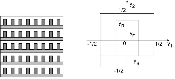
Consider a mechanical structure made of a periodic distribution of microcantilevers as shown on Figure 2. In Section 4.1 a simplified model is stated when its derivation is done in Section 4.2.
4.1
Statement of the Model
The whole domain occupied by the cantilever array is still denoted by ωP and is assumed to
0
B
y
F
y
R
y 1/2
-1/2 1/2
-1/2
1
y
2
y
Figure 2: Array of cantilevers and their reference cell
The dilatation and shift of any cell Yε
i gives rise to a reference unit cell Y ⊂ (−
1 2,
1 2)
2. For the derivation of the array model, we assume that ε/L1 << 1. As ωP, this microscopic cell is
comprised of a thin elastic plateYE and a rigid partYR.In YE, we distinguish the baseYB and
the elastic part of the cantilever YF that is assumed to be much more flexible than the base.
The entire cantilever, made up ofYF and of the rigid partYR,is denoted byYC. Inω,the bases
and the cantilevers are respectively denoted by ωB andωC.
Consider a function v defined on ω. Its two-scale transform bv(x, y) is the function defined on ω×Y by
b
v(x, y) =X
i
χYε
i (x)v(x ε
i +εy) (15)
where the sum holds for all the cells Yε
i ⊂ ω, xεi are the centers of those cells and χYε
i is
the characteristic function of Yiε. The two-scale transform of a function v defined in ωP only
is accomplished through the same definition but after having extended v by zero to ω. The assumptions as well as the model are stated on the two-scale transforms of the various fields playing a role. We quantify the fact that YF is much more supple than the base by saying that
both
ε−4RbP =RC +O(ε) inYF andRbP =RB+O(ε)in YB
with RC and RB independent of ε. In other word, we consider that the plate has a varying thickness which is equal to2aB inYB and2aC inYC with the ratio a3C/a3B∼ε4. The thin plate
model with varying thickness has been discussed in the Remark 1. In addition, we are led to assume that
b
fP =f0+O(ε) inY, bgP =gB+O(ε)in YB andε−1bgP =gC +O(ε)in YC
with f0, gB andgC independent of ε. Based on these assumptions in ω
B, it follows that
uP3 = uM +O(ε), ∇uP3 =D(uM,θ) +O(ε) (16) and∇∇TuP3(x) = D2(uM,θ)(x) +LBD2(uM,θ)(x,x
ε) +O(ε)
whereas in ωC, it follows that
uP3(x) = uM(x) +uC(x,x
ε) +O(ε), (17)
ε∇uP3(x) = ∇yuC(x,
x
ε) +O(ε) andε
2
∇∇TuP3(x) =∇y∇TyuC(x,
x
where ∇y is the gradient with respect to y,
D(uM,θ) =
µ ∂x1u
M
θ ¶
andD2(uM,θ) =
µ ∂2
x1x1u
M ∂ x1θ
∂x1θ 0 ¶
and v is defined in (54). The construction of (uM,θ), of the fourth order tensor
LB and of uC
is done as follows. First, one builds LB so that
(∇y∇Tyw B
)αβ =
2
X
γ,ρ=1 LBαβγρ
µ ν µ µ 0 ¶ γρ (18)
where wB is solution of the microscopic problem
PB posed in the base YB. Once this is done,
the calculation of (uM,θ) is made possible by solving the problem macro
PM related to the
macroscopic domainω and the baseYB.Finally,uM being known,uC may be computed due to
the microscopic problem PC posed in Y
C.We note that in the case of atomic forces depending
onuC, the macroscopic problem
PM and the microscopic problem
PC in the cantilever cannot
be solved sequentially since they are fully coupled through the expression of the atomic forces when its action on the tip has a non negligible effect on the base0s solution(uM,θ).
Problem PM : The set of edges of the macroscopic domain ω where x1 = 0 or 1 splits in
γM
0 andγM1 corresponding, respectively, to the area where the base is clamped and where it is free. The statement of the macroscopic or homogenized problem PM includes the equilibrium
equations
∂x21x1M1M =f1M and ∂x1M
M
2 =f
M
2 in ω (19)
and the stress-strains relation
M1M =RM11∂x21x1u
M +RM
12∂x1θ,M
M
2 =RM21∂x21x1u
M +RM
22∂x1θ inω (20)
along with the boundary conditions
uM = ∂x1u
M
=θ = 0 on γM0 (21)
and M1M = M2M = 0, ∂x1M
M
1 =gM onγM1 . The new parameters are
gM =
Z
YB
gB1 dy, f1M =
Z
Y
f0 dy+
Z
YB ∂x1g
B
1 dy, f
M
2 =
Z
YB
g2B dy
RM =
à e
RM
1111 2ReM1211
2ReM
1211 4ReM1212
!
where the fourth order tensor ReM is defined by
e
RMαβγρ=
Z
YB
RαβγρB +RBαβξζLBξζγρ dy,
LB is defined by (18) andwB is solution of the problem
PB.
The variational formulation is
(uM,θ)∈VM,
Z
ω
MM.(∂x21x1v,∂x1η)
T
dx=
Z
ω
f1Mv−g
M
where
VM ={(v,η)∈L2(ω)2 / ∂x21x1v and∂x1θ ∈L
2(ω), v=∂
x1v=θ = 0 on γ
M
0 },
L2(ω)being the set of square integrable functions on ω.
Problem PB : The boundary of YB is made up of the interface γB,F between YB and YF,
the area γper corresponding to the junction between neighboring cells and the remaining part
γB1. The microscopic equations stated in the baseYB are
divy(divy(MB)) =−divy(divy(FB)) with MB =RB∇y∇yTwB andFB =RB
µ
ν α
α 0
¶
. (23)
The boundary conditions are
∇y(nTyM Bτ
y).τy+divy(MB).ny = −∇y(nTyF Bτ
y).τy −divy(FB).ny
andnTyMBny = −nTyF Bn
y on γB1∪γB,F
and
wB, nTyM B
ny, ∇wB.n, ∇y(nTyM B
τy).τy +divy(MB).ny are Y −periodic onγper.
Finally, wB and
∇ywB are set equal to zero in an arbitrary point y0 of YB so that to garantee
the uniqueness. The variational formulation is
uB ∈VB,
Z
YB
MB ::∇y∇Tyv dy=−
Z
YB
FB∇y∇Tyv dx for allv ∈V
B (24)
where
VB ={v∈H2(YB) /v, ∇yv are Y −periodic onγper}.
We note that the solution of this variational formulation is unique up to a functionv such that
∇y∇Tyv= 0 andv, ∇yv are Y−periodic onγper,in short up to a function v(y) =a0+a1y2.
Problem PC. The boundary of the elastic part Y
F of the cantilever is the union of the
interface γB,F between the base and the cantilever, the interfaceγB,R between the elastic part
and the rigid part and the remaining γF1. The data fcP and gC being given, the problem
PC
used for the calculation ofuC is made up of the equilibrium equations, the stress-strains relation
and the rigidity constraint
divy(divy(MC)) =f0 +divygC and MC =RC∇y∇Tyu C in Y
F, (25)
uC =bC+BC.y inYR,
the boundary conditions
uC = ∇yuC.ny = 0 onγB,F,
nTyMCny = 0, ∇y(nTyM Cτ
y).τy+divy(MC).ny = 0onγF1, the continuity of uC and
∇yuC through the interfaceγF,R and the normal stresses transmission
bC =|γF,R|−1 Z
γF,R
(uC− ∇uC.x)|YF ds,B
C =
|γF,R|−1 Z
γF,R
(∇uC)|YF ds
−
Z
γF,R
divy(MC).ny ds=ξC,
Z
γF,R
where
ξC =
Z
YR
f0 dy−
Z
γF,R
(gC.ny)|YF ds andΞ
C =
Z
γF,R
−(gC.ny)|YFy ds+
Z
YR
f0 y−gC dy.
(26)
The corresponding variational formulation is
uC ∈VC,
Z
YF
MC ::∇y∇Tyv dy=
Z
YC
f0v−gC.∇yv dy for allv∈VC (27)
where
VC ={v∈H2(YC) /v=∇yv.ny = 0 onγB,F, ∇y∇Tyv= 0 inYR}.
4.2
Derivation of the Two-scale Model
The proof follows three steps. First a specific estimate of the growth of the mechanical dis-placement is derived with respect to the small parameter ε. In a second step we use the Taylor expansion of the two scale transform of uP and identify the global system which is verified by
the coefficients of the Taylor expansion. It is from this global system that the wanted model is extracted.
The mathematical formulation of the assumptions on the rigidity and on the external forces is in the one side an uniform ellipticity condition: there exists a constant K such that for all
ε >0 and all2×2 symmetric matrixξ,
[RBξ] ::ξ and[RCξ] ::ξ ≥K|ξ|2
and in the other side there exists another constant C such that for allε >0,
||fbP||ωP×Y +||bgP||ωP×YB +||g
C
||ωP×YC ≤C.
In the proof, for the sake of simplicity, we remove the uperscript of uP3, fP andgP. (i) Let us prove the estimates
||u||ωP, ||∇u||ωB, ||ε∇u||ωC, ||∇∇Tu||ωB, ||ε2∇∇Tu||ωC ≤C (28)
uniformly with respect toε.One starts from the variational formulation (13) where one equales
v=u
Z
ωB
[RP∇∇Tu] ::∇∇Tu dx+
Z
ωF
ε−4[RP(ε2∇∇Tu)] :: (ε2∇∇Tu) dx
=
Z
ωP
f.u−χωBg.∇u−χωCε−1g.(ε∇u)dx,
one applies the uniform ellipticity condition and use the fact that ∇∇Tu= 0 inωR,
X =K(||∇∇Tu||2ωB +||ε2∇∇Tu||2ωC)≤||f||ωP||u||ωP +||(χωB +ε−
1χ
ωC)g||ωP||(χωB +εχωC)∇u||ωP,
and then the estimates on the external forces
Thanks to the Poincaré like estimate (66),
X ≤C2||(χωB +ε
2χ
ωC)∇∇
Tu
||ωP.
The third estimate in (28) follows and the two others are a direct consequence of it and of (66).
(ii) Let us establish that(uM,θ, uB, uC) is solution of the two-scale variational formulation:
(uM,θ, uB, uC)∈V,
Z
ω×YB
M :: [D2(vM,η) +∇y∇Tyv
B] dydx+
Z
ω×YF
MC ::∇y∇Tyv
C dydx=
(30)
Z
ω×YP
f0.vM dydx−
Z
ω×YB
gB.D(vM,η)dydx−
Z
ω×YC
gC.∇yvC dydx+O(ε)
for all(vM,η, vB, vC)
∈V with
M =RB(D2(uM,θ) +∇y∇Tyu
B), MC =RC
∇y∇Tyu C
and
V =VM ×L2(ω;VB)×L2(ω;VC)
where
VM ={(vM,η)∈H2(ω)×H1(ω)/ vM =∇vM.n =θ = 0 on γM0 }.
We assume thatu can be expanded asub=u0+εu1+ε2u2+ε2O(ε)which is partially justified by (28). We make use of the results stated in the appendix for ω1 =ωP and thus d = 2. The
domainωP is clearly not connected in the directionx2 parallel to the cantilevers and connected in the direction x1 parallel to the base.
Let us make the link between the general notation used in the appendix and the specific notations of the two-scale model presented in this paper. We pose
uM = u0|ω×YB, θ=∂y2u
1
and uB =u2 inω×YB,
uC = u0−uM inω×YC.
Thus (uM,θ, uB, uC)
∈V and
(bu,∇cu,∇∇\Tu) = (uM, D(uM,θ), D2(uM,θ) +∇y∇Tyu
B) +O(ε) inω
×YB, (31)
and(bu,ε∇cu,ε2∇∇\Tu) = (uM +uC,∇yuC,∇y∇Tyu
C) +O(ε) in ω
×YC
where the approximations are in the weak sense as defined in appendix. Now consider the test functions (vM,η, vB, vC)
∈V andv1 such that ∂
y2v
1 =η. Let us pose
v=vM +εv1+ε2vB in ω×YB andv=vM +vC inω×YC.
We restrict to regular functionsv1 andv2 such thatv1 satisfies the boundary conditions so that they belong to VP. Then according to the definition (54), it appears that v(x,x
ε)∈V
P and it
may be chosen as a test function in the variational formulation (13) that we rewrite:
u ∈ VP,
Z
ωB
MP ::∇∇Tv dx+
Z
ωF
MP1 :: (ε2∇∇Tv) dx (32)
=
Z
ω
f.v dx−
Z
ωB
g.∇v dx−
Z
ωC
with
MP1 = (ε−4RP)(ε2∇∇Tu).
Let us focus our attention to the first integral. We remark that
∇∇Tv= (D2(vM,η) +∇y∇Tyv
B)(x,x
ε) +O(ε) in ωB
From (56) it is also approximated byT∗(E
YB(D
2(vM,η) +
∇y∇TyvB))(x) +O(ε)so
X =
Z
ωB
MP ::∇∇Tv dx=
Z
ω
EωBMP ::T∗(EYB(D
2(vM,η) +
∇y∇TyvB)) dx+O(ε)
because ||MP
||ωB is bounded. Here EωB and EYB denote the operators that extend by 0 a
function defined on ωB orYB to a function defined in ω orY. Let us rewrite it by transposing
T∗:
X =
Z
ω×Y
\
EωBMP ::EYB(D
2(vM,η) +
∇y∇Tyv
B) dx+O(ε).
Using the identity T(EωBMP) = EYBR
B\
∇∇Tuand the approximation of ∇∇\Tu yields
X =
Z
ω×YB
[RB(D2(uM,θ) +∇y∇Tyu
B)] :: (D2(vM,η) +
∇y∇Tyv
B)dx+O(ε)
which is the first term of (30). The same procedure applied to each terms of (32), provided that
∇v = D(vM∗,η)(x,x
ε) +O(ε) in ωB
andε∇v = ∇yvC(x,
x
ε) +O(ε),ε
2
∇∇Tv=∇y∇Tyv C(x,x
ε) +O(ε) inωC,
leads to the complete formulation (30).
(iii) From the two-scale variational formulation, we now derive successively the three prob-lems PB, PC and PM.
For the derivation of PB one starts by choosing η =vM =vC = 0and remark that
MM =RBD2(uM,θ) +MB
then
Z
ω×YB
MB ::∇y∇TyvB dydx=
Z
ω×YB
−[RBD2(uM,θ)] :: ∇y∇TyvB dydx.
Making the choice vB(x, y) = ϕ(x)evB(y) with any regular ϕ vanishing on the boundary of ω
allows us to eliminate the integrals overω and yields the variational formulation (23) where we have removed the O(ε)term.
For the derivation of PC one poses η=vM =vB = 0which leads to
Z
ω×YF
MC ::∇y∇Tyv
C dydx=
Z
ω×YC
b
f .vM −gC.∇yvM dydx.
Finally one derivesPM by posing vB =vC = 0 and using the fact that
∇y∇Tyu B =
LBD2(uM,θ). (33) It follows that
Z
ω
MM ::D2(vM,η) dydx=
Z
ω×YP
b
f .vM dydx−
Z
ω×YB
b
g.D(vM,η) dydx
and the variational formulation (22) follows. The final approximation ofuP and of their deriva-tives comes from the application of T∗ to (31) plus the linear relation (33) and finally the
general approximation T∗v(x) =v(x,x ε).
5
Tip Forces
To characterize the behavior of the cantilever, it is necessary to quantify the attractive forces
FvdW of van der Waals type and repulsive forcesFrep between the tip and sample. We consider first the development of relations for FvdW.
As detailed in [28, 21], attractive forces result primarily from van der Waals forces that are due to a combination of electrostatic and dispersional effects present between all atoms and molecules. Either classical or quantum principles can be used to derive the van der Waals potential
WvdW(ζ) =− C
||ζ||6 where ζ =x
0−x (34)
for two atoms or molecules located respectively at the positions x and x0. Here ||ζ|| = (ζ2 1 +
ζ22 +ζ23)1/2 and C = α20}ν
(4πε0)2 is a constant which depends on the electronic polarizability α0 of
constituent atoms, Planck0s constant }, the electron orbital frequency ν, and the permittivity
ε0 of vacuum.
(a)
(b)
ζ
Ω ρ Ω
Ω
ρ Ω
Ω
ρ Ω
ρ Ω
Ω
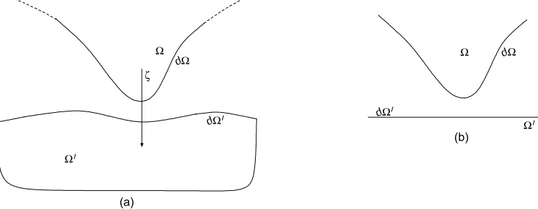
Figure 3: Geometry of the AFM tip and sample with the assumption of (a) general surfaces, and (b) a locally flat sample
To construct macroscopic relations quantifying the force between the cantilever tip and sample, we consider first the general case in which the tip and sample are arbitrary bodies Ω and Ω0 having densities ρ and ρ0.
so that summation can be replaced by integration, and (iii) constant material properties. For these assumptions, the force exerted by the particule located in x0 on this inx is given by
FvdW =ρρ0 Z
Ω Z
Ω0
f(x0−x) dxdx0 (35)
where f =−∇W.
The determination ofF for arbitrary geometries and potentialW necessitates approximation of integrals over six dimensions which is typically prohibitive. To simplify the formulation, we follow the approach of [26, 27] and reformulate the relation in terms of surface integrals. We consider the vector field
G= −Cζ
3||ζ||6. (36)
It follows that
divG=−W (37)
and hence the divergence theorem can be invoked to formulate the macroscopic force as
FvdW =ρρ0 Z
∂Ω Z
∂Ω0
(G.n0)n ds0ds (38)
where nandn0 respectively denote normals to the tip and sample. For the vector field relation (36), the force is
FvdW =− A 3π2
Z
∂Ω Z
∂Ω0
ζ.n0 ||ζ||6n ds
0ds (39)
where the Hamaker constant is
A=π2Cρρ0. (40)
The flat sample case: For various applications, it is reasonable to approximate the sample by a locally flat surface (n0constant) while retaining the general representation for the cantilever tip, see Figure 3 (b). For example, this assumption is reasonable when identifying the tip shape using a known sample with minimal curvature or for regimes in which the separation distance is large compared with perturbations in the sample. From the approximation
Z
∂Ω0
ζ.n0
||ζ||6n ds≈
Z
R2
ζ.n0
||ζ||6 dx 0 1dx02 =
Z
R2
ζ.n0
||ζ||6 dζ1dζ2 =
π
2(ζ.n0)3.
the attractive force is
FvdW = A 6π
Z
∂Ω
n
(ζ.n0)3 ds. (41)
R
d
θ
γ
x3
Figure 4: Geometry of the AFM tip
Flat sample and parameterized tip: Finally, we consider the case in which the sample
surface is assumed locally flat and a simple geometric parameterization is assumed for the cantilever tip. Specifically, we follow the approach of Argento and French [26] and assume that the cantilever can be parameterized as having a spherical tip of radiusR, and a conical section as depicted in Figure 3 with a distancedfrom the sample. This geometry is motivated by scanning electron microscopy (SEM) images of various AFM tips and provides sufficient flexibility for a number of applications while limiting to commonly employed models for spherical probes.
This assumption allows cylindrical symmetry to be invoked to yield analytic force relations, and relaxation of this assumption would necessitate the approximation of nonsymmetric con-tributions which yield higher-order force effects.
As detailed in [26], the attractive force due to van der Waals interactions can in this case be expressed as
FvdW(d) = AR
2[1
−sinγ][Rsinγ−dsinγ−R−d] 6d2[R+d−Rsinγ]2 −
Atanγ[dsinγ+Rsinγ+Rcos(2γ)] 6 cosγ[d+R−Rsinγ]2
(42)
where A is the Hamaker constant specified in (40) andγ is the cone angle shown in Figure 3. The repulsive forces are due to the overlap of electron clouds. These are quantum mechan-ical in nature and very short range compared with the attractive forces. Phenomenologmechan-ical arguments yield microscopic potential relations of the form
Wrep(ζ) = B
||ζ||12 (43)
where B is a constant which depends on electronic and material properties of the sample and tip. Arguments analogous to those for the attractive forces yield short-range force relations analogous to (39), (??), or (42).
6
Examples
6.1
A Single AFM
The two-dimensional domainωP is a rectangleωP = (0, `0C)×(0, LC)with`0C << LC.The plate
is made up of an homogeneous isotropic material, is clamped on the sidex1 = 0and is left free otherwhere. The elastic part is ωE = (0, `0C)×(0, LE) and the rigid part is its complementary
set ωR = (0, `0C)×(LE, LC). The coordinates of the tip arextip = (xtip1 , x
tip
2 , x
tip
3 ). The shape of the sample to be analyzed is parameterized by a function φ(x1, x2). The force applied on the tip is modelled as a concentrated force
f1 =f2 = 0 andf3(x) =F(d)δxtip(x)
where d=utip
−φtipwithφtip =φ(xtip1 , xtip2 )andutip =u(xtip). Let us denote byxG the gravity
center of ΩR and assume that xtip−xG is parallel to the direction of x3. If the dependency of
uP3 with respect to x1 is neglected, then the distance d between the tip and the sample is the unique solution of the nonlinear algebraic equation
kP(xtip2 )(d+φtip)−F(d) = 0 (44) and when d is knownuP3 is computed by
uP3(x2) = F(d)/kP(x2) for x2 ∈[0, LC]
where
kP(x2) =
6mP
x2
2(3HP|ωR|/|ΩR|−x2)
in[0, LE]
= 6|ΩR|m
P
LE(−3LEHP|ωR|+ 2L2E|ΩR|+ 6x2HP|ωR|−3x2LE|ΩR|)
in (LE, LC],
and
mP = 8µa
3(λ+µ)`0
C
3(λ+ 2µ) , (45)
hP =|ωR|−1|ΩR|, HP =|ωR|−1
Z
ωR
(a+h(x))x2 dx.
The proof is straightforward and we mention only the main steps. From Section 7.4,
fP(x) = a+h(x)
|ΩR|
F(d) in ωR, fP = 0 inωE, gP = 0 inωP,
thus
ξP =
Z
ωR
a+h(x)
|ΩR|
dx F =F andΞP2 =
HP
|ωR|
|ΩR|
F.
The displacement uP
3 is solution of the boundary value problem
d4uP3
dx4 2
(x2) = 0 for x2 ∈(0, LE), uP3(0) =
duP3
dx2
(0) = 0
(46)
−mPd
3uP
3
dx3 2
(LE) = ξP and mP(
d2uP
3
dx2 2
−d
3uP
3
dx3 2
where mP =`0CRP2222. In the rigid part
uP3(x2) =bP +B2Px2
with
bP =uP3(LE)−
duP
3
dx2
(LE)LE andB2P =
duP
3
dx2
(LE).
In particular,
utip =bP +B2Px
tip
2 . The equations (46) yield uP
3(x2) =a0+a1x2+a2x22+a3x32 in the elastic part with
a0 =a1 = 0, 2mPa2 =ΞP2 and −6mPa3 =ξP (47)
from which the equation uP
3(x2) = F(d)/kP(x2) follows. The equation of d follows by taking
x2 =xtip2 and using the relation uP3(x
tip
2 ) =d+φ
tip.
6.2
An AFM Array
The whole system is still comprised of a homogeneous isotropic material. The subdomains YB
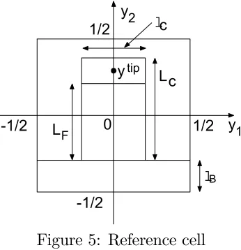
andYCare two rectangles described respectively in the coordinates(OB, y1B, y2B)and(OC, yC1, y2C) by
YB = (0,1)×(0, `B) andYC = (0, `0C)×(0, LC)
where OC = (− `0
C
2 , `B− 1
2), OB = (− 1 2,−
1 2), y
B = y
−OB and yC =y−OC, see Figure 5 for
the description of the cell and Figure 4 for the changes of coordinates.The flexible part YF of
YC is (0, `0C)×(0, LF) in(OC, yC).
-1/2
1/2 -1/2
1/2
0
lB lc
y2
y1
Lc
LF
tip
y
Figure 5: Reference cell
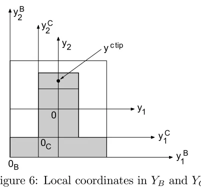
We assume thatγM1 =∅ soγM0 ={0,1} ×(0,1). The tip coordinates are denoted by ytip in
(O, y1, y2), byyCtip in (OC, y1C, yC2) and byx
tip i = (x
tip i1 , x
tip i2 , x
tip
C
0 y
y
y2
2B 2
0C
0B
y1
y1C
y
1B
yc tip
Figure 6: Local coordinates inYB andYC
The force applied to the cantilever is assumed to be concentrated on each tip, so that
f1 =f2 = 0andf3(x) =
X
i
F(u3(xtipi )−φ(x tip
1i , x tip
2i ))δxtipi (x) inΩ.
The corresponding volumic force can be computed by using the results of Section 7.4. We assume that it satisfies the assumptions done for the derivation of the two-scale model. Then for d(x) = uM(x) +uC(x, yCtip)
−φ(x), the model is stated as follows. The couple (d, uM) is
solution of
RM11∂x41x1x1x1uM(x) =F(d(x))/ε for all x∈ω (48)
uM(0, x2) =uM(1, x2) =∂x1u
M(0, x
2) =∂x1u
M(1, x
2) = 0 for allx2 ∈(0, L2) and
kC(y2Ctip)(d+φ−u
M
)(x)−F(d(x))/ε= 0 for allx∈ω. (49)
Once d is known,uC is computed by
kC(y2C)uC(x, y2) =F(d(x))/ε for all (x, y2C)∈ω×(0, LC)
where
kC(y2) =
6mC
y2
2(3HC|YR|/|VR|−y2)
in[0, LF]
= 6|VR|m
C
LF(−3LFHC|YR|+ 2L2F|VR|+ 6y2HC|YR|−3y2LF|VR|)
in (LF, LC],
HC =|YR|−1
Z
YR
(aC +h0(y))y2 dy, h0(y) = h(xi +εy)/ε,
RM11 =
4µa3B`Bε4
3(λ+ 2µ)(2λ+ 2µ−
λ2
2(λ+µ)), m
C = 8µa
3
C(λ+µ)`0C
3(λ+ 2µ) .
Moreover, LB(∇∇TuM) = − 2λ 4(λ+µ)
µ
0 0 0 1
¶
and aC for the thickness of the base and of the cantilever divided by ε and VR ⊂ R3 the
three-dimensional dilatation of any of the tips in ΩR.
Let us sketch the derivation. From Section 7.4, the surface force in the thin plate model is
fP(x) =X
i
aC +h0((x−xi)/ε)
|VR|
F(uP(xtipi )−φ(x tip
i ))χYi(x)
where xtipi = (xtipi1 , xtipi2) anduP stands for the approximation of u
3.Its two-scale transform is
b
fP(x, y) = aC +h
0(y) |VR|
F(buP(x, ytip)−bφ(x, ytip))/ε2
then
f0(x, y) = aC+h
0(y) |VR|
F(uM(x) +uC(x, ytip)−φ(x))/ε2.
From that expression, one may derive the solutions of the three problems PB,
PM and
PC.
Problem PB : The solutionwB of PB is
wB(yB) =− λν 4(λ+µ)(y
B
1 )2.
This is verified by showing that such wB satisfies the variational formulation. Thus
MB = 8µK 3(λ+ 2µ)
µ
λ 0
0 2(λ+ 2µ)
¶
with K =− λν 4(λ+µ)
and
Z
YB
MB∇y∇Tyv dy=
16µ(λ+µ)K
3(λ+ 2µ)
Z
YB
∂y21y1v dy
because RY
B∂
2
y2y2v dy = 0 due to the periodicity of∂y1v onγper.By another way,
FB = 4µ 3 (
ν λ+ 2µ
µ
2(λ+µ) 0
0 λ ¶ + µ 0 α α 0 ¶ ) then Z YB
FB∇y∇Tyv dy=
4µλν
3(λ+ 2µ)
Z
YB
∂y22y2v dy
because RY
B∂
2
y1y1v dy = R
YB∂
2
y1y2v dy = 0 due to the periodicity of v and ∂y1v. Finally the
variational formulation
Z
YB
MB∇y∇Tyv dy=−
Z
YB
FB∇y∇Tyv dy
is fulfilled.
Problem PM : It is straightforward to verify that
LBξζγδ =−
2λ
4(λ+µ)δξ2δζ2δγ1δρ1
e
RMαβγρ= 4µ`Ba
3
Bε3
3 (
λ
λ+ 2µδαβδγρ+δαγδβρ−
λ
2(λ+µ)(
λ
It then follows that
RM =
Re
M
1111 0
0 16`Bµ 3
with ReM1111 = 4`Bµa
3
Bε3
3(λ+ 2µ)(2λ+ 2µ−
λ2
2(λ+µ)).
The macroscopic forces are fM
1 (x) = F(d(x))/ε2 andf2M = 0. Then multiplying the equation of uM by ε and introducingRM
11 =εRe1111M , one find that uM is solution of the boundary value problem (48) and θ is solution of
∂x21x1θ(x) = 0 for x∈ω, θ(0, x2) =θ(1, x2) = 0 for allx1 ∈(0,1)
thus θ = 0.
Problem PC : The calculations are exactly the same as those for the simple plate model
in Section 6.1 excepted that x, LE, uP3, ξ
P
, ΞP
2, bP, BP2, ΩR, ωR and HP are replaced by yC,
LF, uC, ξC, ΞC2, bC, B2C, VR, YR andHC. Neglecting the variations of uC with respect to y1 it comes that uC depends ofx and y
2 only and is solution of the boundary value problem
∂4uC
∂y4 2
= 0 for y2C ∈(0, LF), uC =
∂uC
∂y2
= 0for y2C = 0 (50)
−`CRP2222ε− 4∂3uC
∂y3 2
= ξC and`CRP2222ε− 4
(∂
2uC
∂y2 2
− ∂
3uC
∂y3 2
y2C) =Ξ
C
2 for y
C
2 =LF
and
ξC(x) = F(d(x))/ε2,
ΞC2(x) = |VR|−1
Z
YR
(aC+h0(y))y2 dy F(d(x))/ε2 = |
YR|HC
|VR|
F(d(x))/ε2.
By introducing mC = `
CRP2222ε−3 The expression of uC follows. Finally by using the relation
uC(., y2) =d−uM +φ for y2C =y
Ctip
2 the equation (49) follows.
6.3
Numerical Simulation of the AFM Array
For numerical computation the algebraic equation (49) is replaced by
(d+φ−uM)(R+d−Rsin(γ))2d2−(kC)−1G(d) = 0 (51) where G(d) = ε−1F(d)(R +d−Rsin(γ))2d2. F(d) = FvdW(d) +Frep(d) where the van der WaalsFvdW is defined in (42) from the potential (34) and the repulsive forceFrep is build from
(43) on the same way. In order to avoid numerical errors due to the presence of large and small values in the system, we use the normalized functions and variables
x∗1 =x/L1, x∗2 =x2/L2, uM∗(x∗) =uM(x)/φscal, d∗(x∗) = d(x)/φscal,
φ∗(x∗) =φ(x)/φscal, F∗(d∗) =L41F(d∗φscal)/(RM11φscal), G∗(d∗) = G(d∗φscal)/φ3scal, R∗ =R/φscal, k∗ =kC(ytip2 )φ2scal
so that (48) and (51) are replaced by
∂x4∗
1u
M∗ =F∗(d∗)andE(d∗, uM∗) = 0 in (0,1)2
uM∗(x∗) = ∂x1u
with E(d∗, uM∗) = (d∗+φ∗−uM∗)(R∗+d∗−R∗sin(γ))2(d∗)2−k∗−1G∗(d∗).The displacement
uM∗ is decomposed on the basis of eigenfunctionsψ
m(x∗1) :
uM∗(x∗) =
Nu
X
n=1
Un(x∗2)ψn(x∗1)
where
∂x4∗
1ψn(x ∗
1) =λnψn(x∗1)for all x∗1 ∈ (0,1)and ψn(x∗1) =∂x1ψn(x∗1) = 0 for x∗1 ∈{0,1}, then
Un(x∗1) =
Z 1
0
F∗(d∗(x∗))ψn(x∗1) dx∗1/λn. (52)
The functions φ∗ andd∗ are decomposed on the normalized orthogonal Chebychev polynomials
Pn on(0,1) :
φ∗(x∗1) =
Nφ X
n=1
Φn(x∗2)Pn−1(x∗1) andd∗(x∗1) =
Nd
X
n=1
Dn(x∗2)Pn−1(x∗1).
Thus the second equation is replaced by
E(D,Φ, U) = 0
where
E(D,Φ, U) =E(
Nd
X
n=1
Dn(x∗2)Pn−1(x∗1),
Nφ X
n=1
Φn(x∗2)Pn−1(x∗1),
Nu
X
n=1
Un(x∗2)ψn(x∗1)).
The discretized system is solved by replacing Un by its expression (52) and then by searching
the minimum of R01E2(D,Φ, U) dx∗
1 with respect to D. The minimum search is conducted by combining a minimizing method relatively to D and a length line continuation with respect to the number of cells. The algorithm is initialized with a small number of cells whereuM∗ is close
to zero. Then the number of cells is increased incrementally.
We have conducted computations with a square cell having a length ofε= 50µm.The other parameters areLC = 0.5, `0C = 1/16, aC = 1/40, y2Ctip = 7/16, LF = 3/8, `B = 1/4, aB = 1/10,
A = 1.25e −19J, γ = π/6, R = 10−7m, λ = 6.1e11, µ = 5.2e11, φ
scal = 10−9 and finally
the shape of the tip is chosen so that (kC(ytip
2 ))−1 = 3e−8. The number of cantilevers or equivalently the length of the array is a parameter chosen in each experiment. In the following we refer to three choices of φ∗ corresponding to three values of Nφ:
Nφ = 1 :φ∗(x∗1) =
φ0∗+φ1∗
2 ,
Nφ = 2 :φ∗(x∗1) = φ
0∗ + (φ1∗
−φ0∗)x∗1 , Nφ = 3 :φ∗(x∗1) = φ
0∗ + 4φ1∗x∗
Figure 7: Distributions of uM∗, uM∗ +uC∗ and ofφ∗ as functions ofx∗
1 for 10, 16 cantilevers
Figure 7 represents the functionsuM∗, uM∗+uC∗ at the tip locations and ofφ∗ ofx∗
1 ∈(0,1) in the case of a flat sample,Nφ = 1,for two arrays having 10 and 16 cantilevers in the direction
x1. It is not surprising to observe that when the base length increases it deforms on a non negligible way in comparison with the total displacement of the tip.
Figure 8: max
x∗
uM∗
uM∗+uC∗ with respect to the number of cells
Figure 8 illsustrates how the maximum value over x∗
1 of the ratio
uM∗
uM∗+uC∗ taken at the
tips varies as a function of the number of cells for Nφ = 1. Evidently this ratio tends to zero
for a small number of cells but it also increases dramatically with the number of cells which means that in this case the tip displacement is more governed by the base displacement than by the the cantilever deflection.
Nφ\Nd 1 3 5 7 9
1 2.2 2.8 4.3 5.7 7.4
2 1.0 2.8 3.7 3.8 3.9
3 0.7 2.7 3.4 4.0 4.7
Nφ\Nd 1 3 5 7 9
1 1.5 2.1 3.6 4.9 5.8
2 1.0 2.1 3.6 4.6 4.7
3 0.6 2.5 3.4 4.0 4.1
Table 1: Err for 10 cells and 14 cells depending onNφ andNd
The quality of the approximation ofd∗by using the Chebychev polynomials is also of interest. In table 1, we report the order of magnitude of the error on d∗
Err =−log10err where err 2
=
R1
0(d∗Nd(x ∗
1)−d∗(x∗1))2 dx∗1
R1
7
Appendix
In this appendix, we report some mathematical definitions and properties. The concept of weak and strong approximation are defined in Section 7.1. Then in Section 7.2 the two-scale transform of a function is defined and its elementary properties are stated. Weak approximations of first order and second order derivatives two-scale derivatives are derived in Section 7.3. In Section 7.4 we provide the expression of a volumic force which action is equivalent to a concentrated force when it is applied in the rigid part. This result is used in the examples of Sections 6.1 and 6.2. Finally a fundamental inequality used for the derivation of the two-scale model is stated and proved in Section 7.5.
7.1
Weak and strong Approximation
Consider an open set A ∈ Rn, wε
∈ L2(A), a function depending on the parameter ε and a function w0 ∈ L2(A) independent of ε. We say that wε = w0 +O(ε) weakly in L2(A) if
R
A(w
ε
−v0)v dx=O(ε)for all v
∈L2(A) and we say that the same equality holds strongly in
L2(A) if RA(wε−w0)2 dx=O(ε).
For example the oscillating function sin(xε) can be approximated by zero in the weak sense but cannot be approximated by a function independent of ε in the strong sense.
7.2
Properties of the Two-Scale Transform
We state here some elementary properties of the two-scale transform. The proofs are elementary and are not detailed here. Some may be found in M. Lenczner and G. Senouci [11].
Forv, w∈L1(ω),
\
v+w=bv+w,b vwc =bvwb and
Z
ω
v(x)dx=
Z
ω×Y b
v(x, y)dydx
For v∈L2(ω),
||v||ω =||bv||ω×Y
and if ∇v∈L2(ω) then
c
∇v=ε−1∇ybv.
For any εY−periodic part ωx of ω (like ωP) and Yx its corresponding reference cell in Y, it
follows that
d
χωx =χω×Yx.
It is convenient to note that the two scale transform is a linear operator T defined fromL2(ω) to L2(ω
×Y) byT u=bu. Its adjoint T∗ is defined by Z
ω
u(x)(T∗v)(x) dx=
Z
ω×Y
(T u)(x, y)v(x, y) dxdy (53)
for allu ∈L2(ω) andv
∈L2(ω
×Y). A direct computation shows that
T∗v(x) =X
i
ε−d Z
Yε
i
v(z,x−xi
ε )dz χYiε(x) =
X
i
ε−d Z
Yε
i
v(z,x
where the function v is defined on ω× 1εω byv(z, y) =Piv(z, y− xi ε)χYε
i(z). Apparently v is
not continous on ω; however if v is extended as an Y−periodic function on Rd then v can be
rewritten as
v(z, y) = v(z, y−1
2) for(z, y)∈ω× 1
εω (54)
and has evidently the same periodicity with respect to its second variable and the same diff er-entiability with respect to both variables asv. It is useful to make the remark that ifvis k+ 1
times continuously differentiable with respect to its first variable thenT∗vcan be approximated
up to the order k with an expansion inε,
T∗v=
k
X
j=0
fkεk+εkO(ε) (55)
whose coefficients are some functions ofv(x,xε)and their derivatives. It turns out that the first coefficients are
f1 = v(x,
x
ε),
f2 = −X(x).∇xv(x,
x
ε)
f3 =
1
2X(x)∇x∇
T xv(x,
x
ε)X(x) +
1
12∆xv(x,
x
ε)
where X = T∗(y). The calculation of these coefficients is straightforward. One starts by
applying the Taylor formula to v at(x, y) with respect to its first variable: v(z, y) =v(x, y) +
∇xv(x, y)(z−x) + 12(z−x)T∇x∇xTv(x, y)(z−x) +ε2O(ε) for x, z∈Yiε. Then one substitutes
it in the expression of T∗v. The calculations of the integrals are carried out by using the
decompositionz−x= (z−xε
i)+(xεi−x)and the identities
R
Yε
i (z−x ε
i)dz = 0and
P
iχYε
i(x) = 1.
Conversely one deduces an approximation of v(x,xε):
v(x,x
ε) =T
∗(v+ε(y.∇
x)v+
ε2
2(y.∇x)
2v
− ε
2
24∆xv)(x) +ε
2O(ε), (56)
which is derived by applying the second order approximation (55) and replacing ∇x∇Txv, ∆xv
with their zero order approximation and ∇x∇Tyv with its first order approximation.
The two-scale transform is a linear operator that is well defined on functions. Its definition can also be extended to some generalized functions or distributions: vbeing such a generalized function T v is defined formally by duality
Z
ωh
T v, wiy dx=hv, T∗wix
for all w belonging to a class of regular functions defined on ω ×Y. From this definition the two-scale transform of
v(x) =g(x)X
i
δxi+εy0(x)
T v is found to be
where y0 ∈Y, δξ is the Dirac distribution in ξ and g is any regular function. Indeed,
hv, T∗wix =
*
g(x)X
i
δxi+εy0(x),
X
j
ε−d Z
Yε
j
w(z,x
ε)dz χYjε(x)
+
x
= X
i
g(xi+εy0)ε−d
Z
Yε
i
w(z, y0)dz =ε−dX
i
Z
Yε
i
T g(z, y0)w(z, y0)dz
= ε−d Z
ω
T g(z, y0)w(z, y0)dz =ε−d Z
ω
T g(z, y)δy0(y), w(z, y0) ®
y dz.
This means that T v(z, y) =ε−dT g(z, y)δy0(y).
7.3
Approximations of the Two-Scale Transform of the Derivatives
The following results are stated in the general case where d is any positive integer, ω =
Πd
i=1(0, Li) and Y = (−21,12)d with Li some non negative numbers. The definitions of the
cells Yiε and of the two-scale transform (15) still hold.
Notation: Consider a εY−periodic set ω1 ⊂ ω with cells Y1εi and the associated unit cell
Y1 = 1ε(Yiε−xεi) ⊂ Y. The intersection between the boundaries of Y1 and of Y is denoted by
γper, it corresponds to the location where the cells Y1εi are connected. We take into account
cases where the cells Yε
1i are connected to their neighbors in some directions but not in the
others. Then the gradient splits in two parts ∇ = ∇C +∇N C where ∇C and ∇N C contain respectively the partial derivatives in the connectivity directions and in the directions without connectivity. In the same way, the components y and the unit outwards normal vectors n to a boundary (∂ω or ∂Y1) split as y= yC +yN C andn=nC +nN C. The extremal cases where the cells Y1εi are connected in all directions (∇
C
= ∇, nC = n and yC = y) or in none of them (∇C =nC =yC = 0) are encompassed by these notations. The part of the boundary∂ω
where the unit outward normal vector nC
x 6= 0 is divided into γM0 where boundary conditions are applied and γM1 .
First order derivatives: Letube a function defined onω1,depending on the parameterε, vanishing on γM
0 ∩∂ω1 and such that its norms ||u||ω1 and||∇u||ω1 areO(1) with respect to ε.
From the norm conservation through the two-scale transform, we already know that ||bu||ω×Y1
and ||∇cu||ω×Y1 are also O(1). If, in any manner, it is known that ubadmits an expansion with
respect to ε on the form bu = u0 +εeu1 +εO(ε), at least in the weak sense, with u0 and ue1 independent of ε, then u0 = 0 onγ
0,∇yu0 = 0onω×Y1,
c
∇u=∇Cxu0+∇yu1+O(ε) onω×Y1 (58)
in the weak sense,u1 =eu1
−yC.
∇Cxu0,u1 isY−periodic onγper, u0 ∈L2(ω),∇ C
xu0(x)∈L2(ω)d,
u1
∈L2(ω
×Y1) and∇yu1 ∈L2(ω×Y1)d.
Second order derivatives: In addition, we assume that||∇∇Tu||ω1 is O(1), that ∇u= 0
on γM
0 ∩∂ω1 and that bu=u0+εue1+εue2+ε2O(ε), at least in the weak sense. It then follows that ||∇∇\Tu||ω×Y1 isO(1),∇xu
0 = 0on γ
0, ∇y∇Tyu1 = 0, ∇ C
yu1 = 0,
c
∇u = ∇Cxu0+θN C +O(ε) (59)
and∇∇\Tu = ∇Cx(∇Cx)Tu0+∇Cx(θ N C
)T + (∇Cx(θ N C
on ω×Y1 in the weak sense, u2 =ue2−yC.∇Cxue1+ (yC.∇ C
x)2u0, u2 and∇yu2 are Y−periodic
on γper, θN C = ∇N Cy u1 which is independent of y,
∇Cx(∇ C
x)Tu0 ∈ L2(ω)d×d and ∇ C x∇yu1,
∇∇Tu2
∈L2(ω
×Y1)d×d.
Strong variations, first order derivatives: In the case where the variations of u are
sufficiently large that ||∇u||ω1 is not of order O(1)but||ε∇u||ω1 isO(1) andbu=u
0+O(ε), at least in the weak sense, then ∇yu0 ∈L2(ω×Y1) and
ε∇cu(x, y) =∇yu0 +O(ε) (60)
in the weak sense.
Strong variations, second order derivatives: If in addition ||ε2∇∇Tu||ω1 is O(1) then
∇y∇Tyu0 ∈L2(ω×Y1) and
ε2∇∇\Tu(x, y) =∇∇Tu0+O(ε). (61)
Here we sketch the proof of these approximations by indicating the calculation steps without going into precise mathematical justifications.
Proof for the first order derivative: The proof is decomposed into four steps. (i) If ||∇u||ω1 is O(1) then ∇yu
0 = 0. This comes from the properties of the