Investigation of Remote Sensing Derived Surface Temperature and Normalized Difference Vegetation Index and Implications for Land Cover Classification
by
Francis George Davis
A Project submitted to the Graduate Faculty of North Carolina State University
in partial fulfillment of the requirements for the degree of
Master of Natural Resources Assessment and Analysis Option
Raleigh, North Carolina 2013
APPROVED BY:
ABSTRACT
Davis, Francis George. Investigation of Remote Sensing Derived Surface Temperature and Normalized Difference Vegetation Index and Implications for Land Cover Classification. (Under the direction of Dr. Gary Blank, Dr. Ryan Emanuel, and Dr. Heater Cheshire). This research investigates the relationship between surface temperature (Ts) and the
Normalized Difference Vegetation Index (NDVI) as a proxy for leafy green biomass across a landscape in Southern Kenya. The two parameters, derived from Landsat 7 data are
compared between and across land cover types in 2000 and 2005 to see how the relationship varies among different ecosystems. This work serves to investigate how plant community composition affects energy transformation. It is well documented that NDVI and Ts are
inversely proportional and correlated. However, based on the assumption that different ecosystems process solar energy differently, it is hypothesized that the strength and direction of this relationship will vary significantly between different land cover types. Due to this variable relationship Ts is a useful ancillary data source for land cover classification,
especially in the early stages of a hierarchical classification protocol. Ts is demonstrated to be
more robust and resilient to inter-annual climatic variation compare to NDVI. Furthermore, Tukey’s Honest Significant Difference based on mean rank found that the number of land classes that were significantly different increased when both Ts and NDVI were used rather
BIOGRAPHY
TABLE OF CONTENTS
I. Problem Statement ... 1
II. Introduction ... 2
III. Background ... 4
IV. Method ... 11
a. Study Area ... 11
b. Image conversion and calibration ... 17
c. Vegetation Indices ... 18
d. Temperature Calculation ... 18
e. Analysis ... 19
V. Results ... 23
VI. Discussion ... 46
VII. Conclusion ... 51
LIST OF TABLES
Table 1. Landcover Type and Subtypes Descriptions from Africover (FAO, 1999)... 23
Table 2. Tukey Honest Significant Difference Test (α=0.01) 2000 ... 43
Table 3. Tukey Honest Significant Difference Test (α=0.01) 2005 ... 43
Table 4. Tukey Honest Significant Difference Test (α=0.01) ... 44
Table 5. TNDVI Relative Rank ... 44
LIST OF FIGURES
Figure 1. Results from Discriminate Analysis (Southworth 2010) ... 3
Figure 2. Energy balance components using Thermal Infrared Multispectral Scanner (Luvall and Holbo, 1991 in Schneider and Kay, 1994)... 7
Figure 3. Maximum Spectral Radiance (Dash, 2002) ... 8
Figure 4. Sample Spectral Signature from USGS Spectroscopy Library (Clark et al, 2007) ... 10
Figure 5. Digital Elevation of Study Area with 500 Meter Elevation Contours ... 13
Figure 6. Africover Land Cover Classification -Kenya Aggregate Landcover - 1:100,000 scale ... 16
Figure 7. Scatterplot Mean TNDVI vs. Ts, 2000 ... 27
Figure 8. Figure 7. Scatterplot Mean TNDVI vs. Ts, 2005 ... 28
Figure 9. Ts for Landsat 7 Scene 168,61 February 2000 ... 31
Figure 10. Ts for Landsat 7 Scene 168,61 February 2005 ... 32
Figure 11. Box and Whisker Charts Ts Statistics, 2000 and 2005 ... 33
Figure 13. Box and Whisker Charts for TNDVI Statistics, 2000 and 2005 ... 33
Figure 12. TNDVI for Landsat 7 Scene 168,61 February 2000 ... 35
Figure 13. TNDVI Landsat 7 Scene 168,61 February 2005... 36
Figure 14. Box and Whisker Charts TNDVI Statistics, 2000 and 2005 ... 37
Figure 15. Spearman’s Rank Correlation Coefficient, 2000 and 2005 ... 39
Figure 16. Comparing the Change in Spearman’s Coefficient ... 40
Figure 18. Landsat 7, Band 5, 2000 ... 47
I.
Problem Statement
The application of energy transformation research to ecology is a fertile and
rewarding, but vexing, avenue of research. The laws that govern the behavior of matter and energy are integral for determining what a natural system can and cannot due, and represent basic constraints to any ecological system. These constraints are powerful tools that make prediction of system behavior possible. This was demonstrated nearly a hundred years ago when Transeau (1926) calculated the energy budget of an acre of corn in central Illinois. This is possible due to the first law of thermodynamics, which is concerned with the quantity of energy and matter. It is a powerful constraint: because they can never be destroyed or
created, the energy and matter which enters a system must either remain in the system or exit the system in the same quantity, although possibly in different form.
Complex natural ecosystems behave differently and process energy differently than a single organism or a single species of organism. This complex behavior complicates the investigation of the energy budget of ecological systems. An assessment of the relationship between biomass and the transformation of incoming solar energy into sensible heat for various land cover types within one local area with minimum climate and geomorphologic variation as outlined in the above introduction will demonstrate how this relationship varies between land cover types.
on the hypothesis that energy transformation efficiency depends on the condition and community composition of the ecosystem being investigated.
This investigation will also have practical utility through the potential application of the results to land degradation and classification work for local and regional land managers. Land degradation is defined broadly as a reduction in the capacity of land to provide
ecosystem services. This is useful for developing policy, because it allows the inclusion of many different processes and forms that constitute degradation. However, for researchers and scientists, specific and objective indicators of degradation need to be developed that can be employed cheaply, quickly, and effectively. Further research into the relative efficiency of energy transformation in ecosystems is important to objectively assess ecosystem states and specifically, land degradation.
II.
Introduction
production of different land cover types the relative efficiency of different plant communities in processing absorbed solar energy could be determined. This method can be utilized on a larger scale using widely available satellite remote sensing data.
Southworth (2004) integrated Landsat band 6 (10.4 to 12.5 micrometer) derived thermal data into land cover classification and found land cover classes were strongly related to surface temperature (figure 1). Band 6 thermal data outperformed many other bands in its ability to discriminate between land classes, despite its lower resolution. Previous studies have used satellite data to obtain the temperature of the Earth’s surface (Qin et. al. 2001,
Goode and Palle 2007, Zhang et. al. 2007).
Figure 1. Results from Discriminate Analysis (Southworth 2010)
Using remote sensing data from the Landsat 7 Enhanced Thematic Mapper (ETM+) satellite to calculate surface temperature (Ts) and the normalized difference vegetation index (NDVI)
this research investigates how different ecosystems process energy. Assuming that climatic conditions are similar at the local scale of one Landsat 7 scene, if there is a different strength of correlation between these two parameters from one land cover type to another, then surface temperature depends not only on the amount of green biomass (NDVI), but also on type and community structure of the land cover type. This will demonstrate that the
relationship between the variables Ts and TNDVI changes based on land cover type.
III.
Background
When solar radiation enters the earth’s atmosphere, a portion of it is reflected and scattered. The portion of radiation that reaches the earth’s surface is either reflected back into the atmosphere as long-wave radiation or absorbed into the surface. Both reflected radiation and absorbed radiation can be degraded into molecular motion in the form of either sensible or latent heat.
1.
= net flux of solar radiation (incoming) = net flux long wave radiation (outgoing)
= net radiation flux absorbed at surface (degraded from radiation into molecular motion)
2.
= sensible heat flux (heat transfer with no phase change and with temperature change) = latent heat flux (heat transfer with phase change and no temperature change)
Solar radiation is dissipated through evaporation as latent heat according to the latent heat of vaporization, or the energy required for vaporizing one unit mass of water at standard pressure ). Similarly, solar radiation is dissipated as sensible heat by the specific heat capacity, or the energy required for raising one unit mass of a substance by one degree kelvin ). The partitioning of net flux radiation absorbed at the surface into latent and sensible heat is determined by density, pressure, temperature, humidity, and solar radiation. These parameters can be estimated using the eddy covariance method described above. Vegetation characteristics also mediate this relationship due to the release of water from plant stomata as transpiration. This is more difficult to estimate and is usually approximated based on empirical data. Latent heat flux from biotic and abiotic sources is known as evapotranspiration, and can be modeled according to the Penman-Monteith equation.
3.
( (
))
ET= Water volume evapotranspired (m3 s-1 m-2)
Δ= Rate of change of saturatuin specific humidity with air temperature (Pα K-1
) Rn = Net Radiation (W m-2)
Ρa= Dry air density (Kg m-3)
Cp= Specific heat capacity of air (J kg-1 K-1)
VPD = Vapor pressure deficit (Pa) ga= atmospheric conductance (m s-1)
gs= Stomatal conductance (m s-1)
ϒ= Psychrometric constant (≈ 66 Pa K-1
Solar radiation that is absorbed by plant matter containing chlorophyll is used to catalyze the chemical reaction photosynthesis; the conversion of carbon dioxide and water into glucose and atmospheric oxygen using the energy of sunlight.
4. →
Photosynthesis is a major source of chemical energy in terrestrial ecosystems and is the basis of primary productivity. Due to conservation of mass as dictated by the first law of thermodynamics, rates of photosynthesis can be calculated from CO2, water, and sunlight
input. The fuel produced by primary production is utilized by other organisms on higher trophic levels and forms the basis of energy inputs into ecosystems. It is also the basis of agriculture and the production of biomass as an economic commodity. Photosynthesis also produces heat waste that is dissipated and reradiated into the atmosphere. This heat has major climate implications in either of its forms: latent heat which is transferred from liquid to gas water through the phase change with no temperature change, or sensible heat which is transferred with to liquid or gas with no phase change and a temperature change. Steinborn and Svirezhev (2000) suggested that the relative increase in disorder by one ecosystem compared to another due to the production of waste sensible heat be a quantitative indicator of ecosystem condition, but so far disorder cannot be measured directly.
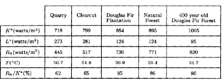
Schneider and Kay (1994) reviewed research conducted by Luvall and Holbo (1989)
reradiated energy (figure 2). This research also demonstrates the utility of classifying and assessing ecosystems based on their relative production of sensible heat. Although in this methodology, and the methodology which is presented below, there is no way to measure latent heat production, it can be assumed that if incoming radiation and reflected radiation are constant across a local area, latent, and sensible heat are additive portions of the total
reradiated heat. If it is assumed that the total radiated heat is constant across a local area at a single time, then sensible heat values are comparable.
Figure 2. Energy balance components using Thermal Infrared Multispectral Scanner (Luvall and Holbo, 1991 in Schneider and Kay, 1994)
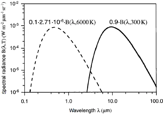
Absorbed energy is reradiated from the surface of the earth at a different wavelength
range than the reflected solar radiation (figure 3). Because of the spectral separation of
reflected and reradiated energy to different parts of the Electromagnetic (EM) spectrum,
satellite instruments which detect this energy are able to differentiate the two forms.
the surface of the earth can be estimated from the detection of reradiated heat by satellite
remote sensing instruments such as Landsat 7.
Figure 3. Maximum Spectral Radiance (Dash, 2002)
The EM radiation unequally distributed over all wavelengths of the EM spectrum, and the distribution is related to the properties of the material from which it is emitted, reflected, or refracted. Wavelength is the distance over which the wave’s shape repeats, and for EM radiation can range from 10-12 to 103 meters. The portion of EM radiation that the human eye can detect is known as visible light and ranges from 3.9 to 7 * 10-6 meters. This range is biologically important because it contains the wavelengths of EM radiation that are utilized for photosynthesis.
Radiance (rs) detected by a satellite is defined as the energy per unit time per unit
atmosphere, plus atmospheric contribution along an upward path due to scattering, plus atmospheric irradiance of that fraction of electromagnetic radiation that is reflected by the earth’s surface. Land surface temperature (LST) is more difficult to calculate than top of atmosphere (TOA) temperature due to differences in atmospheric transmissivity from
temperature and water vapor content differences, as well as local differences in emissivity of surface material. Because this study is interested in only the local area within the boundaries of one land sat scene, atmospheric effects and emissivity will be assumed to be constant.
The distribution of reflectance across a range of wavelengths is known as a spectral signature (Clark et al., 2007). The spectral signature is unique or different surface materials and represents reflectance and absorption across different wavelengths. Figure 4 depicts the spectral signature for an Oak leaf, Kaolinite and Smectite clay, water, and wetland surface. The normalized difference vegetation index is a normalized ratio of the reflected
electromagnetic radiation in detected by bands 3 (0.63-0.69 μm) and band 4 (0.76-0.90 μm) of the landsat 7 satellite instrument. These wavelengths correspond to near infrared (NIR) and Red (VIS), respectively. Photosynthetic compounds such as chlorophyll absorb light in the VIS region, but reflect light in the NIR region of the electromagnetic spectrum. NDVI value ranges from negative to positive 1, with 1 being perfect absorption of VIS, and -1 being perfect absorption of NIR. An NDVI of 0 suggests both are absorbed equally well.
In figure 4, the Oak leaf has an NDVI of approximately 0.78, clay approximately 0.08, wetland approximately 0.78, and water -0.33. This illustrates the ability of NDVI to
the inability of NVDI to differentiate different types of plant matter. Therefore, although NDVI is useful in differentiating land cover types, ancillary data is needed to support NDVI.
Figure 4. Sample Spectral Signature from USGS Spectroscopy Library (Clark et al, 2007)
is reflected and that which is absorbed and reradiated. Visible and near infrared radiation comprised of reflected solar radiation were also used for this research. The relative
proportions of these two bands are distinct for plant matter and other material. The different combinations of detected radiation in these and other wavelength ranges known as bands collectively form a spectral pattern which is distinct for different types of surface material. This research analyzes the spectral patterns of different land cover types in order to assess a relationship between these three bands that is predictably distinct.
IV.
Method
The method that follows assesses the variability of this relationship due to land cover in order to further the understanding of energy transformation by ecosystems. This is an
analysis of the relative differences in surface temperature in a local area due to differences in land cover type and vegetation density. Although the negative correlation between vegetation and surface temperature has been well established, this analysis seeks to demonstrate that this relationship can be stronger or weaker depending on the type and condition of the vegetation community.
a.
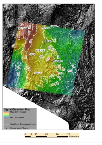
Study Area
Figure 5. Digital Elevation of Study Area with 500 Meter Elevation
The scene is path 168 and row 61 of the Landsat geosynchronous orbit. The Landsat 7 scenes are bound by the coordinates 36.41⁰, -0.503⁰ upper left; 38.099⁰, -0.747⁰ upper right; 37.753⁰, -2.375⁰ lower right; 36.06⁰, -2.131⁰ lower left (WGS 1984, UTM zone 37N) and is approximately 185 kilometers per side. These scenes were selected due to 0% cloud cover and favorable data between the dry summer and wet winter season. Furthermore, because the land cover classification is based on 1999 data, the 2000 image is the first favorable scene captured after the creation of this dataset. The 2005 image was selected in order to compare the results between time steps so that small interannual variations would not skew the results, but the land cover would not change so much to make any differences meaningless.
The bands being investigated are 3 (red), 4 (near infrared) and 6 (thermal infrared), that have wavelength ranges of 0.63-0.69 μm, 0.77-0.90 μm, and 10.4-12.5 μm, respectively. Band 3 and 4 have a spatial resolution of 30 meters squared, and Band 6 is recorded in a resolution of 120 meters, but resampled to 30 meters. Resampling is performed using a cubic convolution kernel prior to the public release of this data. This algorithm copies the 120 meter raw data onto a 30 meter resolution grid by averaging the 4*4 grids nearest to the new grid location. This method creates a smoothing and sharpening effect (Toutin, 2004).
area includes Arid Steppe (East), Temperate Dry Season (Central), and Tropical Savannah (West) (Peel et al., 2007).
Land cover data for the project area was obtained from the Africover Land Cover Classification and Mapping project-Kenya aggregate land cover-at a scale of 1:100,000. The original land cover was interpreted from Landsat imagery (Bands 4,3,2) acquired in the year 1999 (Geonetwork, 2012). The purpose of the Africover project is to produce a digital georeferenced land cover database for the whole of Africa (FAO, 1997). Based upon the international standard land cover classification system, Africover was created from Landsat TM imagery, aerial photography, and field observations. The 16 major land cover classes (figure 6) identified in the study area are: Artificial and Natural Waterbodies, Built Area, Non-built Area, Bare Area, Sparse Vegetation, Grassland, Herbaceous, Shrubland, Thicket, Woodland, Forest, Aquatic or frequently flooded Graminoid (mainly rice) Crop, Herbaceous Crop, Shrub Crop, and Tree Crop. Areas mapped with more than one of the 16 major cover types were not included in this study. Therefore, of the original 34,115 square kilometers in the scene, only 13,057 (38.3%) are single land cover types and were used in this
b.
Image conversion and calibration
Prior to public release, Landsat raw pixel values (Q) are rescaled as 8-bit digital numbers (Qcal). Conversion of Qcal to at-sensor spectral radiance (Lλ) requires knowledge of
the scaling factors used in the image pre-processing. The methodology and satellite specific scaling factors for image conversion are found in Chander, et al. (2009). Derivations of radiance, reflectance, TNDVI, and Ts are performed in ArcGIS 10 (ESRI) using the Raster
Calculator tool. First, all zero values in the band are reclassified to “No Data”, in order to avoid performing calculations on null data.
Then, digital numbers (Qdn) are converted to radiance (Lλ) for bands 3, 4, and 6 (low gain)
using the formula below.
5.
Lmax,3=234.4; Lmax,4=241.1; Lmax,6=17.04; Lmin,3=-5.0; Lmin,4=-5.1 ; Lmin,6=0;
Qmax,all=255
Next, Band 3 and 4 are converted to planetary top of atmosphere (TOA) reflectance (ρ) (Chavez, 1996). This corrects for error due to atmospheric effects that differ between sensors. Specifically, this step corrects for different values of exo-atmospheric solar irradiance and different minimum radiance values between sensors.
6. –
Lλ = band radiance (W m-2 sr-1 um-1)
= unitless planetary reflectance
Esun = mean exoatmospheric solar irradiance (Chander et. al, 2009)
Θ = solar zenith angle, or 90⁰ solar elevation (degrees), this value is found in metadata text file downloaded with each individual Landsat scene.
c.
Vegetation Indices
The normalized difference vegetation index (NDVI) is a comparison of reflectance in Band 3 and 4. This value is a measure of the difference between reflectance in the red and near infrared wavelengths. NDVI is a proxy for the amount of photosynthetic vegetation in each pixel and is based on the spectral pattern of light reflected from green vegetation (Sellers, 1985).
7.
Energy in the red wavelength detected by band 3 is absorbed by chlorophyll in green vegetation and little is reflected. However, in the near infrared wavelength detected by band 4 little energy is absorbed and a high reflectance value is recorded by the band 4 sensor. This index ranges from -1 to +1, and is a highly effective method to differentiate healthy
vegetation from dead vegetation or mineral material. NDVI is then rescaled from 0 to 100 using the following formula in order to increase the signal to noise ratio (Deering et al., 1975).
8.
d.
Temperature Calculation
black body with a spectral emissivity of 1, and includes the effect of atmospheric absorption and emission along the path between the satellite sensor and the earth’s surface at pixel x. Therefore, Ttoa is proportional, but not equal to land surface temperature. Differences in
emissivity due to land cover may increase or decrease the differences between land cover TOA values, but it is of a small magnitude (emissivity +-0.05) and is a small source of error. Furthermore, differences within land cover class due to emissivity should be very small, and no different than estimates of emissivity would produce. Satellite pre-launch constants for Landsat 7 are used in the following conversion formula (Chander et. al, 2009).
9.
⁄ (Inverted Plank’s Function)
Ttoa = Top of atmosphere/at sensor brightness temperature (K) Lλ = Radiance (W m-2 sr-1 um-1)
K1=666.09 (W m-2 sr-1 um-1) K2=1282.71 (K)
Finally, temperature is scaled from 0 to 100 using the following equation. This will allow temperature to be easily compared to TNDVI. Ts is the rescaled top of atmosphere
temperature that will be used in the remainder of this report.
10.
Ts = Rescaled top of atmosphere temperature (%)
Tmin=240 K, Tmax=322 K
e.
Analysis
generate 2000 unique random points within each land cover type for each year. The
minimum distance between random points is set at 30 meters to ensure all points fall within separate grid cells in the Landsat images. Because of the small area represented in the type “non-built area”, only 1607 random samples can be obtained. Each random point corresponds to a single pixel in the Landsat scenes.
Each randomly selected pixel in the Landsat scenes has one corresponding Ts and one
TNDVI value. The mean and standard deviation of Ts and TNDVI for each type is calculated
based on these randomly selected pixels. The means of Ts and TNDVI for each land cover
class are compared in order to assess the effect of land cover on these two related metrics. Statistical analysis is performed to test the significance of the differences in Ts and TNDI that exist between land cover types. Nonparametric methods are used because
normality of bivariate distribution cannot be established. Also, nonparametric methods do not require that variances of the treatment groups be equal. Traditional parametric statistics compare a data set to a theoretical probability distribution and make inferences about the data set based on this assumption. Nonparametric methods assign ordinal rank to the data points and draw inference based on relative ranking within the data set. While nonparametric is more susceptible certain types of sampling biases, they are a useful alternative for data with abnormal distribution or variance.
Then, correlation between TNDVI and Ts is calculated for each cover type.
correlation of +1 if all of the x values have the same ranking as the y values. A value of +1 can be interpreted as a complete explanation of the variation in y by the variable x.
Spearman’s coefficient (r2) is determined for TNDVI (x) and Ts (y) using the following
formula.
11. ∑
√∑ ∑
Spearman’s coefficient has a unique probability distribution for relatively small sample sizes. However, for samples greater than 100, critical values can be approximated by the student’s t distribution using the following equation (Zar, 1972). This value was
compared to the t table value of infinite degrees of freedom and alpha=0.01 (2.327) to determine significance of the Spearman’s correlation coefficient.
12.
√ ⁄
⁄
n = sample size
The Kruskal-Wallis test is used to compare the mean temperature and TNDVI of different land cover classes. This test is nonparametric and does not require data to have a normal bivariate distribution or homogeneity of variance. Instead, temperature and TNDVI values of all land cover types are ranked and the sums of ranks in each type are average. The test statistic H is used to assess the null hypothesis of no significant difference between mean group rankings. After H is calculated using the below formula, it is compared to a Chi
distribution in order to assess if a significant difference exists between TNDVI and Ts in any
13. ∑
N= # samples in all groups r=rank
n= # samples in individual group
If the Kruskal-Wallis test indicates a significant difference within the land cover types, Tukey’s Honest Significant Difference (HSD) is used to determine between which pairs of types this difference exists. The Kruskal-Wallis test only identifies if a significant difference exists in the entire group. The HSD identifies which pairs of groups are
significantly different. For HSD, mean ranks of TNDVI and Ts are compared between each of
the 256 possible land cover type pairings. If the difference between mean ranks is greater than the critical value (Hc) determined using the following formula, then the pair of groups is
considered significantly different at the specified confidence level (α). This test is performed for Ts and TNDVI separately, with 16 groups for each year.
14. | | √ √
q= Studentized range statistic for Tukey’s HSD with alpha=0.01, k=number of land cover types,
and infinite degrees of freedom for the error term
N= Total samples in all land cover types
V.
Results
Table 1. Landcover Type and Subtypes Descriptions from Africover (FAO, 1999)
Landcover Type Subtype Description Area- Sq.
Kilometers
Artificial Waterbodies
7WP Artificial Lakes or Reservoirs 93.84
7WP-Y Fish Pond 3.35
Unconsolidated Bare Areas
6L Sand 111.38
6S Bare soil 3.14
Natural Waterbodies
8WFN1 River banks 1.14
8WFP River 6.91
8WP Natural lakes 48.57
Sparse Vegetation 2SR6 Sparse shrubs & sparse herb 150.29
Non Built Up Areas 5Q Quarry 7.98
Herbaceous
2H(CP) Closed to very open herb. 137.09
2H(CP)78 “ “ with sparse trees & shrubs 1086.44
2H(CP)8 “ “ with sparse shrubs 3503.04
4H(CP)F8 “ “ “ “ on temp. flooded land 217.48
4H(CP)FF Closed to open herb. perm. flooded 58.92
Built Up Areas
5A Airport 13.05
5I Industrial area – general 23.46
5U Urban areas (general) 93.98
HD4-z Large-Medium Fields - Sisal, Rainfed 93.61
HL4 Rainfed Herbaceous - Large Fields 24.03
HM4 Rainfed Herbaceous - Medium Fields 57.87
HM4-mz Herb. – Med. Fields -Maize, Rainfed 58.77
HM57 Herb. – Med.Fields, Irrigated Surf.Perm. 389.13
HR4 Continuos Rainfed Small fields [cereal] 62.52
HR4-mz Herb. - Small Fields - Maize, Rainfed 32.48
HR57 Herb. - Small Fields, Irrigated Surf.Perm. 32.08
Shrubland
2SOJ67 Open shrubs/closed to open herb./sparse trees 348.92
2SP6 Open general shrubs/closed to open herb 31.07
2SV6 Very open shrubs/closed to open herb. 495.65
2SVJ67 Very open shrubs/ closed to open herb./sparse trees 2275.14
Grasslands 4HCF Closed herb. on temp. flooded land 160.84
Woodland
2TO268 Open trees (broadleaved decid.) /closed to open
herb./sparse shrubs 61.21
2TO28 “ “/ closed to open herb. /sparse shrubs 41.78
2TP8 Open general trees with shrubs 294.20
2TV268 Very “ “/closed to open herb./sparse shrubs 25.82
2TV28 Very “ “/closed to open shrubs 122.03
2WP6 Open general woody/herb. 1225.27
4WPF6 Open general woody/closed to open herb. on
temp.flooded land - fresh water 17.28
Aquatic Or Reg. Flooded Graminoid
Crops
GDZ-r Gram. - Large to Medium Fields – Rice 83.58
GRZ-r Cereals, Rice - Small Fields 72.46
Thicket
2SCJ Closed shrubs 38.38
Shrub Crops
SL47V Rainfed Shrub Crop, Large Fields 54.94
SL47V-c Rainfed Shrub Crop, Large Fields – Coffee 250.79
SL47V-p Rainfed Shrub Crop, Large Fields – Pineapple 88.85
SL47V-t Rainfed Shrub Crop, Large Fields - Tea 45.25
Tree Crops TL47PL Trees Plantation - Large Fields, Rainfed Permanent 39.58
Forest
2TC-B Closed Trees – Bamboo 37.15
2TC8 Closed trees with shrubs 615.60
2TCI177 Closed multilayered trees (broadleaved evergreen) 228.73
2WC7 Closed woody with sparse trees 11.961819
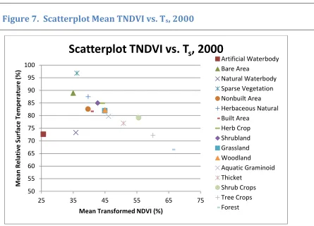
Within the Landsat 7 scenes selected for this investigation there are 16 major land cover classes each with one to nine subtypes (table 1). The most prevalent land cover types by area are: Natural Herbaceous, followed by Shrubland. Of the five natural herbaceous subtypes, closed to open herbaceous with sparse shrubs is the most common, comprising 70% of the total type area. Of the four shrubland subtypes, the most common, comprising 72% of the total type area, is very open shrubs with closed to open herbaceous and sparse trees. This corresponds to the major climate zones within the study area of Arid Steppe and Tropic Savannah. As expected, there appears to be a general inverse relationship between TNDVI and Ts (figure 7& 8). The areas which are the most vegetated have the lowest
temperatures, especially in the large forest area with a high TNDVI in the northwest corner. Comparing the means of TNDVI and Ts demonstrates this clear relationship. Outliers to the
general negative correlation demonstrated here are the natural waterbody, artificial
the lowest Ts, the lowest TNDVI type did not have the highest Ts. Artificial Waterbody,
Natural Waterbody, and Bare Area had lower TNDVI and lower Ts for both years. Bare area
includes “sand” (97.3%) and “bare soil” (2.7%) subtypes, neither of which would be expected to have any significant rooted vegetation. Neither would artificial Waterbody or Natural Waterbody be expected to have significant vegetation, except for the natural Waterbody subtype “riverbanks” (2.0%). However, excluding these three land use types, “Sparse Vegetation” has both the lowest TNDVI and highest Ts. Therefore, the artificial
Waterbody, Natural Waterbody, and bare area types will be excluded from any further discussion, figures, or charts because they cannot be expected to contain any appreciable vegetation and it is irrelevant to discuss TNDVI in these land cover types. Excluding these three types increases the Spearman’s correlation coefficient of mean TNDVI and Ts for all
50 55 60 65 70 75 80 85 90 95 100
25 35 45 55 65 75
M e an R e lativ e Su rface Tem p e ratu re (% )
Mean Transformed NDVI (%)
Scatterplot TNDVI vs. T
s, 2000
The Built-up area catagory includes the capital of Kenya, Nairobi, along with the surrounding cities of Thika, Ngong, and Machakos. It has been demonstrated that urban areas can be distinctly delineated from surrounding natural landcover by their thermal properties (Yaun and Baur, 2006; Weng et al., 2003). A strong heat island effect was not identified between Nairobi and the surrounding country side. Nairobi can be identified as green on the Ts image (figure 9 &10). It is possible this is due to the suburban, moderately vegetated
nature of the city, or perhaps a greater effect could be identified at a smaller scale. Some of the land cover types have maintained their relative positions on this graph between 2000 and 2005 (table 5). Natural and Forest, Treecrop, Thicket, Shrubcrop,
Woodland, Sparse Vegetation, Built Areas, and Natural Herbaceous are in approximately the same place relative to the others. Aquatic Graminoid, Shrubland Grassland, Herb Crop, and
50 55 60 65 70 75 80 85 90 95 100
25 35 45 55 65 75
M e an R e lativ e S u rface Te m p e ratu re (% )
Mean Transformed NDVI (%)
Scatterplot TNDVI vs. T
s, 2005
Nonbuilt areas have all changed position relative to the others. In general the first group is composed mainly of perennial and evergreen plants that do not lose their leaves or die during the dry season. The second group appears to be composed of annual and deciduous plants that lose their leaves and die back during the dry season. Although on the ground
precipitation data is not available for this study in order to corroborate such assumptions, changes in available moisture are one explanation for this variation.
The average Ts across all land cover types was 83.84% (+-7.87) (30° K or 35° C) in
2000 and 73.96% (+-8.70) (300.7° K or 27.6° C) in 2005 (figure 11). The highest average Ts
was in the Sparse Vegetation type with 96.8% (+-3.27) (319.5° K or 46.4° C) in 2000 and 84.12% (+-5.15) (309.06° K or 35.9° C) in 2005. The sparse vegetation type has only one subtype of sparse herbaceous and sparse shrubs. The lowest TOA is in the Forest type with 66.64% (+-5.8) (294° K or 21° C) in 2000 and 51.7% (+-9.3) (282.5° K or 9.4° C) in 2005.
The high average surface temperature in 2000 suggests that there is extensive
unvegetated soil and low soil moisture in the study area. It further suggests that precipitation in February 2000 was lower than average, and possibly at drought levels. Precipitation data from this area at this time are needed to support or refute this conclusion, and could not be obtained for this study. The standard deviation of the data increased from 2000 to 2005. This is possibly due to an increase in vegetation from 2000 to 2005, which would increase the variation in temperatures. Areas that contain both soil and vegetation would increase in 2005, resulting in higher variation. Direct comparison of temperatures has limited utility in this region due to major elevation change. The forest type is mainly in the mountainous
average adiabatic lapse rate is 6.4 C/km and with a total elevation change of greater than 3,000 meters across the region, this could be a significant factor when comparing land cover types. However, within land cover types this effect should be moderated due to the elevation specificity of land cover types. Furthermore, the extreme skew of the forest cover types Ts in
0 10 20 30 40 50 60 70 80 90 100 Sp ar se Ve ge ta tio n N o n b u ilt Are a H erb ace o u s N at u ra l Bu ilt Are a H erb Cr o p Sh ru b lan d G ra ss lan d Wo o d lan d Aq u at ic G ra m in o id Th icket Shru b Crop s Tre e C ro p s Fore st
Land Cover Type Random Sample (n=2000, except for nonbuilt, n=1608)
Ts Box and Whisker Chart Landsat 7 scene 168,61 February 2005
50.00 60.00 70.00 80.00 90.00 100.00 Sp ar se … N o n b u ilt Are a Bu ilt Are a H erb Cr o p Sh ru b lan d G ra ss lan d Wo o d lan d Aq u at ic… Th icket Sh ru b Cro p s Tre e C ro p s Fore st R e lativ e S u rface Te m p ar atu re (% )
Land Cover Type Random Sample (n=2000, except for nonbuilt, n=1608)
Ts Box and Whisker Chart Landsat 7 scene 168,61 February 2000
Green vegetation characteristically reflects light in the near infrared band and absorbs light in the red band, resulting in an NDVI near +1 or a TNDVI near 100%. Different
minerals found in cement, asphalt, rock, or soil tend to reflect either equal light in bands 3 and 4, or they have higher absorption in the near infrared than in the red wavelengths. In
figures 4 & 5 large tracks of vegetation can be identified, especially in the northwest and southeast corners, interspersed with large tracks of non-vegetated area. According to the land cover map (figure 6), the large vegetated tracts in the northwest and southeast are mostly forest, although in the southeast the forest is thin and surrounded by mixed land cover areas that were not included in this study (figure 12 & 13).
0 10 20 30 40 50 60 70 80 90 Sp ar se Ve ge ta tio n N o n b u ilt Are a H erb ace o u s N at u ra l Bu ilt Are a H erb Cr o p Sh ru b lan d G ra ss lan d Wo o d lan d Aq u at ic G ra m in o id Th icke t Sh ru b Cro p s Tre e C ro p s Fore st Tr an sf o rm e d N o rm al ize d Di ff e re n tial Veget ation Ind ex (% )
Land Cover Type Random Sample (n=2000, except for nonbuilt, n=1608)
TNDVI Box and Whisker Chart Landsat 7 Path 168, Row 61 February
2000 0 10 20 30 40 50 60 70 80 90 Sp ar se Ve ge ta tio n N o n b u ilt Are a Bu ilt Are a H erb Cr o p Sh ru b lan d G ra ss lan d Wo o d lan d Aq u at ic G ra m in o id Th icket Sh ru b Cro p s Tre e C ro p s Fore st
Land Cover Type Random Sample (n=2000, except for nonbuilt, n=1608)
TNDVI Box and Whisker Chart Landsat 7 Path 168,Row 61 February
2005
The Spearman’s correlation coefficient (figure 15) is a non-parametric
technique for assessing the relationship between an independent (TNDVI) and dependent (TOA) variable based on the relative ranking of each variable in a series of replications. Because the Spearman’s coefficient is approximated by the t distribution for n>100, the tcritical
is very small and all of the values are significant at alpha=0.01. The correlation between the two variables is highly dependent on the land cover type being investigated. It has been well documented that TNDVI correlates significantly with leaf area index, plant cover, and
phytomass (Sellers, 1985). Ts is a reflection of the partitioning of sensible and latent heat flux
due to evapotranspiration, which is directly related to vegetation characteristics, as well as soil water content (Owen et al., 1998). Therefore, TNDVI and Ts together may offer more
31.61 0.54 20.60 -31.89 -13.53 -32
.33 -16.50 -17.61
-31.89 -25.51 -34.25
-39.60
-23.15
-31.89 -38.16 -25.51
Art. W at er Bare Area N at . Wa te r Sp ar se Ve g. N o n b u ilt He rb ace ou s Bu ilt Are a H erb Cr o p s Sh ru b lan d G ra ss lan d Wo o d lan d Aq .G ra m . Th icket Sh ru b Cro p s Tre e C ro p s Fore st Sp e ar m an 's R an k Co rr e lation Co e ff ic ie n t
Land Cover Type Random Sample (n=2000, except for nonbuilt, n=1607)
TNDVI and Ts Correlation By Land Cover Type, 2005 (adjusted for t distribution, See Zar, 1972)
*tcritical (α=0.01, df=∞)= +/-2.327
25.81
0.00
30.24
-41.68
4.11
-36.18 -23.03 -33.32 -0.4135
91
-48.86 -52.66
-20.31
-40.94 -41.68 -43.61 -48.05
Art. W at er Bare Area N at . Wa te r Sp ar se Ve g. N o n b u ilt H erb ace o u s Bu ilt Are a H erb Cr o p s Sh ru b lan d G ra ss lan d Wo o d lan d Aq .G ra m . Th icket Sh ru b Cro p s Tre e C ro p s Fore st Sp e ar m an 's R an k Co rr e lation Co e ff ic ie n t
Land Cover Type Random Sample (n=2000, except for nonbuilt, n=1607)
TNDVI and Ts Spearman's Correlation By Land Cover Type, 2000 (adjusted for t distribution, see Zar, 1972)
*tcritical (α=0.01, df=∞)= +/-2.327
Figure 16 shows the change in ρ between 2000 and 2005 for each land cover type. These Spearman coefficient values have been scaled to correspond to a t distribution, as described in Zar (1972). According to the t distribution of α=0.01 and infinite degrees of freedom, a difference greater than or equal to 2.327 is considered significant. According to
figure 11, all land cover types had a significantly different Spearman’s correlation coefficient in 2000 from 2005, except Built-up Area, Nonbuilt area, Shrub Crops, Shrubland, and
Woodland. The correlation coefficient increased for the following types: Herbaceous, Aquatic Graminoid, and Treecrop. For the following types the correlation coefficient decreased: Forest, Grassland, Herbcrop, and Thicket. It is unclear at this time whether the change in correlation is due to land cover change, or other geophysical change.
-60 -40 -20 0
-60 -40 -20 0
ρ
2000
ρ 2005
Change in Spearman's coefficent (ρ) from 2000
to 2005
Tukey’s Honest Significant Difference (HSD) is used to identify land cover types whose average ranking of Ts or TNDVI are not significantly different, for either years (table 2 & 3). Each metric and year is assessed separately, resulting in four groups (TNDVI 2000, TNDVI 2005, Ts 2000, and Ts 2005) with 13 treatment groups each (Artificial and Natural
Waterbodies, and Bare Area are excluded), assessed at the α=0.01 level. For both TNDVI and Ts, the following groups are significantly different from all others in both 2000 and 2005
(independent): Thicket, Treecrop, Sparse Vegetation, and Forest. Types that were not significantly different in Ts in 2000 did not change in 2005. However, Herb Crop and
Woodland are the only types with TNDVI average rankings not significantly different in either 2000 or 2005. All other groups show significant change in TNDVI average ranking between 2000 and 2005. Shrubland is independent in 2000 only, and Herbaceous is independent in 2005 only. Aquatic Graminoid, Built Area, Shrubland, and Shrubcrop had significantly different TNDVI average rankings in 2000, but not in 2005. Herbaceous was not significantly different in TDNVI in 2000, but was in 2005.
Between 2000 and 2005, all types except Forest had significantly different Ts average
by deciduous or annual vegetation: Aquatic Graminoid, Grassland, Herbaceous, Herb Crop, Nonbuilt, Shrubcrop, and Thicket.
By comparing the relative average ranking of TNDVI and Ts between 2000 and 2005,
we can observe how the two metrics changed relative to one another over the course of five years. We see a dramatic difference in change in ranking between the two metrics. TNDVI relative ranking (table 5) changed between 2000 and 2005 for all land cover types except Forest and Tree Crop. In contrast, Ts relative ranking (table 6) changed between 2000 and
2005 for only grassland and woodland. This suggests that Ts is more robust than TNDVI and
less affected by inter-annual short term climate fluctuations. This makes Ts a better candidate
for land cover classification, because it is less likely to change ranking between wet and dry years. Therefore, even if absolute values change within land cover types, the difference does not change between land cover types. Furthermore, it is possible that the land cover types themselves have changed. For example, the woodland and grassland Ts relative ranking
change from 2000 to 2005 could be the process of land cover change due to natural or
Table 2. Tukey Honest Significant Difference Test (α=0.01) 2000
Landcover
Type
TNDVI Not Sign. Different
From:
Temp. Not Sign. Different
From:
Aquatic Gram.
Sbrub Crop
Built Area
Grassland, Woodland
Forest
Grassland
Herbaceous Crop, Woodland Woodland, Built Area
Herbaceous
Non-built
Herb Crops
Grassland, Woodland
Nonbuilt
Herbaceous
Shrub Land
Sparse Veg.
Shrubcrop
Aquatic Graminoid
Thicket
Treecrop
Woodland
Grassland, Herbcrop
Built Area, Grassland
Table 3. Tukey Honest Significant Difference Test (α=0.01) 2005
Landcover
Type
TNDVI Not Sign. Different
From:
Temp. Not Sign. Different
From:
Aquatic Gram.
Shrub Crop
Shrub Crop
Built Area
Grassland, Non-built
Grassland, Woodland
Forest
Grassland
Built Area, Non-built
Woodland, Built-area
Herbaceous
Herb Crop
Shrubland, Woodland
Nonbuilt
Built Area, Grassland
Shrub Land
Herb Crop
Sparse Veg.
Shrubcrop
Aquatic Gram.
Aquatic Gram.
Thicket
Treecrop
Table 4. Tukey Honest Significant Difference Test (α=0.01)
Landcover
Type
TNDVI significantly
Different from 2000 to
2005?
T
ssignificantly Different
from 2000 to 2005?
Aquatic Gram.
Yes
Yes
Built Area
No
Yes
Forest
No
No
Grassland
Yes
Yes
Herbaceous
Yes
Yes
Herb Crops
Yes
Yes
Nonbuilt
Yes
Yes
Shrub Land
No
Yes
Sparse Veg.
No
Yes
Shrubcrop
Yes
Yes
Thicket
Yes
Yes
Treecrop
No
Yes
Woodland
No
Yes
Table 5. TNDVI Relative Rank
Landcover
Type
2000
2005
Aquatic Gram.
5
4
Built Area
10
11
Forest
1
1
Grassland
6
12
Herbaceous
12
9
Herb Crops
8
7
Nonbuilt
11
10
Shrub Land
9
8
Sparse Veg.
13
3
Shrubcrop
3
13
Thicket
4
5
Treecrop
2
2
Table 6. Ts Relative Rank
Landcover
Type
2000
2005
Aquatic Gram.
9
9
Built Area
8
8
Forest
13
13
Grassland
7
6
Herbaceous
2
2
Herb Crops
3
3
Nonbuilt
5
5
Shrub Land
4
4
Sparse Veg.
1
1
Shrubcrop
10
10
Thicket
11
11
Treecrop
12
12
VI.
Discussion
Soil moisture also greatly affects Ts due to the relationship between latent and sensible
heat. Differences in soil moisture could affect the rate of evapotranspiration, and in turn the surface temperature, regardless of differences in vegetation composition and condition. This is a possible source of error in this investigation, and more work is needed to differentiate the effects of land cover and soil moisture on surface temperature. Although precipitation data was not available for the study area location, it is possible to categorically and graphically distinguish between wet and dry years. Band 5 (middle infrared) is often used to assess soil moisture levels. Because Band 5 is not affected by clay composition or vegetation types, and because water completely absorbs radiation in this band, it is useful for assessing the
moisture content of surface material. Because moisture content is indirectly proportional to reflected light in this band, areas with high moisture content will appear dark in this band, and low moisture will appear bright.
Another source of uncertainty in this investigation is the a priori land cover classification that was used for this study. Due to the possibility of land cover change between the two dates, it is difficult to ascertain with certainty whether differences in the TNDVI and Ts
relationship were due to land cover change or other geophysical change, such as climate. If this investigation were to be repeated, it would be preferable to classify the land cover in each year independently, and extrapolate the results so that land cover change would be removed as a source of variation.
One facet of this problem which this research does not address is that of time. Although measurements are taken at two points in time, each is only a single snapshot of the
electromagnetic spectrum reflected by the earth’s surface. Therefore, this research demonstrates the variability in two dimensional space of this relationship, but it does not adequately test the variability of this relationship in time. For example, these landsat 7 scenes are taken during mid-day, the period of maximum sunlight exposure. What would this same relationship demonstrate if the scenes were at night-time, during the period of minimum sunlight? I would suggest that the relationship is buffered by the presence of surface
vegetation and if this relationship were tested during the night-time the surface temperatures would be lowest in bare areas and highest in vegetated areas. Therefore, I hypothesize that non-vegetated areas have more extreme surface temperatures, higher than vegetated areas during the day-time but lower during the night-time.
scenes that was relatively uniform across all land cover types. This difference is most likely due to a difference in soil moisture due to either a late or early start to the summer rainy season, respectively. Without accurate climate data, it can only be speculated as to what is the exact factor that caused such a significant different. February is on average the hottest month in this region, and is also the end of the summer dry season. Therefore, it is likely that either the rains began early in the 2005 scene or began late in the 2000 scene.
Further research is also needed to ascertain the relationship between
evapotranspiration and energy transformation. The partitioning of waste heat as latent and sensible heat is directly related to biomass and soil moisture, which can be inferred from TNDVI and Ts. This is a fertile area of research with a huge applicability towards the
quantitative assessment of ecosystem degradation. In the past this research has been relegated to the realm of theoretical ecology and demonstrated with mathematical models only.
However, the existence of massive data sets of remote sensing imagery represents more answers than questions about the spatial and temporal variability of the behavior of electromagnetic radiation within ecosystems.
VII.
Conclusion
The main objective of this research was to evaluate the relationship between TOA temperature and TNDVI across land cover types. Based on the results of this evaluation, it can be concluded that the relationship between TOA temperature and TNDVI varies greatly across land cover types, from positive, to nil, to negative. Land cover types with complete vegetative cover exhibit the strongest correlation, and types with incomplete to no vegetative also exhibit the strongest correlation. This study agrees with conclusions of prior research, which suggest that surface cover temperature is an excellent supplementary data source for land cover classification.
However, as a data source for land cover change analysis Ts and TNDVI both performed
poorly in this study. This poor performance illustrates the sensitivity of both metrics to exogenous variables and the need for multiple data sets in any land cover classification or change study.
This study has shown that different ecosystems process solar energy differently and the correlation between temperature (Ts) and leafy green biomass (TNDVI) is generally
VIII.
References
Addiscott, T. M. (2010). Entropy, non-linearity and hierarchy in ecosystems. Geoderma, 160(1), 57-63.
Allen, Timothy FH, and Hoekstra, Thomas W. (1992).Toward a unified ecology. Columbia University Press.
Chander, G., Markham, B. L., & Helder, D. L. (2009). Summary of current radiometric calibration coefficients for Landsat MSS, TM, ETM+, and EO-1 ALI sensors. Remote sensing of environment, 113(5), 893-903.
Chavez, P. S. (1996). Image-based atmospheric corrections-revisited and improved.
Clark, R.N., Swayze, G.A., Wise, R., Livo, E., Hoefen, T., Kokaly, R., Sutley, S.J. (2007) USGS digital spectral library splib06a: U.S. Geological Survey, Digital Data Series 231.
Dash, P., Gottsche, F. -M., Olesen, F. -S., & Fischer, H. (2002). Land
surface temperature and emissivity estimation from passive sensor data: Theory and practice-current trends. International Journal of Remote Sensing, 23(13), 2563–2594.
Deering, D. W., & Rouse, J. W. (1975). Measuring'forage production' of grazing units from Landsat MSS data. In International Symposium on Remote Sensing of Environment, 10 th, Ann Arbor, Mich (pp. 1169-1178))
Ellis, J. E., and D. M. Swift. (1988). Stability of African pastoral ecosystems: alternate paradigms and implications for development. J. Range Manage. 41: 450-459. FAO (1997) Africover Land Cover Classification. FAO; Rome.
Geonetwork (2012). Spatially Aggregated Multipurpose Landcover Database for Kenya – AFRICOVER. Metadata. Retrieved July 29, 2013, from
http://www.fao.org/geonetwork/srv/en/metadata.show?currTab=simple&id=38179
Goode, P. R., & Pallé, E. (2007). Shortwave forcing of the Earth's climate: Modern and historical variations in the Sun's irradiance and the Earth's reflectance. Journal of Atmospheric and Solar-Terrestrial Physics, 69(13), 1556-1568.
Luvall, J. C., & Holbo, H. R. (1989). Measurements of short-term thermal responses of coniferous forest canopies using thermal scanner data. Remote sensing of environment, 27(1), 1-10.
Owen, T. W., Carlson, T. N., & Gillies, R. R. (1998). An assessment of satellite remotely-sensed land cover parameters in quantitatively describing the climatic effect of urbanization. International Journal of Remote Sensing, 19(9), 1663-1681.
Peel, M. C., Finlayson, B. L., & McMahon, T. A. (2007). Updated world map of the Köppen-Geiger climate classification. Hydrology and Earth System Sciences Discussions, 4(2), 439-473.
Qin, Z. H., Karnieli, A., & Berliner, P. (2001). A mono-window algorithm for retrieving land surface temperature from Landsat TM data and its application to the Israel-Egypt border region. International Journal of Remote Sensing, 22(18), 3719-3746. Schneider, E. D., & Kay, J. J. (1994). Life as a manifestation of the second law of
thermodynamics. Mathematical and computer modelling, 19(6), 25-48.
Sellers, P. J. (1985). Canopy reflectance, photosynthesis and transpiration. International Journal of Remote Sensing, 6(8), 1335-1372.
Sobrino, J. A., Jiménez-Muñoz, J. C., & Paolini, L. (2004). Land surface temperature retrieval from LANDSAT TM 5. Remote Sensing of Environment, 90(4), 434-440. Soil Survey Staff. 1999. Soil taxonomy: A basic system of soil classification for making and
interpreting soil surveys. 2nd edition. Natural Resources Conservation Service. U.S. Department of Agriculture Handbook 436.
Southworth, J. (2004). An assessment of Landsat TM band 6 thermal data for analysing land cover in tropical dry forest regions. International Journal of Remote Sensing, 25(4), 689-706.
Steinborn, W., & Svirezhev, Y. (2000). Entropy as an indicator of sustainability in agro-ecosystems: North Germany case study. Ecological Modelling, 133(3), 247-257. Transeau, E.N., 1926. The accumulation of energy by plants. Ohio J. Sci., 26: 1--10.
Toutin, T. (2004). Review article: Geometric processing of remote sensing images: models, algorithms and methods. International Journal of Remote Sensing, 25(10), 1893-1924.
Vermote, E. F., Tanré, D., Deuze, J. L., Herman, M., & Morcette, J. J. (1997). Second simulation of the satellite signal in the solar spectrum, 6S: An overview. Geoscience and Remote Sensing, IEEE Transactions on, 35(3), 675-686.
World Resources Institute. (2007). Nature’s Benefits in Kenya, An Atlas of Ecosystems and Human Well-Being. Washington, DC and Nairobi: World Resources Institute.
Ulanowicz, R. E., & Hannon, B. M. (1987). Life and the production of entropy. Proceedings of the Royal society of London. Series B. Biological sciences, 232(1267), 181-192. Ulanowicz, R. E., Goerner, S. J., Lietaer, B., & Gomez, R. (2009). Quantifying
sustainability: resilience, efficiency and the return of information theory. ecological complexity, 6(1), 27-36.
Zar, J. H. (1972). Significance testing of the Spearman rank correlation coefficient. Journal of the American Statistical Association, 67(339), 578-580.