NOTE
A Simulation Study of Permutation, Bootstrap,
and Gene Dropping for Assessing Statistical
Signi
fi
cance in the Case of Unequal Relatedness
Riyan Cheng* and Abraham A. Palmer*,†,1 *Department of Human Genetics and†Department of Psychiatry and Behavioral Neuroscience, the University of Chicago, Chicago, Illinois 60637
ABSTRACTWe used simulations to evaluate methods for assessing statistical significance in association studies. When the statistical model appropriately accounted for relatedness among individuals, unrestricted permutation tests and a few other simulation-based methods effectively controlled type I error rates; otherwise, only gene dropping controlled type I error but at the expense of statistical power.
D
ETERMINING statistical significance thresholds is an essential part of quantitative trait locus (QTL) mapping. Computationally efficient methods have been proposed to obtain significance thresholds via approximating the test statistic by an Ornstein–Uhlenbeck diffusion process (Lander and Botstein 1989; Dupuis and Siegmund 1999; Zouet al.2001) or Davis’ approximation (Davis 1987; Rebaï 1994; Piepho 2001) or by estimating the effective number of in-dependent tests (Cheverud 2001; Moskvina and Schmidt 2008). However, these methods may not provide satisfactory results (Zou et al. 2001; Dudbridge and Gusnanto 2008). Simulation-based tests are still recommended (Lander and Schork 1994) and have been used extensively in QTL map-ping. Permutation tests (Fisher 1935) have been a standard method with which to estimate significance thresholds in QTL mapping since they were introduced for this purpose by Churchill and Doerge (1994). Problems may arise when complex mapping populations or complicated statistical analyses are used (Zou et al. 2006; Churchill and Doerge 2008). In these situations, naive application of unrestricted permutation tests may lead to invalid inference because the fundamental assumption of exchangeability is violated. This problem typically occurs in mapping populations where
individuals share varying degrees of genetic relatedness and has raised questions about whether permutation tests should be applied in such situations (Abneyet al.2002; Zou
et al. 2005; Peirceet al.2008; Chenget al.2010).
In this study, we performed extensive simulations to evaluate the permutation test as well as several other simulation-based methods: parametric bootstrapping (Efron 1979), gene dropping and genome reshuffling for advanced intercross permutation (GRAIP), for assessing significance us-ing linear mixed effect models and advanced intercross lines (AIL) (Darvasi and Soller 1995), where individuals are known to be genetically unequally related. The primary purpose of this work was to investigate the performance of these meth-ods with respect to type I error rates and statistical power in the context of statistical modeling and to provide useful in-sight in the choice of methods for estimating significance thresholds when subjects are genetically unequally related. In contrast to Valdar et al.(2009), which focused on mod-eling, our study focuses on methods for determining signi-ficance thresholds when relatedness is a concern. We report our main findings while leaving the details in Supporting Information,File S1,File S2, andFile S3.
Simulation Results
We generated an AIL pedigree and sampled 576 individuals from F26 (Table S1). The phenotype was generated such
that polygenic variation approximately accounted for 56, 46, or 32% of the total phenotypic variation, corresponding to the standard deviation 0.7, 1, or 1.5 of the residual effect. Copyright © 2013 by the Genetics Society of America
doi: 10.1534/genetics.112.146332
Manuscript received October 1, 2012; accepted for publication December 6, 2012 Supporting information is available online athttp://www.genetics.org/lookup/suppl/ doi:10.1534/genetics.112.146332/-/DC1.
1Corresponding author: Department of Human Genetics, University of Chicago, 920 E. 58th St., CLSC-507D, Chicago, IL 60637. E-mail: [email protected]
Type I error
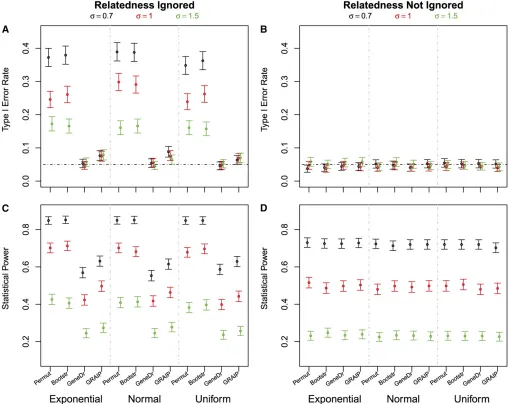
First, we ignored polygenic variation. Only the gene-dropping method effectively controlled the type I error rates; all other methods produced inflated type I error rates (Figure 1A). The larger the polygenic variation was relative to the environmen-tal variation, the more seriously the type I error rates were inflated. GRAIP performed much better than either bootstrap or permutation but was still not able to control false positives at the expected significance level.
Next we took polygenic variation into account. All the methods controlled type I error rates at the expected levels (Figure 1B). Misspecification of the residuals produced somewhat overly con-servative results, but had little impact overall (Table S2).
Statistical power
One QTL was generated with a heritability of2.8, 2.3, or 1.6%, corresponding to the standard deviation 0.7, 1, or 1.5
of the residual effect. Figure 1C reports power even when type I error is not controlled (e.g., permutation, bootstrapping). This reflects a combination of both true and false positives. The power was comparable for all of the four methods when poly-genic variation was accounted for in the model (Figure 1D). Notably, gene dropping has a higher statistical power when the relatedness was accounted for (Figure 1, C and D).
Simulations with different family sizes and subpopulation structure
We performed additional simulations by randomly choosing 288 individuals from the F26 sample and 288 individuals
from a real data set (see below). The results were similar (data not shown), suggesting that variable family size did not negatively affect the procedures. We then considered different allele (A/a) frequencies at the founder generation: 3/1 for F26vs.1/3 for F34. Under these conditions both
per-mutation and bootstrap failed to control type I error when the Figure 1 Type I error rates and statistical power. Type I error rates (A and B) and statistical power (C and D) estimated at genome-wide significance level 0.05 by each of the following methods: permuting genotypic data (Permut), bootstrapping phenotypic data (Bootstr), gene dropping (GeneDr), and GRAIP. The distribution of the residual was exponential, normal, or uniform, each with a standard deviation 0.7, 1, or 1.5.
residual was exponentially distributed and permutation also failed to control type I error when the residual was uni-formly distributed (Table 1). This is broadly consistent with our main point, which is that when the model used to ana-lyze the data are correctly chosen, permutation is an effec-tive strategy for analyzing the data.
Real data example
We used a data set from a 34th generation of a mouse AIL, which consisted of body weight measurements and geno-types for 688 mice at 3105 SNPs (Chenget al.2010; Parker
et al.2011). We did not perform the exact GRAIP procedure; instead, we shuffled simulated F33 haplotype pairs within
sex and then simulated F34genotypes. This simplified the
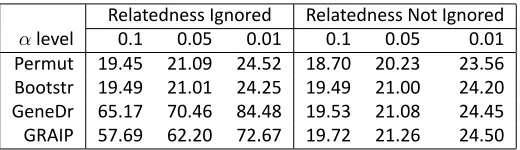
analysis while maintaining the key property of GRAIP, i.e., its ability to retain relatedness solely for full sibship. The estimated thresholds were similar when polygenic variation was accounted for in the model (Table S3). Both permuta-tion and bootstrap produced similar thresholds regardless of whether polygenic variation was ignored or accounted for in the model. In contrast, both gene dropping and GRAIP yielded significantly larger thresholds when polygenic vari-ation was ignored.
Discussion
There has been widespread concern about the use of permu-tation tests in complex mapping designs (Abney et al.2002; Zou et al. 2005; Churchill and Doerge 2008; Peirce et al.
2008). In a previous publication we observed that permuta-tion and gene dropping produced similar thresholds in the analysis of an AIL when polygenic variation was incorpo-rated in the model (Chenget al.2010); however, that article did not explore thefinding, consider alternative methods, or explore statistical power. Here we studied four simulation-based methods for obtaining empirical significance thresh-olds: permuting genotypes, bootstrapping phenotypes, gene
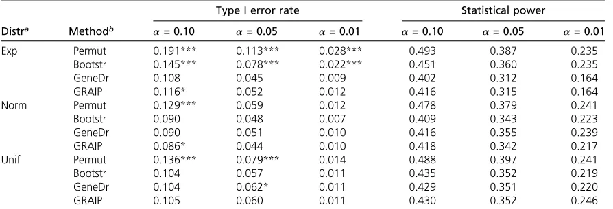
dropping, and GRAIP. The permutation test has been a stan-dard simulation-based method in QTL mapping, the boot-strap test is among the most useful empirical methods in statistics and has been recommended in mixed effect models (Pinheiro and Bates 2000; Valdar et al. 2009), and gene dropping is appropriate when pedigree information is avail-able. We found that all these methods worked well when polygenic variation was appropriately taken into account in the model; however, when polygenic variation was ignored, only gene dropping was able to control type I error rates and this came at the expense of statistical power (Figure 1, C and D). Thus, it is important to specify an appropriate statistical model in QTL mapping, especially in complex populations such as AIL; an inappropriate model can invalidate statistical inference. These principles should extend to general cases where unequal relatedness or a population structure exists. We found that the estimated distribution of the test statistic under the null hypothesis (no real QTL) was similar whether or not polygenic variation was accounted for in the model for some of the methods we examined but not for others (Table S4). In particular, the estimated distribution was significantly different when using gene dropping and GRAIP but not when using bootstrap or permutation. The take-home message is that if the model is appropriate for a genome-wide scan, we may ignore the random polygenic effect to reduce computation when performing permutation tests to estimate the significance threshold. We also found that when the polygenic variation was accounted for in the model, the estimated distributions of the test statistic for all the four methods were not significantly different from one another. One possible explanation for this is that the trait values of genetically related individuals tend to be similar and thus the test statistic is inflated because of the con-founding effect between the genotype and the phenotype adjusted for other effects in the model when the polygenic variation is ignored. Gene dropping (or to a lesser extent GRAIP) retains the relationship and is therefore capable of Table 1 Estimated Type I Error Rate and Statistical Power
Type I error rate Statistical power
Distra Methodb a= 0.10 a= 0.05 a= 0.01 a= 0.10 a= 0.05 a= 0.01
Exp Permut 0.191*** 0.113*** 0.028*** 0.493 0.387 0.235
Bootstr 0.145*** 0.078*** 0.022*** 0.451 0.360 0.235
GeneDr 0.108 0.045 0.009 0.402 0.312 0.164
GRAIP 0.116* 0.052 0.012 0.416 0.315 0.164
Norm Permut 0.129*** 0.059 0.012 0.478 0.379 0.241
Bootstr 0.090 0.048 0.007 0.409 0.343 0.223
GeneDr 0.090 0.051 0.010 0.416 0.355 0.239
GRAIP 0.086* 0.044 0.010 0.418 0.342 0.217
Unif Permut 0.136*** 0.079*** 0.014 0.488 0.397 0.241
Bootstr 0.104 0.057 0.011 0.435 0.352 0.219
GeneDr 0.104 0.062* 0.011 0.429 0.351 0.220
GRAIP 0.105 0.060 0.011 0.430 0.352 0.246
Allele (A/a) frequencies at the founder generation: 3/1 for F26vs.1/3 for F34. Estimated from 1200 simulations at genome-wide significance levela= 0.10, 0.05 or 0.01.*,**, and***indicate that the estimated type I error rate is significantly different from the expected significance levels 0.10, 0.05, and 0.01, respectively.
aResidual distribution: exponential (Exp), normal (Norm), or uniform (Unif).
bPermuting marker data (Permut), bootstrapping phenotypic data (Bootstr), or gene dropping (GeneDr).
controlling the false-positive rate regardless of the inclusion of polygenic variation. The permutation (or bootstrap) test largely dissolves the confounding and therefore provides similar thresholds regardless of whether or not the poly-genic variation is accounted for in the model, and it cannot control the false-positive rate if the polygenic variation is ignored.
Our observations were mainly based on AIL data. It is worth pointing out that the permutation test, as well as the bootstrap test, should be used with caution. Model appro-priateness such as independency, normality, and constancy of residuals is a general concern in statistical modeling. We showed that the permutation test was not robust to mis-specification of the residual distribution when the population was structured with different allele frequencies (Table 1). In addition, a major QTL (or a polygene with relatively large effects) may result in false positives due to uncontrolled confounding between the QTL (or polygene) and a scanning locus. In such a case, incorporating major QTL and possibly a few loci with relatively large effects as covariates in the model may address this concern (Valdaret al.2009; Segura
et al.2012).
Acknowledgments
We acknowledge the valuable input of Mark Abney and Andrew Skol on topics related to this work. We also appreciate the useful discussions with Gary Churchill, Karl Broman, Saunak Sen, and William Valdar. This project was supported by National Institutes of Health grants DA024845, DA021336, and MH079103.
Literature Cited
Abney, M., C. Ober, and M. S. McPeek, 2002 Quantitative-trait homozygosity and association mapping and empirical genome-wide significance in large, complex pedigrees: fasting serum-insulin level in the hutterites. Am. J. Hum. Genet. 70: 920–934. Cheng, R., J. E. Lim, K. E. Samocha, G. Sokoloff, M. Abney
et al.2010 Genome-wide association studies and the problem of relatedness among advanced intercross lines and other highly recombinant populations. Genetics 185: 1033–1044.
Cheverud, J. M., 2001 A simple correction for multiple compari-son in interval mapping genome scans. Heredity 87: 52–58. Churchill, G. A., and R. W. Doerge, 1994 Empirical threshold
values for quantitative trait mapping. Genetics 138: 963–971. Churchill, G. A., and R. W. Doerge, 2008 Naive application of
permutation testing leads to inflated type i error rates. Genetics 178: 609–610.
Darvasi, A., and M. Soller, 1995 Advanced intercross lines, an experimental population for fine genetic mapping. Genetics 141: 1199–1207.
Davis, R. B., 1987 Hypothesis testing when a nuisance parameter is present only under the alternative. Biometrika 74: 33–43. Dudbridge, F., and A. Gusnanto, 2008 Estimation of significance
thresholds for genomewide association studies. Genet. Epide-miol. 32: 227–234.
Dupuis, J., and D. Siegmund, 1999 Statistical methods for map-ping quantitative trait loci from a dense set of markers. Genetics 151: 373–386.
Efron, B., 1979 Bootstrap methods: another look at the jackknife. Ann. Stat. 7(1): 1–26.
Fisher, R. A., 1935 The Design of Experiment. Hafner Press, New York.
Lander, E. S., and D. Botstein, 1989 Mapping mendelian factors underlying quantitative traits using RFLP linkage maps. Genet-ics 121: 185–199.
Lander, E. S., and N. J. Schork, 1994 Genetic dissection of com-plex traits. Science 265: 2037–2048.
Moskvina, V., and K. M. Schmidt, 2008 On multiple-testing cor-rection in genome-wide association studies. Genet. Epidemiol. 32: 567–573.
Parker, C. C., R. Cheng, G. Sokoloff, J. E. Lim, A. D. Skol et al., 2011 Fine-mapping alleles for body weight in LG/J·SM/J F2 and F34 advanced intercross lines. Mamm. Genome 22: 563–571. Peirce, J. L., K. W. Broman, L. Lu, E. J. Chesler, G. Zhou et al., 2008 Genome reshuffling for advanced intercross permutation (GRAIP): simulation and permutation for advanced intercross population analysis. PLoS ONE 3(4): e1977.
Piepho, H.-P., 2001 A quick method for computing approximate thresholds for quantitative trait loci detection. Genetics 157: 425–432.
Pinheiro, J. C., and D. M. Bates, 2000 Mixed-Effects Models in S and S-PLUS. Springer-Verlag, New York.
Rebaï, A. B., 1994 Approximate thresholds of interval mapping tests for QTL detection. Genetics 138: 235–240.
Segura, V., B. J. Vilhjalmsson, A. Platt, A. Korte, U. Serenet al., 2012 An efficient multi-locus mixed-model approach for ge-nome-wide association studies in structured populations. Nat. Genet. 44(7): 825–830.
Valdar, W., C. C. Holmes, R. Mott, and J. Flint, 2009 Mapping in structured populations by resample model averaging. Genetics 182: 1263–1277.
Zou, F., J. A. L. Gelfond, D. C. Airey, L. Lu, K. F. Manly et al., 2005 Quantitative trait locus analysis using recombinant in-bred intercrosses: theoretical and empirical considerations. Ge-netics 170: 1299–1311.
Zou, F., B. S. Yandell, and J. P. Fine, 2001 Statistical issues in the analysis of quantitative traits in combined crosses. Genetics 158: 1339–1346.
Zou, F., Z. Zu, and T. Vision, 2006 Assessing the significance of quantitative trait loci in replicable mapping populations. Genet-ics 174: 1063–1068.
Communicating editor: G. A. Churchill
GENETICS
Supporting Information
http://www.genetics.org/lookup/suppl/doi:10.1534/genetics.112.146332/-/DC1
A Simulation Study of Permutation, Bootstrap,
and Gene Dropping for Assessing Statistical
Signi
fi
cance in the Case of Unequal Relatedness
Riyan Cheng and Abraham A. Palmer
File S1
Supplemental Material: A Simula on Study of Permuta on, Bootstrap and Gene Dropping for Assessing Sta s cal Significance
in the Case of Unequal Relatedness
This supplement contains a number of sec ons that are meant as reference material that extends on the level of detail provided
in the main text. It is not designed to be read from beginning to end and does not conform to a narra ve format in the way a journal
ar cle might.
Sta s cal Model
A typical gene c model for mapping a diploid popula on with allelesAandaat a locus is as follows
yi=xxxi0βββ+x∗ia∗+zi∗d∗+ui+i, i= 1,2,· · ·, n (1)
whereyiis the trait value for thei-th individual,xxxirepresents covariates (e.g. sex) andβββare the corresponding effects,x∗iis1,0or
−1if the genotype at the puta ve QTL isAA,Aaoraaanda∗is the addi ve effect of the puta ve QTL,zi∗is1if the genotype at the
puta ve QTL is heterozygous or0if the genotype is homozygous andd∗is the dominance effect,uirepresents polygenic varia on,
andidenotes the residual effect. Assume thati∼N(0, σ2), i= 1,2,· · ·, nare independent, anduuu= (u1, u2,· · ·, un)0 ∼
Nn(000, GGG)withGGG= (gij)and is independent of = (1, 2,· · ·, n)0. It is known (Jackquard, 1974; Abney et al., 2000) that in
general
gij = 2Φijσ2a+ ∆ij,7σd2+ (4∆ij,1+ ∆ij,3+ ∆ij,5)Cov(a, d)
+∆ij,1σh2+ (∆ij,1+ ∆ij,2−fifj)µ2h
def
= gij(a)σa2+g
(d)
ij σ
2
d+g
(ad)
ij Cov(a, d)
+gij(h)σ
2
h+g
(m)
ij µ
2
h (2)
whereΦijis the kinship coefficient between thei-th andj-th individuals,fiis the inbreeding coefficient for thei-th individual,
∆ij's are iden ty coefficients as defined in Lynch and Walsh (1998, pp.133) and can be calculated from the pedigree data, andg(ija)
denotes2Φijetc. Abney et al. (2000) suggested that the last three polygenic variance components,σ2h,Cov(a, d)andµ2h, ingij
are negligible, and we ignored these three variance components for ease of computa on. Though it is common to only consider the
addi ve polygenic variance component (e.g. Yu et al., 2006; Kang et al., 2008), we prefer to keep both the addi ve and dominance
polygenic variance components.
Permuta on, Bootstrap, Gene Dropping and Genome Reshuffling for Advanced
Intercross Permuta on
The following four simula on-based methods for es ma ng significance thresholds were used:
Permuta on testsA permuta on test is a randomiza on test. It is a re-sampling procedure. Typically, the data points are
randomly reassigned to subjects and then the permuted data is reanalyzed to obtain the test sta s c. The process is repeated
many mes. The values of the test sta s c obtained from the permuted data are treated as a sample from the distribu on of
the test sta s c of the original data under the null hypothesis, and the threshold at significance levelαis then es mated by the
100(1−α)th percen le of this set of values.
A fundamental requirement for valid permuta on is exchangeability, which should be ensured by the design of an experiment
or be assumed under the null hypothesis (Anderson, 2001; Nichols and Holmes, 2001). A permuta on test is exact when
permu-ta on is performed within exchangeable units. Exact permupermu-ta on tests do not exist when dapermu-ta points are not exchangeable, for
instance, in a linkage analysis where a con nuous variable is used as a covariate. In this case, one may consider approximate
per-muta on tests. Different strategies have been proposed to perform approximate perper-muta on tests, including perper-muta on of the
raw data or residuals under null hypothesis (see e.g. Anderson, 2001), restricted permuta on (Zou et al., 2005), and permuta on
of transformed residuals (Abney et al., 2002). The performance of approximate permuta on tests varies in different experimental
designs (Anderson and Braak, 2003).
Permu ng the phenotypic data and permu ng the genotypic data are two different ways to perform permuta on in QTL
map-ping. We permuted genotypic data, which would retain the rela onship between the trait and other predictors (e.g. sex) and could
result in be er es ma on (O'Gorman, 2005).
Bootstrap testsBootstrap is another popular re-sampling procedure. Bootstrap has a wide range of sta s cal applica ons
including hypothesis tes ng (e.g. Efron and Tibishirani, 1993). There are two versions of bootstrap: non-parametric bootstrap
and parametric bootstrap. While non-parametric bootstrap draws samples from the original data with replacement, parametric
bootstrap generates data from a fi ed model. We now briefly discuss how to use parametric bootstrap in our situa on. Under the
hypothesis of no QTL, model (1) reduces toyi=xxxi0βββ+ui+i, i= 1,2,· · ·, nandyyy= (y1, y2,· · ·, yn)0∼Nn(xxxβββ, GGG+IIIσ2)
withxxx= (xxx1, xxx2,· · ·, xxxn)0andGGG= (g
(a)
ij σ
2
a+g
(d)
ij σ
2
d). We can fit the model and obtain parameter es matesββˆβ,σˆa2,ˆσd2andˆσ2,
and then generate a sampleyyy(b)= (y1(b), y (b) 2 ,· · ·, y
(b)
n )0fromNn(xxxβββ,ˆ GGGˆ+IIIσˆ2)withGGGˆ = (g(ija)σˆ
2
a+g
(d)
ij σˆ
2
d). When polygenic
varia on is ignored,yyy(b)is generated fromNn(xxxβ, IIIββˆ σˆ2)instead. We then analyzeyyy(b)the same way as we analyze the original
datayyy. The values of the test sta s c calculated from a number (say 1000) of bootstrap samples are pooled to es mate significance
thresholds in the same way we described for permuta on tests. Our approach should be similar to what is described in ``Alterna ve
mapping methods 2'' in Valdar et al. (2009).
Gene dropping testsGene dropping is yet another re-sampling procedure. Instead of re-sampling phenotypes, it uses pedigree
informa on and Mendelian segrega on principles to generate genotypic data. The idea is straigh orward. If we know the
haplo-types in a pair of parents and recombina on rates between loci, we can simulate haplohaplo-types (and thus genohaplo-types) in an offspring
by simula ng meiosis. If we know the haplotypes in the founders, a full pedigree and a gene c map, we can simulate genotypes
for any individuals in the pedigree (see Cheng et al., 2010, for more details). Gene dropping has been used to assess significance
in a wide range of applica ons such as gene c variability (MacCluer et al., 1986; Pardo et al., 2005; Thomas, 1990), inbreeding and
allele sharing (Suwanlee et al., 2007; Jung et al., 2006), and genome-wide associa on studies (Cheng et al., 2010). A limita on of
gene dropping is the need for a pedigree.
GRAIPGenome reshuffling for advanced intercross permuta on, or GRAIP, was proposed by Peirce et al. (2008) for situa ons
where relatedness is a concern but a complete pedigree is not available. The haplotype pairs in the parents of the last genera on
are permuted across the parents within each sex and then genotypic data for the individuals in the last genera on are generated
from the permuted haplotypes by gene dropping, using the pedigree informa on about nuclear families only. As the haplotypes in
the parents are unknown in prac ce, one needs to derive phase data for the parents. This was not an issue in our studies because
the haplotype (and thus genotype) data were generated using the gene dropping procedure so phase was known.
Simula on Details
Addi onal details of our simula on studies are provided here:
Generate a pedigreeWe used advanced intercross lines (AIL) as our mapping popula on. We created a pedigree of twenty-six
genera ons from two inbred founder strains. In Fn(2 ≤n < 25), there were 144 breeding pairs and each pair produced one
female and one male progeny. The 144 female progeny randomly paired with the 144 male progeny to breed the next genera on.
Each breeding pair in F25had four progeny, which created our sample of size 576. This pedigree resulted in varying relatedness
among F26individuals (supplemental table S1 ).
Simulate genotypic and phenotypic dataIt was assumed that there were twenty chromosomes and 101 markers were evenly
distributed every 1 cM on each chromosome. One of every five markers on the second ten chromosomes were chosen as polygenic
QTL to generate polygenic varia on. The addi ve and dominance effects of the polygenic QTL were randomly uniformly distributed
in(−0.2,0.2)and(−0.04,0.04)respec vely.
Phenotypic data were generated from equa on (1), with an overall mean0and polygenic effects as stated above. The
related-ness measurements were calculated from the pedigree as described in Cheng et al. (2010). The standard devia onσof the residual
iwas0.7,1or1.5, and the corresponding polygenic effects on average approximately accounted for 56%, 46%, or 32% of the total
varia on in the phenotype. Genotypic data were generated by gene dropping using the pedigree.
To inves gate robustness of a test to misspecifica on of the residual's distribu on, we generated data from exponen al and
uniform distribu ons in addi on to normal distribu ons.
Obtaining significance thresholdsWe used four methods to test for QTL: permuta on, parametric bootstrap (e.g. Efron and
Tibishirani, 1993), gene dropping and genome reshuffling for advanced intercross permuta on (GRAIP) Peirce et al. (2008). In
the permuta on test, we permuted genotypic data without restric on unless specified otherwise. We were especially interested
to inves gate the performance of the permuta on test in the context of sta s cal modeling. In applica ons, one may choose
restricted permuta on if appropriate.
Type I errorThe genome scan for QTL under the null hypothesis of no QTL was performed on the first ten chromosomes, where
there were no QTL. For each set of parameter values, 1200 datasets were generated and each dataset was analyzed using the
likelihood ra o test (LRT). The type I error rate was es mated by the propor on of the 1200 datasets for which one or more of
the scanned markers were iden fied as QTL, meaning that the test sta s c exceeded the genome-wide significance threshold at
a given significance level. We generated 6000 datasets to es mate significance thresholds for each of the four methods and each
set of parameter values.
The data were analyzed with polygenic varia on either being ignored or being accounted for. If polygenic varia on was ignored,
the model to analyze the data wasyi=µ+x∗ia∗+zi∗d∗+i, i= 1,2,· · ·, n; this was model (1) without the random polygenic
effect.
Sta s cal powerIn new sets of simula ons, a QTL was placed in the middle of the first chromosome. The QTL had an addi ve
effect 0.4 and a dominance effect 0.1. The QTL accounted for approximately 2.8%, 2.3%, or 1.6% of the total variance,
correspond-ing toσ = 0.7,1or1.5. Again, the genome scan for QTL under the null hypothesis of no QTL was performed on the first ten
chromosomes. A QTL was iden fied if the test sta s c at any of the scanning loci exceeded the genome-wide threshold at a given
significance level. For each of the four methods and each set of parameter values, the power was es mated by the propor on of
1200 simula ons where a QTL was iden fied. The threshold was es mated in the same way as for type I error rates.
Pooling Procedure
In prac ce when we have one dataset, we can permute the dataN mes to es mate a threshold for the test sta s c. When we
replicate a simula onK mes, the test sta s c in all the replicates follows the same distribu on. Therefore, we only need one
threshold for all the replicates. Suppose we permute the dataNi mes in thei-th replicate simula on and getSi ={xij, j =
1,2,· · ·, Ni},i= 1,2,· · ·, K. Then
E{
∑K i=1
∑Ni j=1Ixij>x
∑K i=1Ni
}=
∑K i=1αNi
∑K i=1Ni
=α
wherexis the100(1−α)th percen le ofSiandIxij>x = 1ifxij > xor0otherwise. This means that we can poolSi(i=
1,2,· · ·, K)to es mate the threshold for the test sta s c in all the replicate simula ons.
Computa onal Approxima on
In general there is no analy cal solu on to maximum likelihood es mates (MLE) for model (1). Genome scans are extremely
computa onally intensive and some mes imprac cal without computa onal simplifica on. Note that the random effectuin model
(1) is only used to control background gene c varia on. A reasonable approxima on will be good enough. Assume in equa on
(2)gij(a)σ
2
a+g
(d)
ij σ
2
d+g
(ad)
ij Cov(a, d) +g
(h)
ij σ
2
h+g
(m)
ij µ
2
h = (g
(a)
ij c1 +gij(d)c2+g(ijad)c3+g(ijh)c4+g(ijm)c5)σ
2. Then the
variance-covariance matrix ofyyyisΣΣΣ = (GGG(a)c
1+GGG(d)c2+GGG(ad)c3+GGG(h)c4+GGG(m)c5+III)σ2whereGGG(a)= (g (a)
ij )etc. Ifc's
are known, then 1
σ2ΣΣΣis a known matrix and an analy cal MLE solu on exists. In applica ons,c's are unknown; however, we can
es mate them under the null hypothesis and use the es mates as known values. Approxima ng random effects by their es mates
is a known strategy in mixed-effect model models (Pinheiro and Bates, 2000) and works well in our situa on.
Computa onal Efficiency
The permuta on test as well as the other three methods is computa onally intensive, which is a trade-off between reliability and
computa on. However, the computa on is s ll manageable with the previous computa onal approxima on even if there are
thousands of markers. In our simula ons, there were 1010 SNP markers and the sample size was 576; one genome scan took only
a few seconds on a conven onal desktop computer. Parallel compu ng can make it realis c to perform permuta on tests even
when there are hundreds of thousands of SNP markers.
References
Abney, M., M. S. McPeek, and C. Ober (2000). Es ma on of variance components of quan ta ve traits in inbred popula ons.Am.
J. Hum. Genet. 141, 629--650.
Abney, M., C. Ober, and M. S. McPeek (2002). Quan ta ve-trait homozygosity and associa on mapping and empirical genome-wide
significance in large, complex pedigrees: fas ng serum-insulin level in the hu erites.Am. J. Hum. Genet. 70, 920--934.
Anderson, M. J. (2001). Permuta on tests for univariate or mul variate analysis of variance and regression. Can. J. Fish. Aquat.
Sci. 58, 626--639.
Anderson, M. J. and C. J. F. T. Braak (2003). Permuta on tests for mul -factorial analysis of variance. J. Stat. Comput. Simul. 73,
85--113.
Cheng, R., J. E. Lim, K. E. Samocha, G. Sokoloff, M. Abney, A. D. Skol, and A. A. Palmer (2010). Genome-wide associa on studies
and the problem of relatedness among advanced intercross lines and other highly recombinant popula ons. Gene cs 185,
1033--1044.
Efron, B. and R. Tibishirani (1993).An introduc on to the bootstrap. Chpman & Hall, Inc.
Jackquard, A. (1974).The gene cs structure of popula ons. Springer-Verlag, NY.
Jung, J., D. E. Weeks, and E. Feingold (2006). Gene-dropping vs. empirical variance es ma on for allele-sharing linkage sta s cs.
Genet. Epidem. 30, 652--665.
Kang, H. M., N. A. Zaitlen, C. M. Wade, A. Kirby, D. Heckerman, M. J. Daly, and E. Eskin (2008). Efficient control of popula on
structure in model organism associa on mapping.Gene cs 178, 1709--1723.
Lynch, M. and B. Walsh (1998).Gene cs and analysis of quan ta ve traits, Volume 5. Sinauer Associates, Inc.
MacCluer, J. W., J. L. VandeBerg, B. Read, and O. A. Ryder (1986). Pedigree analysis by computer simula on.Zoo Biology 5, 147--160.
Nichols, T. E. and A. P. Holmes (2001). Nonparametric permuta on tests for func onal neuroimaging: a primer with examples.
Human Brain Mapping 15, 1--25.
O'Gorman, T. W. (2005). The performance of randomiza on tests that use permuta ons of independent variables.Commun. Stat.
Sim. Comput. 34, 895--908.
Pardo, L. M., I. MacKay, B. Oostra, C. M. van Duijin, and Y. S. Aulchenko (2005). The effect of gene c dri in a young gene cally
isolated popula on.Ann. Hum. Genet. 69, 288--295.
Peirce, J. L., , K. W. Broman, L. Lu, E. J. Chesler, G. Zhou, D. C. Airey, A. E. Birmingham, and R. W. Williams (2008). Genome reshuffling
for advanced intercross permuta on (GRAIP): simula on and permuta on for advanced intercross popula on analysis. PLoS
ONE 3(4), e1977.
Pinheiro, J. C. and D. M. Bates (2000).Mixed-effects models in S and S-PLUS. Springer-Verlag, New York.
Suwanlee, S., R. Baumung, J. S¨lkner, and I. Curik (2007). Evalua on of ancestral inbreeding coefficients: Ballou's formula versus
gene dropping.Conserv. Genet. 8, 489--495.
Thomas, A. (1990). Comparison of an exact and a simula on method for calcula ng gene ex nc on probabili es in pedigrees.Zoo
Biology 9, 259--274.
Valdar, W., C. C. Holmes, R. Mo , and J. Flint (2009). Mapping in structured popula ons by resample model averaging.Gene cs 182,
1263--1277.
Yu, J., G. Pressoir, W. H. Briggs, I. V. Bi, M. Yamasaki, J. F. Doebley, M. D. McMullen, B. S. Gaut, D. M. Nielsen, J. B. Holland, S. Kresovich,
and E. S. Buckler (2006). A unified mixed-model method for associa on mapping that accounts for mul ple levels of relatedness.
Nat. Genet. 38, 203--208.
Zou, F., J. A. L. Gelfond, D. C. Airey, L. Lu, K. F. Manly, R. W. Williams, and D. W. Threadgill (2005). Quan ta ve trait locus analysis
using recombinant inbred intercrosses: theore cal and empirical considera ons.Gene cs 170, 1299--1311.
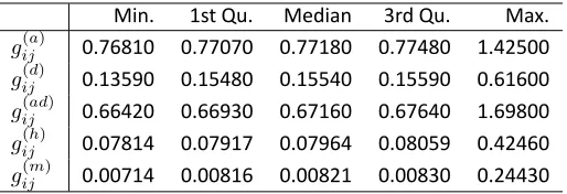
Table S1 Summary of Relatednessa
Min. 1st Qu. Median 3rd Qu. Max.
gij(a) 0.76810 0.77070 0.77180 0.77480 1.42500
gij(d) 0.13590 0.15480 0.15540 0.15590 0.61600
gij(ad) 0.66420 0.66930 0.67160 0.67640 1.69800
gij(h) 0.07814 0.07917 0.07964 0.08059 0.42460
gij(m) 0.00714 0.00816 0.00821 0.00830 0.24430 a Defined in equa on (2) among the simulated F
26individuals. The different levels of relatedness means that the assump on of exchangeability is incorrect.
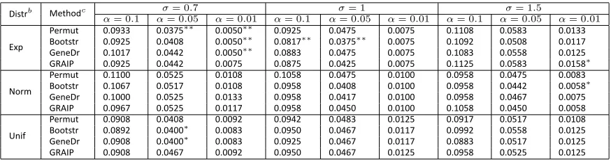
Table S2 Type I Error Ratesa
Distrb Methodc σ= 0.7 σ= 1 σ= 1.5
α= 0.1 α= 0.05 α= 0.01 α= 0.1 α= 0.05 α= 0.01 α= 0.1 α= 0.05 α= 0.01
Exp
Permut 0.0933 0.0375∗∗ 0.0050∗∗ 0.0925 0.0475 0.0075 0.1108 0.0583 0.0133 Bootstr 0.0925 0.0408 0.0050∗∗ 0.0817∗∗ 0.0375∗∗ 0.0075 0.1092 0.0508 0.0117 GeneDr 0.1017 0.0442 0.0050∗∗ 0.0883 0.0475 0.0075 0.1083 0.0558 0.0125 GRAIP 0.0925 0.0442 0.0075 0.0875 0.0425 0.0075 0.1125 0.0583 0.0158∗
Norm
Permut 0.1100 0.0525 0.0108 0.1058 0.0475 0.0100 0.0958 0.0475 0.0083 Bootstr 0.1067 0.0517 0.0108 0.0958 0.0408 0.0100 0.0958 0.0442 0.0058∗ GeneDr 0.1000 0.0525 0.0133 0.0958 0.0417 0.0100 0.0958 0.0467 0.0075 GRAIP 0.0967 0.0525 0.0117 0.0958 0.0450 0.0100 0.1058 0.0450 0.0058
Unif
Permut 0.0908 0.0408 0.0092 0.0942 0.0483 0.0125 0.0917 0.0517 0.0108 Bootstr 0.0892 0.0400∗ 0.0083 0.0950 0.0467 0.0117 0.0992 0.0558 0.0125 GeneDr 0.0908 0.0400∗ 0.0083 0.0925 0.0467 0.0117 0.0883 0.0517 0.0125 GRAIP 0.0908 0.0467 0.0092 0.0950 0.0467 0.0125 0.0958 0.0525 0.0125
aEs mated from 1200 simula ons at genome-wide significance levelsα=0.10, 0.05 and 0.01. Symbol∗,∗∗or∗∗∗indicates the
es mated type I error rate is significantly different from the expected level at significance level 0.10, 0.05 or 0.01.
bPermu ng genotypic data (Permut), bootstrapping phenotypic data (Bootstr), gene dropping (GeneDr) or GRAIP.
cThe distribu on of the residual was exponen al (Exp), normal (Norm) or uniform (Unif), each with a standard devia on
0.7,1or 1.5.
Table S3 Es mated Genome-wide Thresholds for the Body Weight Data
Relatedness Ignored Relatedness Not Ignored
αlevel 0.1 0.05 0.01 0.1 0.05 0.01
Permut 19.45 21.09 24.52 18.70 20.23 23.56
Bootstr 19.49 21.01 24.25 19.49 21.00 24.20
GeneDr 65.17 70.46 84.48 19.53 21.08 24.45
GRAIP 57.69 62.20 72.67 19.72 21.26 24.50
Es mated from 5000 simula ons at genome-wide significance levelsα=0.1, 0.05 and 0.01 by the following methods: permu ng genotypic data (Permut), bootstrapping phenotypic data (Bootstr), gene dropping (GeneDr) and GRAIP, using the likelihood ra o test (LRT).
Table S4 P-values by the Kolmogorov-Smirnov Test
Permut Bootstr GeneDr GRAIP
σ= 0.7 0.60200 0.32428 0.00000 0.00000
σ= 1 0.44558 0.44988 0.00000 0.00000
σ= 1.5 0.43282 0.10871 0.00000 0.00000
Based on 6000 simula ons under the null hypothesis that when no QTL effects existed, the distribu on es mated by a tes ng method when relatedness was ignored was iden cal to the distribu on es mated by the same method when relatedness was taken into account. Data was generated by each of the tes ng methods: permu ng genotypic data (Permut), bootstrapping phenotypic data (Bootstr), gene dropping (GeneDr) and GRAIP. The distribu on of the residual was normal with a standard devia on0.7,1or1.5.
R. Cheng and A. A. Palmer 11 SI
Supporting Data and R Scripts
Available for download at http://www.genetics.org/lookup/suppl/doi:10.1534/genetics.112.146332/-‐/DC1.